Abstract
Introduction. A new algorithm that uses a grid-based technique to solve the linear Boltzmann transport equation (LBTE) has been developed to improve the accuracy and speed of external photon beam treatment planning calculations. The aim of this study was to test the accuracy of this algorithm in both heterogeneous and homogeneous media. Material and methods. Output factors, depth dose curves and profiles for symmetric fields were measured in water using diamond and ionization chamber detectors. Furthermore, asymmetric fields, fields collimated with the multi-leaf collimator, enhanced dynamic wedge fields as well as fields with different source-skin distances were measured. Various test plans were created on a CIRS thorax phantom including tissue-equivalent inserts and corresponding dose distributions within the phantom were measured with radiochromic films. The new grid-based LBTE solver, Acuros XB (Eclipse version 10.0, Varian Medical Systems, CA, USA) was used to calculate dose distributions for all field configurations and plans, for both 6 MV and 15 MV photons. Calculations were also performed with AAA, a standard convolution algorithm. Results. Compared to measurements, the output factors were within 1% for Acuros XB. For the depth doses, the average deviations were within 1% in dose and 1 mm in distance to agreement (DTA). For the profiles, the deviations were within 2%/1 mm except near the penumbra. Similar results were obtained for the other field configurations. Good agreement with AAA was also found. For the plans calculated on the CIRS phantom, the number of points meeting the gamma criterion of 3% in dose and 3 mm in DTA was higher with Acuros XB (98% for 6 MV; 100% for 15 MV) than with AAA (94% for 6 MV; 96% for 15 MV). Conclusion. Dose calculations with the Acuros XB algorithm in homogeneous media are in good agreement with both measurements and the AAA algorithm. In heterogeneous media, the Acuros XB algorithm is superior to AAA in both lung and bony material.
In order to optimize the outcome of radiotherapy (RT), the development of more precise planning and delivery methods is a constantly ongoing process. The International Commission on Radiation Units has recommended an overall accuracy of maximum 5% in the delivery of absorbed dose [Citation1] and the American Association of Physicists in Medicine has recommended that the uncertainty in the computed dose distribution is less than 2% [Citation2]. These constraints on the dose distribution may be fulfilled for most present dose calculation algorithms when considering homogeneous tissue. However, simple pencil beam algorithms fail in calculating the dose to heterogeneous media, due to a very simplified modelling of electron transport. Large deviations may be observed in the lung tissue [Citation3–10] and to a minor extent in bony structures [Citation5,Citation6,Citation8,Citation11], as the electron density of these tissues deviates substantially from water. A more precise calculation of the absorbed dose is obtained by advanced convolution algorithms [Citation4–10]. These algorithms use pre-calculated Monte Carlo (MC) dose kernels, which are scaled locally to approximate the electron transport in the presence of heterogeneities. Numerous studies have tested and compared different types of calculation algorithms [Citation2,Citation11–13] and deviations above 2% in heterogeneous tissue have been found even for these advanced algorithms. In these studies, the algorithms have been validated against dosimetric measurements in phantoms or against MC calculations. In the ideal situation of an infinite number of particles and correct particle interaction data, the MC dose calculation will be equal to the absorbed dose in the medium. However, MC calculation is rather time consuming and therefore not used routinely for dose calculation. In contemporary RT, rather complex treatment techniques, such as volumetric modulated arc therapy (VMAT), may introduce long dose calculation times which are problematic in particular in the setting of adaptive image-guided RT.
A new algorithm, Acuros XB, which explicitly solves the linear Boltzmann transport equation (LBTE) has recently been introduced into the Eclipse treatment planning system (TPS) (Varian Medical Systems, CA, USA) [Citation16,Citation17]. The LBTE is a set of two coupled equations describing the transport and interactions of directly and indirectly ionizing particles as they travel through matter. The electron angular fluence is obtained by solving the LBTE and from this the dose may be calculated by use of the macroscopic electron energy deposition cross sections and the density of the materials. The effect of heterogeneities is therefore directly accounted for; however, knowledge of the elemental composition of the material is required.
Algorithms based on solving the LBTE differs fundamentally in heterogeneous media from pencil beam or convolution algorithms including lateral scatter which use density based corrections to approximate the dose contribution originating from changes in primary electron transport. Therefore, these algorithms are expected to reproduce the dose distributions in heterogeneous media as, e.g. lung and bony tissue more correctly than the convolution algorithms. In homogeneous media, no improvements of the algorithms based on solving the LBTE are expected compared to the convolution algorithms as both types of algorithms use MC simulations of the treatment head to obtain the photon and electron fluence in the accelerator.
In the ideal situation, i.e. without approximations, MC and explicit LBTE method solutions will converge as both algorithms are based on solving the LBTE. However, both types of algorithms require the introduction of approximations in order to be solvable. The LBTE may be solved explicitly by discretizing the variables in space, angle and energy and then iteratively solving the problem [Citation18]. Algorithms which deterministically solve the LBTE by discretizing the variables are referred to as grid-based Boltzmann solvers (GBBS). The discretization of the variables in space, angle and energy results in systematic errors dependent on the number of discrete parameters. The MC calculation method stochastically predicts particle transport through the medium by tracking the histories of random particle interactions. The errors introduced in MC calculation are random and result from simulating a finite number of particles. Furthermore, the accuracy of both types of algorithms depends on the accuracy of the cross sections used.
A dosimetric validation of the GBBS algorithm for square open and wedged fields in water has recently been reported by Fogliata et al. [Citation19]. They found the overall degree of accuracy to be within 1% for open beams when comparing to both measurements and the current standard algorithm. Furthermore, the GBBS algorithm has been tested against the BEAMnrc/DOSXYZnrc MC code using one anterior field at a heterogeneous slab phantom encompassing soft tissue, lung and bone material and agreement within 2% was found. For a computed tomography (CT) data set of a patient with tumor mass in the right lung, the agreement was found to be within 2% in dose or 2 mm in DTA [Citation20].
The aim of this study was to experimentally and comprehensively examine the accuracy of the GBBS algorithm in both homogeneous and heterogeneous phantom geometries. The accuracy of the algorithm was tested in a range of clinical situations including variable SSD, asymmetric fields, as well as for intensity modulated radiation therapy (IMRT) and VMAT treatment plans. The performance of the algorithm was compared to ionization chamber, diamond detector and film measurements as well as relative to calculations with the current standard algorithm.
Material and methods
As input to the Acuros XB implementation in the Eclipse TPS., the algorithm requires the macroscopic atomic cross sections of the components of the material [Citation16,Citation17]. Therefore, a conversion from Hounsfield units to mass density is implemented by a user-defined calibration curve. From the derived mass density, the algorithm determines the material composition from the voxels in the image by use of a predefined material library [Citation16]. The library specifies the material composition for five biological materials (lung, adipose tissue, muscle, cartilage and bone) and 16 non-biological materials. The mass density calibration curve was obtained from the scanner-specific electron density curves by use of the conversion values measured by Constantinou et al. [Citation21].
The Acuros XB algorithm supports calculation of both dose to medium, Dm and dose to water, Dw. The implementation of the algorithm consists of two parts: the photon beam source model, which is also used by the AAA algorithm, and the radiation transport model where the dose in the medium, Dm is calculated from the electron fluence obtained by the GBBS algorithm. Dm may be converted to Dw by use of the stopping power ratios between medium and water [Citation22]. Only minor differences between Acuros XB and AAA are expected in homogeneous media. The two types of algorithms may differ substantially in heterogeneous media notably different from water as, e.g. lung or dense bony tissue; Acuros XB explicitly models the physical interactions of radiation and matter whereas AAA use pre-calculated MC kernels scaled according to local density variations.
Equipment and beam data
The measurements required to configure the algorithm were performed at a Varian 2100 C/D linear accelerator, delivering 6 MV and 15 MV photon beams (Varian Medical Systems). The Eclipse TPS (version 10.0.28; Varian Medical Systems) was used in this study for both the Acuros XB and the AAA algorithm. The configuration of the Acuros XB algorithm was identical to the AAA algorithm and the same set of beam data was used. The width of the penumbra may be modelled in Acuros XB, by manually optimizing the effective spot size. A value of 1 mm was suggested by the vendor, and this was found to be optimal in the present study.
Output factors, depth dose curves, and beam profiles were measured for open fields at field sizes (FS) 1 × 1 cm2 to 40 × 40 cm2. The output factors were measured for 196 square and rectangular fields at SSD = 95 cm. Depth dose curves and profiles were measured for 14 square fields (1 × 1 cm2, 2 × 2 cm2, 3 × 3 cm2, 4 × 4 cm2, 6 × 6 cm2, 8 × 8 cm2, 10 × 10 cm2, 12 × 12 cm2, 15 × 15 cm2, 20 × 20 cm2, 25 × 25 cm2, 30 × 30 cm2, 35 × 35 cm2 and 40 × 40 cm2) at source surface distance (SSD) equal to 100 cm. The profiles were measured at five different depths d: dmax, 5 cm, 10 cm, 20 cm and 30 cm. All beam data were measured in a PTW water phantom (PTW, Freiburg, Germany). A diamond detector (PTW) was used for field sizes below 15 × 15 cm2 and a RK ionization chamber (Scanditronix–Wellhöfer, Sweden) was used for the larger field sizes. The depth dose curves, profiles and output factors measured with the diamond detector was corrected for dose rate dependencies [Citation8]. The accelerator was calibrated to 1 Gy at d = 5 cm and SSD = 95 cm for field size 10 × 10 cm2 for both energies. This is denoted the reference situation.
Homogeneous media
The algorithm was validated in a homogeneous medium for both 6 MV and 15 MV photons. Measurements were performed in the water phantom and calculations were performed in a 40 × 40 × 40 cm3 phantom with the Hounsfield units set to zero for all points. The grid size used for the calculation was 2 mm. Calculations were performed using both algorithms. Output factors, depth dose curves and profiles were investigated for a number of different beam configurations as described in the following.
The central axis (CAX) output factors used for the implementation of the algorithms were measured for square and rectangular fields for FS 1 × 1 cm2 to 40 × 40 cm2 at SSD = 100 cm and d = 5 cm. These output factors were compared to the calculated values. The dependence of SSD was investigated by analyzing CAX output factors measured at d = 5 cm at SSD = 80 cm and SSD = 130 cm for FS 4 × 4 cm2, 10 × 10 cm2 and 30 × 30 cm2. To investigate the accuracy of the algorithm for asymmetric field shapes, measurements were performed for eight asymmetric fields. The fields were created as half beams or by overtravel of either X or Y jaw or both. The output factors were measured centrally in the asymmetric field at d = 10 cm and SSD = 90 which is a clinically relevant depth. In addition, fields defined by the MLC were tested for two field sizes. A 4 × 4 cm2 field with the jaws retracted to 6 × 6 cm2 and a 10 × 10 cm2 field with the jaws retracted to 12 × 12 cm2. Output factors at CAX were measured at d = 10 cm and SSD = 90 cm. Finally, output factors at CAX were investigated at d = 10 cm and SSD = 90 cm for a 20 × 20 cm2 field with EDW of angle 30° and 60°. All output factors were normalized to the reference situation and the relative difference Dcalc/Dmeas between measured and calculated values was derived.
To investigate the dose distribution as a function of depth in the phantom, depth dose curves were measured and calculated in the water phantom. The depth dose curves at CAX were evaluated for square fields of FS 1 × 1 cm2 to 40 × 40 cm2 at SSD = 100 cm. Furthermore, depth dose curves were evaluated at SSD = 80 cm and SSD = 130 cm for FS 4 × 4 cm2, 10 × 10 cm2 and 30 × 30 cm2. In a setup at SSD = 90 cm, depth dose curves were measured and calculated centrally in eight asymmetric fields being identical to those used for output factor determination. The depth dose curves were normalized to dmax and the dose difference Dcalc – Dmeas at 10 cm and 20 cm was calculated. For the depth dose curves at SSD = 100 cm, the mean values and standard deviations (SD) for all 14 field sizes were calculated. In the region from the surface to the depth of maximum dose, the DTA was evaluated for the Acuros XB algorithm.
The dose distribution laterally in the phantom was investigated by measurement and calculation of profiles for several different field geometries. Profiles were evaluated at three depths (dmax, 10 cm, 30 cm) for the 14 field sizes measured at SSD = 100 cm used for the implementation of the algorithm. In addition, profiles were analyzed at d = 10 cm for SSD = 80 cm and SSD = 130 cm. The profiles were measured in the transversal direction, which is the direction used for the data implemented in the TPS. For the asymmetric fields described previously, profiles were measured at d = 10 cm and SSD = 90 cm. Finally, profiles were measured at d = 10 cm and SSD = 90 cm in solid water (Gammex, WI, USA) with the two dimensional (2D) ionization chamber array seven29 (PTW) for a 20 × 20 cm2 field with EDW of angle 30° and 60°. All profiles were normalized to 100% at CAX except for the asymmetric fields which were normalized to 100% centrally in the field. The relative dose difference Dcalc/Dmeas in the flattened region was calculated. The penumbra region was evaluated for profiles at d = dmax, 10 and 30 cm and SSD = 100 cm for all field sizes. The DTA in the penumbra region was calculated at 20%, 50% and 80% of the maximum dose.
Heterogeneous media
The dose distributions in heterogeneous media were measured in a CIRS Model 002LFC IMRT Thorax Phantom (CIRS, VA, USA) using Gafchromic EBT dosimetry films (ISP, NJ, USA). This phantom mimics the thoracic region of a lung cancer patient, with water, fat, muscle (ρ = 1.04 g/cm3), bone (ρ = 1.60 g/cm3) and lung (ρ = 0.21 g/cm3) tissues [Citation24].
We tested 11 different treatment plans in the CIRS phantom at both photon energies. The phantom offers the possibility to insert films for 2D dose measurements at transversal slices. The dose distribution was measured in the isocentric plane. A short description of the treatment plans is given in . Field sizes generally varied between 10 × 10 cm2 and 20 × 20 cm2, except one treatment plan with field size of 2 × 2 cm2. Some fields where shaped according to a fictive tumor and MLCs were inserted. The table angle was zero for all fields, i.e. only co-planar fields were investigated. The isocenter was located centrally in the phantom at the mediastinum except for the treatment plan with the 2 × 2 cm2 field size. In this plan, simulating small field irradiation of a spinal tumor, the isocenter was located in the spine.
Table I. Nomenclature and description of the treatment plans. For the volumetric modulated arc therapy plans the monitor units have been set to 200 MUs and 400 MUs.
All measurements were compared with the Eclipse calculations for both the Acuros XB and the AAA algorithm. Dose to water, Dw, was reported for both algorithms as the detectors were calibrated to measure Dw and this is the dose quoted for most commercial treatment planning systems. MC and GBBS based algorithms are based on Dm, which may be converted by the TPS to Dw by calculating the dose received by a very small volume of water inside the medium. This volume should be so small that it does not disturb the electron fluence. However, the measurements performed in the present work, made use of a small water-like detector (radiochromic films) that is much larger than the very small water volume used by the Acuros XB algorithm for the conversion to Dw. In order to imitate this situation, the calculations should be performed with a small water-like detector inserted at the measurement position. This relates to all non-water materials; however, significant differences should be observed for materials with stopping power ratios differing considerably from water [Citation22]. In the CIRS phantom, this only applies to the bony material component, which simulates the vertebral body. Thus in the present study, a point dose centrally at the vertebral body, Dcalculated was calculated with a 0.03 cm3 volume of water located at that position for all treatment plans. These point dose calculations were compared to the doses measured at the same point, Dfilm. The deviation was given as (Dfilm – Dcalculated)/Dfilm*100. For the Acuros XB algorithm, we also evaluated Dm. In order to test the perturbation of the film on the measurement, the dose to 10 randomly selected points in the lung phantom, was calculated by insertion of a 0.03 cm3 volume of water at these points.
All treatment plans tested in the CIRS phantom were calculated with the same number of Monitor Units (MU), for both algorithms. The dose to the isocenter was 2 Gy per fractions for all treatment plans when using the Acuros XB algorithm. As the algorithms differ, this resulted in a dose slightly different from 2 Gy for AAA.
The calibration of the Gafchromic EBT dosimetry films was performed with four separate films irradiated with known doses from 0.3 Gy to 3 Gy in a 10 × 10 cm2 field. The films were mounted parallel to the beam axis between two slabs of box shaped 30 × 30 cm2 solid water (Gammex), each of 10 cm thickness. Irradiation in this position gave rise to depth dose curves and the calibration curve was determined from a comparison of points on these curves to the similar points determined in a water phantom. The uncertainty for the Gafchromic EBT dosimetry films was approximately 2% depending on the handling of the films [Citation23,Citation24]. In reality, the “point” doses from the film calibration measurements were average doses over a small volume.
Finally, to check the accuracy and reliability of the film measurements we used a Farmer Type chamber (FC65-G, Scanditronix Wellhöfer, Germany) to measure point doses at the isocenter of the phantom (water equivalent tissue) for all the treatment plans, except the plan ‘Spine stereotactic body radiation therapy (SBRT)’.
The 2D dose distributions were evaluated in VeriSoft version 4.1 (PTW) with a Gamma criterion [Citation12] of 3% in dose (reference dose 2 Gy) and 3 mm in DTA. The number of points fulfilling this Gamma criterion was evaluated for all 22 treatment plans and the mean value and one SD was calculated for each calculation algorithm. Doses below 5% of the maximum dose were neglected. All points located at the bony structure were neglected as the film, being a water-like medium, disturbs the dose distribution, as explained previously. The size of the films was 25 × 20 cm2, which covered most or all of the irradiated area. In the following, the mean value, x, and its standard deviation (SD), y, is denoted as x ± y.
Results
Homogeneous media
Output factors for square and rectangular fields at d = 5 cm and SSD = 100 cm were compared for all field sizes. The maximum deviations were within 0.5% for both energies and algorithms, except for AAA at field sizes below 4 × 4 cm2, were a maximum deviation of 2.1% was found for field size 1 × 1 cm2 at 15 MV. Output factors measured at SSD = 80 cm and SSD = 130 cm deviated less than 1% for both energies and algorithms. Similarly, for the asymmetric fields and fields defined by the MLC, the maximum deviation of the output factors for both energies was below 0.5% for Acuros XB and below 0.7% for AAA. Finally, the output factors at CAX for EDW fields deviated by at most 0.5% from the measurements.
The depth dose curves for FS 10 × 10 cm2 and 40 × 40 cm2 are shown in . For the Acuros XB algorithm, the mean deviation and the SD for 6 MV photons was 0 ± 0.3% at d = 10 and d = 20 cm. For 15 MV photons, the mean and SD was 0.2 ± 0.2% at d = 10 cm and d = 20 cm. For the AAA algorithm, the deviations were in the range 0 ± 0.2% for both energies. For 6 and 15 MV photons, the DTA was below 1 mm for both algorithms. Depth dose curves measured at different SSDs and for asymmetric fields showed similar agreement to the measurements.
Figure 1. Depth dose curve for 6 MV and 15 MV photon beam at FS 10 × 10 cm2 and 40 × 40 cm2.
A comparison of calculated and measured profiles for FS 1 × 1 cm2, 10 × 10 cm2, 20 × 20 cm2 and 40 × 40 cm2 are shown in for 6 MV photons. For both energies the mean deviation in the flattened region was below 1% except near the penumbra region where a maximum deviation of 2% was observed (). In the penumbra region, a discrepancy above 1 mm in DTA was observed for field sizes larger than 10 × 10 cm2. The largest deviation was seen at 20% of the dose, with a maximum deviation of 6 mm or 3% for a 20 × 20 cm2 field at d = 30 cm for 6 MV photons (). For 15 MV the largest deviation was 2 mm. In general, Acuros XB underestimated the dose in the low dose region just outside the jaws. On the contrary, in the high dose region close to the penumbra, Acuros XB overestimated the dose (). These deviations were far more evident for 6 MV photons than for 15 MV photons. The AAA algorithm showed similar but less pronounced deviations. For field sizes less than 8 × 8 cm2, both algorithms overestimated the width of the penumbra but the deviations were less than 1 mm. Comparison of measured and calculated profiles at SSD = 80 cm and SSD = 130 cm showed deviations of the same order of magnitude as those measured at SSD = 100 cm. A profile measured at d = 10 cm for a 20 × 10 cm (X × Y) half beam field with 6 MV photons is shown in . DTA up to 5 mm and 2% dose deviations were seen close to the CAX. Apart from this, all deviations were comparable to those for symmetric fields. For the EDW beams, a maximum absolute deviation of 1.5% was observed.
Figure 2. A comparison of measured and calculated profiles using both Acuros XB and AAA at d = 1.5 cm, 10 cm and 300 cm for 6 MV photons. Only half of the (symmetric) profiles are shown. FS: 1 × 1 cm2, 10 × 10 cm2, 20 × 20 cm2 and 40 × 40 cm2.
Figure 3. Measured and calculated (Acuros XB and AAA) profiles for the asymmetric half beam field 20 × 10 (Y1 = −20, Y2 = 0) at d = 10 cm and SSD = 90 cm.
Heterogeneous media
The Gamma criterion was fulfilled for at least 95% of the evaluated points in all treatment plans when evaluating the measured dose distributions by the Acuros XB algorithm (see ). A similar degree of agreement was found in 15 of the 22 treatment plans when calculated with AAA. In most cases, the Gamma criterion was fulfilled for more points by the Acuros XB algorithm than by AAA. The percentage of points fulfilling the Gamma criterion was 98.2 ± 1.1% and 99.5 ± 0.3% for the Acuros XB algorithm, for 6 MV and 15 MV photons, respectively. For AAA, 94.1 ± 7.0% and 96.1 ± 3.3% of the evaluated points fulfilled the criterion for 6 MV and 15 MV photons, respectively ().
Table II. Percentage of points fulfilling the Gamma (3,3) agreement index for the treatment plans delivered with 6 MV and 15 MV photons. The mean value and standard deviation has been calculated for each energy. The treatment plans are specified in Table I.
Both algorithms overestimated the dose to part of the lung by up to 5% for Acuros XB and up to 8% for AAA in some of the treatment plans. This tendency was predominantly seen for the AAA algorithm. For the Acuros algorithm, deviations exceeding 3% were seen for small volumes only. For 15 MV, only very small deviations were seen when using Acuros XB. In addition to the overestimation in lung, the AAA algorithm also overestimated the dose close to the vertebral body, by up to 8% in some of the treatment plans. The film was found to change the dose distribution in the lung by a maximum increase of dose of 1%, typically less; this effect was neglected.
The dose centrally in the vertebral body was estimated for all 22 treatments plans from the film measurements and compared to the dose calculated in a small volume of water at the same position for both algorithms, see . For the Acuros XB algorithm, a mean deviation of 1.0 ± 1.9% and −0.1 ± 1.9% was found for 6 MV and 15 MV photons, respectively. For the AAA algorithm, a mean deviation of 2.1 ± 1.9% and 5.0 ± 1.8% was found for 6 MV and 15 MV, respectively. Only minor difference was found for the AAA algorithm when calculating dose to the vertebral body with or without insertion of a small volume of water at the calculation point.
Figure 4. Comparison of the dose measured at the films at a point centrally in the vertebral body for all 22 treatment plans, to the dose calculated at the same point for the two algorithms. The deviation in dose is given as (Dfilm – Dcalculated)/Dfilm*100. The plan number is specified in .

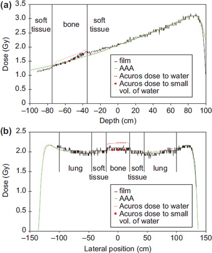
A comparison between the film measurements and the two algorithms is shown in for two selected one dimensional (1D) profiles of two of the treatment plans. shows the depth dose curve centrally at the AP field. The calculation of Dw is shown for both algorithms in addition to a point dose calculation in the bony material in seven points with the insertion of a small water detector (only shown for Acuros XB). A good agreement is seen for both algorithms. However, the AAA algorithm is seen to overestimate the dose after passing the vertebral body. In , a vertical profile at the depth of the center of the vertebral body is shown. The calculation of Dw is shown for both algorithms in addition to a point dose calculation in the bony material in three points with the insertion of a small water detector. Very good agreement is seen for both algorithms. The Dw calculation in the bony material using Acuros XB can not be compared to the measurement using film.
Figure 5. a) Depth dose curves evaluated at the central axis of the thorax phantom for the field “AP” delivered with 6 MV photons. b) Lateral profile for the field “Lat op” delivered with 6 MV photons. The profile is evaluated at the depth of the vertebral body. The calculation of dose to a small volume of water in the vertebral body was performed for Acuros XB for a few points for both fields.
For all treatment plans Dm was evaluated for the Acuros XB algorithm. Results identical to the results for Dw were found, except in the vertebral body. Centrally in this structure, the ratio of Dw to Dm was 14 ± 0.5%.
Finally, for all point dose verification measurements (Farmer chamber vs. films), agreement within 1.2% was found.
Discussion
In this study we have performed an extensive investigation of the performance of a new grid-based Boltzmann equation solver for treatment planning calculations in both homogeneous and heterogeneous geometries. In homogeneous media, output factors, depth dose curves and profiles were investigated for a variety of geometries, and the performance of the algorithm was comparable to the current standard algorithm, AAA. In heterogeneous media, deviations below 3% and 3 mm were observed for the majority of the irradiated point for all treatment plans.
The output factors were reproduced very well with deviations below 0.3% for SSD = 100 cm. The tests performed at two clinically extreme setup distances (SSD of 80 cm and 130 cm) showed similar agreement to the measured data, proving an overall good agreement to the measured data. In addition, the calculation of highly asymmetric fields and fields with an MLC or EDW showed dose deviations below 0.5% at the central point. All measurements of output factors were performed at d = 5 cm or 10 cm at which depth many tumors are located. These findings are confirming those of Fogliata et al. who reported a mean deviation of output factors calculated at d = 10 cm and SSD = 90 cm of 0.4 ± 0.2% and 0.3 ± 0.2% for 6 MV and 15 MV, respectively [Citation19]. Furthermore, the deviations observed with Acuros XB are comparable to those found for AAA.
For the depth dose curves, Acuros XB showed deviations below 1% and 1 mm. Again, this is in agreement to the findings of Fogliata et al. [Citation19]. In their results a maximum deviation of 1% in dose was observed, while 97% of the points in the build up region showed deviations of maximum 1 mm.
We found profiles to be well modelled in Acuros XB, except close to the penumbra region where the dose was overestimated in the high dose region and underestimated in the low dose region. This made the width of the penumbra too small. This effect was only observed for large field sizes. The Acuros XB algorithm will therefore underestimate the dose to an organ at risk outside but very close to the penumbra region. At larger distances (approximately 2 cm) from the field edge, the dose in the penumbra region was well modelled. These findings are again in agreement with those of Fogliata et al. [Citation19] where deviations up to 4% and 2% for 6 MV and 15 MV photons, respectively where observed outside the field for large field sizes. However, in the central beam region average dose differences below 1% was observed in accordance with the present study. For AAA slightly better agreement was found, in concordance with previous reports [Citation9,Citation26]. Profiles measured for asymmetric fields and EDW fields showed deviations below 5 mm in DTA and 2% in dose, which is comparable to the findings found for the AAA in both the present and several previous studies [Citation8,Citation9,Citation26].
For heterogeneous media, the Acuros XB calculations showed a good correspondence with measurements for both 6 MV and 15 MV photons. Overall, the Acuros XB algorithm is superior to the AAA algorithm in heterogeneous media as seen from the higher values of the Gamma agreement index. Generally, the results in lung, soft tissue and bone for the Acuros XB algorithm fulfilled the gamma criterion and the agreement was better than for the AAA algorithm.
The effect of heterogeneities on the dose distribution has been studied in several publications for pencil beam algorithms, convolution algorithms including lateral scatter as well as MC algorithms [Citation3–13,Citation18,Citation19,Citation29]. In most reports, the dose distribution in lung tissue has received most attention, as large deviations were observed between the pencil beam based algorithms and the more advanced convolution algorithms. However, only minor deviations exist between the convolution based algorithms and the MC based algorithms. Comparison to experimental data typically shows deviations below 5% for commercial convolution algorithms in normal lung tissue [Citation4–9]. In the present study, the GBBS algorithm Acuros XB showed good agreement (mostly within 3%) to the measurement in lung tissue with overestimation of the dose to lung (maximum 5%) in only a very small proportion of the calculated points, and the algorithm also performed better than the superposition algorithm, AAA. These findings for Acuros XB are in agreement with the findings of Bush et al. [Citation20], who compared Acuros XB to a MC based algorithm and found deviations below 2% in lung material. The deviations found in the present study are slightly larger, as the calculations are compared to measurements using Gafchromic films with an estimated uncertainty of 2%.
For bony structures, minor dose differences have usually been observed between the pencil beam algorithms, convolution algorithms and MC algorithms [Citation5,Citation6,Citation8,Citation11,Citation12,Citation29]. In general, pencil beam algorithms underestimate the dose to bony structures for high energy photons as these algorithms account for the increased attenuation in dense media only, without considering the increased electron fluence in the media [Citation8,Citation11]. Better agreement is found for low energy photons. In the present study, good agreement was found between the measured and calculated dose to the vertebral body for the Acuros XB algorithm. These findings are in accordance with previous work of Siebert et al. [Citation22]. Larger deviations were found for AAA especially at 15 MV, where the algorithm was found to underestimate the dose by as much as 5%. The findings for the AAA algorithm were in agreement with findings in previous studies [Citation6,Citation8,Citation9,Citation29].
When reporting dose to bony structures, there is a huge difference between reporting dose to water and dose to medium (here bone). The difference in absorbed dose between tissue and water is determined by the mass stopping power of bone and tissue which is in the order of 11%, nearly independent of energy for clinical beams [Citation22]. In the present study, the difference between calculation of dose to water and dose to bone centrally in the vertebral body was 14% ± 0.5%. This is slightly more than the value expected from the mass stopping power ratios. For soft tissue and lung tissue, a maximum difference in stopping power ratios of 1% has been found [Citation22] and thus, minor differences are expected for these tissues in agreement to the findings in the present study.
Comparing the dose in bony structures as calculated by Acuros XB and AAA gives rise to a difference of up to 15% when dose to water Dw, is evaluated (see ). Thus, a large difference in the calculated dose to the vertebral body may be observed when changing the algorithm used in the TPS from AAA to Acuros XB when keeping with the Dw evaluation. However, it should be pointed out that for calculations of dose to the spine where the spinal cord is usually the most critical organ at risk, the dose calculated by the two algorithms in the cord will be nearly identical as it is a soft tissue.
The applied CIRS thorax phantom simulates the thoracic region of the human body. The vertebral body has a diameter of 4 cm and the electron density is 1.6 g/cm3. The phantom is made of epoxy resins [Citation24] with an elemental composition fairly close to that used for bony structures by the Acuros XB algorithm. It should be pointed out that only bony structures of this elemental composition have been tested in the present study. Larger dose deviations may be observed for denser bone as only one elemental composition is used for bone.
In conclusion, this study has shown that dose calculations with the Acuros XB algorithm in homogeneous media are in good agreement with both measurements and AAA. In heterogeneous media, the Acuros XB algorithm clearly outperforms AAA, in both lung and bony material.
References
- International Commission on Radiation Units and Measurements (ICRU). Determination of absorbed dose in a patient irradiated by beams of X or gamma rays in radiotherapy procedures. ICRU Report 24. Washington, DC: ICRU; 1976. p. 67.
- American Association of Physicists in Medicine (AAPM). Tissue inhomogeneity corrections for megavoltage photon beams. Radiotherapy Committee Task Group 65, Report No. 85. Report of AAPM. Madison, WI: Medical Physics Publishing; 2004.
- Engelsman M, Damen EMF, Koken PW, van't Veld AA, van Ingen KM, Mijnheer BJ. Impact of simple tissue inhomogeniety correction algorithms on conformal radiotherapy of lung tumours. Radiother Oncol 2001;60:299–309.
- Jones AO, Das IJ. Comparison of inhomogeneity correction algorithms in small photon fields. Med Phys 2005;32: 766–76.
- Nisbet A, Beange I, Vollmar H-S, Irvine C, Morgan A, Thwaites DI. Dosimetric verification of a commercial collapsed cone algorithm in simulated clinical situations. Radiat Oncol 2004;73:79–88.
- Breitman K, Rathee S, Newcomb C, Murray B, Robinson D, Field C, . Experimental validation of the Eclipse AAA algorithm. J Appl Clin Med Phys 2007;8:76–92.
- Aspradakis MM, Morrison RH, Richmond ND, Steele A. Experimental verification of convolution/superposition photon dose calculations for radiotherapy treatment planning. Phys Med Biol 2003;48:2873–93.
- Rønde HS, Hoffmann L. Validation of Varian's AAA algorithm with focus on lung treatments. Acta Oncol 2009;48: 209–15.
- Van Esch A, Tillikainen L, Pyykkonen J, Tenhunen M, Helminen H, Siljamäki S, . Testing of the analytical anisotropic algorithm for photon dose calculation. Med Phys 2006;33:4130–48.
- Aarup LR, Nahum AE, Zacharatou C, Juhler-Nøttrup T, Knöös T, Nyström H, . The effect of different lung densities on the accuracy of various radiotherapy dose calculation methods: Implications for tumour coverage. Radiother Oncol 2009;91:405–14.
- Carrasco P, Jornet N, Duch MA, Panettieri V, Weber L, Eudaldo T, . Comparison of dose calculation algorithms in slab phantoms with cortical bone equivalent heterogeneities. Med Phys 2007;34:332–3.
- Knöös T, Wieslander E, Cozzi L, Brink C, Fogliata A, Albers D, . Comparison of dose calculation algorithms for treatment planning in external photon beam therapy for clinical situations. Phys Med Biol 2006;51:5785–807.
- Fogliata A, Vanetti E, Albers D, Brink C, Clivio A, Knöös T, . On the dosimetric behaviour of photon dose calculation algorithms in the presence of simple geometric heterogeneities: Comparison with Monte Carlo calculations. Phys Med Biol 2007;52:1363–85.
- Vestergaard A, Søndergaard J, Petersen JB, Høyer M, Muren LP. A comparison of three different adaptive strategies in image-guided radiotherapy of bladder cancer. Acta Oncol 2010;49:1069–76.
- Knap MK, Hoffmann L, Nordsmark M, Verstergaard A. Daily cone-beam computed tomography used to determine tumour shrinkage and localisation in lung cancer patients. Acta Oncol 2010;49:1077–84.
- Eclipse Algorithms Reference Guide. Palo Alto: Varian Medical Systems; 2010.
- Faille GA, Wareing T, Archambault Y, Thompson S. Acuros XB advanced dose calculation for the Eclipse treatment planning system. Palo Alto: Varian Medical Systems; 2010.
- Vassiliev ON, Wareing AW, McGhee J, Failla G, Salehpour MR, Mourtada F. Validation of a new grid-based Boltzmann equation solver for dose calculation in radiotherapy with photon beams. Phys Med Biol 2010;55:581–98.
- Faille GA, Wareing T, Archambault Y, Thompson S. Acuros XB XB advanced dose calculation for the Eclipse treatment planning system. Palo Alto: Varian Medical Systems; 2010;56:1879–904.
- Bush K, Gagne IM, Zavgorodni S, Ansbacher W, Beckham W. Dosimetric validation of Acuros XB with Monte Carlo methods for photon dose calculations. Med Phys 2011;38:2208–21.
- Constantinou C, Harrington JC. An electron density calibration phantom for CT-based treatment planning computers. Med Phys 1992;19:325–7.
- Siebers JV, Keall PJ, Nahum AE, Mohan R. Converting absorbed dose to medium to absorbed dose to water for Monte Carlo based photon beam dose calculations. Phys Med Biol 2000;45:983–95.
- Fowler JF. Solid state electrical conductivity dosimeters. In: Attix FH, Roesch WC, editors. Radiation dosimetry. New York: Academic Press; 1966.
- CIRS Inc. CIRS Tissue simulation & phantom technology [online]. Virginia: 2011. Available from: www.cirsinc.com/002lfc_rad.html [accessed 2011].
- Lynch BD, Kozelka J, Ranade MK, Li JG, Simon WE, Dempsey JF. Important considerations for radiochromic film dosimetry with flatbed CCD scanners and EBT Gafchromic® Film. Med Phys 2006;33:4551–6.
- Paelinck L, De Neve W, De Wagter C. Precautions and strategies in using a commercial flatbed scanner for radiochromic film dosimetry. Phys Med Biol 2007;52:231–42.
- Low DA, Dempsey JF. Evaluation of the gamma dose distribution comparison method. Med Phys 2003;30: 2455–64.
- Fogliata A, Nicolini G, Vanetti E, Clivio A, Cozzi L. Dosimetric validation of the anisotropic analytical algorithm for photon dose calculation: Fundamental characterization in water. Phys Med Biol 2006;51:1421–38.
- Bragg CM, Conway J. Dosimetric verification of the anisotropic analytical algorithm for radiotherapy treatment planning. Radiother Oncol 2006;81:315–23.