Modeling neuroendocrine stress reactivity in salivary cortisol: adjusting for peak latency variability

Abstract

In this report, we present growth curve modeling (GCM) with landmark registration as an alternative statistical approach for the analysis of time series cortisol data. This approach addresses an often-ignored but critical source of variability in salivary cortisol analyses: individual and group differences in the time latency of post-stress peak concentrations. It allows for the simultaneous examination of cortisol changes before and after the peak while controlling for timing differences, and thus provides additional information that can help elucidate group differences in the underlying biological processes (e.g. intensity of response, regulatory capacity). We tested whether GCM with landmark registration is more sensitive than traditional statistical approaches (e.g. repeated measures ANOVA – rANOVA) in identifying sex differences in salivary cortisol responses to a psychosocial stressor (Trier Social Stress Test –TSST) in healthy adults (mean age 23). We used plasma ACTH measures as our “standard” and show that the new approach confirms in salivary cortisol the ACTH finding that males had longer peak latencies, higher post-stress peaks but a more intense post-peak decline. This finding would have been missed if only saliva cortisol was available and only more traditional analytic methods were used. This new approach may provide neuroendocrine researchers with a highly sensitive complementary tool to examine the dynamics of the cortisol response in a way that reduces risk of false negative findings when blood samples are not feasible.

• ACTH
• growth curve modeling
• HPA
• salivary cortisol
• sex differences

Introduction

Due to the known limitations of measuring neuroendocrine stress reactivity via blood samples (Kirschbaum & Hellhammer, 1989), research with salivary cortisol has exploded during the last decades, greatly contributing to our understanding of HPA-axis functioning in a wide range of health conditions and developmental processes (Clements, 2013; Hellhammer et al., 2009). Yet, this research has been frustratingly inconsistent, which has led to calls to improve and standardize salivary cortisol methods and analytic approaches (Clements, 2013). In this report, we hope to advance these efforts by presenting Growth Curve Modeling (GCM) with landmark registration as a new statistical approach that addresses an often-ignored but important source of variability in salivary cortisol analysis: Individual and group differences in the time latency of post-stress peak concentrations (Lopez-Duran et al., 2009). Peak latency differences may obscure important findings in some contexts and common analytic approaches do not address this issue. We propose landmark registration, a non-parametric approach that involves the adjustment of individual post-stress curves upon a salient landmark (post-stress peaks), as a complementary tool in the analysis of neuroendocrine stress reactivity.

Commonly used methods to model post-stress salivary cortisol vary greatly, both in the type of information they provide and their limitations. Examination of time series data (means) via repeated measures ANOVA (rANOVA) allows researchers to compare mean differences in cortisol levels at and between specific times and as they fluctuate over time (Gueorguieva & Krystal, 2004). However, rANOVA has multiple limitations, including high vulnerability to missing data and assumption of homogeneity of covariance, which is often violated in biological samples and can result in biases in F-test calculations (Gueorguieva & Krystal, 2004; Hruschka et al., 2005; Matthews et al., 1990). Two alternatives to rANOVA have been proposed. Examination of area under the curve (AUC) via various approaches (e.g. ANOVA, OLS regression) solves some of these problems and facilitates comparisons and predictions of total cortisol output after stress (Matthews et al., 1990; Pruessner et al., 2003). Unfortunately, this approach can mask potentially meaningful differences in patterns of post-stress cortisol changes (Pruessner et al., 2003). Alternatively, time series means can be examined via random-effects models (Gueorguieva & Krystal, 2004) and specifically, multi-level growth curve modeling (Schlotz et al., 2011), which can provide more detailed characterizations of cortisol changes without the limitations of rANOVA, and therefore has been recommended for the analysis of biological repeated measures data (Gueorguieva & Krystal, 2004).

However, individuals and groups can vary in the timing of post-stress cortisol fluctuations (Lopez-Duran et al., 2009), which is not fully captured by these approaches. Although such variability may be meaningful, it complicates interpretation of simple time series, peak and AUC measures, since standard approaches cannot easily tease apart contributing components, such as rate of rise, absolute magnitude of peak, duration of rise and rate of decline, each of which may reflect different aspects of system regulation. This problem is less troublesome in studies that collect blood samples, as these allow analysis of both ACTH and cortisol levels. Since ACTH triggers the cortisol responses captured, but rises and falls with a much more rapid time course (Kumsta et al., 2007), having access to both hormones can shed more light on both the magnitude of stress reactivity and its temporal dynamics. In contrast, saliva cortisol is a number of steps removed from the brain processes of interest, with “extra” variables such as adrenal sensitivity, binding globulin levels, movement into saliva and the size of the salivary “space” all potentially altering both the size and timing of cortisol response to ACTH release (Hellhammer et al., 2009). Saliva measures, however, are more widely used and more readily accessible, so they could benefit from efforts to optimize their value through additional analytic techniques that could better differentiate system activation, response magnitudes and regulation dynamics, and perhaps thus better reflect information that may be more readily available from ACTH and cortisol measures in blood.

A known challenge with response curve data is that it is subjected to both amplitude and phase variability (Vantini & Vatini, 2012). Individuals and groups can vary in the magnitude (amplitude) of their cortisol response to stress, but also in the temporal dynamics (phase) of that response (Hellhammer et al., 2009; Lopez-Duran et al., 2009). Although these two types of variability are often intertwined and may be impacted by common factors (e.g. inhibitory feedback can impact the magnitude of response – peak – as well as the timing of the peak), these components may be shaped by different regulatory phenomena. For example, baseline levels, secretory capacity and intensity and speed of both activation and regulation can all contribute to amplitude variability (Kudielka et al., 2009), reflected in the magnitude of peak levels. In contrast, phase variability (i.e. variation in the timing or latency of slopes and peaks) may be shaped by other factors, such as the timing of adrenal activation; a complex interaction between threshold, speed and intensity of inhibitory feedback control (De Kloet, 2004); and individual differences in reactivity to various contextual aspects of stress paradigms, such as what aspect of the task individuals consider stressful (Lopez-Duran et al., 2009).

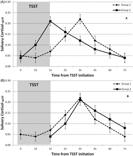
Regardless of source, timing differences can impact the assessment and interpretation of indices of amplitude variability. For example, comparisons made at specific times (e.g. 25 or 45 min) may not reflect differences in key indices of interest (e.g. reactivity or regulation) because cortisol levels at specific times can reflect different phases within each individual’s or group’s post-stress curves. For example, Figure 1(A) presents two responses to the TSST reflecting significant phase variability (timing) but limited amplitude variability. Repeated measures analysis would identify group differences at 15 and 35 min that are potentially misleading and difficult to interpret because these differences are primarily due to timing effects. Likewise, growth curve modeling from a common baseline (i.e. time 0) would suggest flatter initial slope in group 2, which implies a less reactive response. Yet, the group differences appear to be in the timing of the initiation of the activation. Additional analyses of the data presented in Figure 1(B), in which the timing differences have been removed, would be necessary to correctly test for amplitude effects. Such analyses would correctly show that the groups only vary in the timing but not the shape of their activation curve. Phase effects may have different biological meaning than the amplitude effects, but comparisons of unadjusted time series means via standard approaches (e.g. rANOVA) do not fully separate the two and do not readily capture the full range of information potentially available about both amplitude and phase variability.

Figure 1. (A) Presents two responses to the TSST reflecting significant phase variability (timing) but limited amplitude variability. The observed differences at 15 min and 35 min are likely due primarily to differences in the timing of the response. (B) Shows the same data after adjusting the curves to control for timing differences. Analysis of Figure 1(B) data would correctly show that the groups do not differ in reactivity or regulation once timing differences are accounted for.

The problem of phase/timing effects is not unique to neuroendocrine data. It is well-known in the measurement of neural signals, including ERP (Wang et al., 2001) and fMRI (Bellgowan et al., 2003), and when measuring human growth (Gasser et al., 1990). Although a number of solutions have been proposed (Jansen & Huang, 1985; Lindquist et al., 2009; Wang et al., 2001), one common approach is to align response curves on the time axis to reduce, although not fully eliminate, phase variability and allow a more precise focus on amplitude effects (Gasser et al., 1990; Kneip & Gasser, 1992; Ramsay & Li, 1998). When alignment is based on a specific feature of the curve, such as a response peak, the process is called landmark registration (Kneip & Gasser, 1992). Our approach to landmark registration of cortisol curves involves identification of individual peaks and alignment of response curves so that the estimated peaks for all individuals coincide on a fixed time point (Figure 1B). This procedure allows us to conduct a GCM to simultaneously examine individual and group differences in key features of stress reactivity, such as the peak amplitude, as well as aspects of the response curve that are often not specifically and directly examined, such as the slope to peak (reflecting potentially important aspects of activation), and the slope after peak (which may reflect important aspects of regulation), while controlling for differences in the timing of these features, which may not be relevant to some questions of interest.

In this study, we tested whether GCM with landmark registration is more sensitive than traditional approaches (i.e. rANOVA of time series means, examinations of area under the curve, traditional growth curve modeling from baseline or after recentering the time variable to the mean group peak time) to identify group differences in salivary cortisol. To this end, we examined sex differences in post-stress plasma ACTH and saliva cortisol after the Trier Social Stress Test (TSST; Kirschbaum et al., 1993). Men consistently have greater ACTH responses to psychosocial stressors compared to women (Kirschbaum et al., 1999; Kudielka et al., 2004; Kumsta et al., 2007; Uhart et al., 2006), but data on salivary cortisol is more equivocal. Three studies examined sex differences in ACTH and salivary cortisol responses to stressors (Kirschbaum et al., 1999; Kudielka et al., 2004; Kumsta et al., 2007); with two failing to find differences in cortisol despite clear differences in ACTH (Kirschbaum et al., 1999; Kudielka et al., 2004). Some studies that only assessed salivary responses reported greater responses in men (Childs et al., 2010; Kirschbaum et al., 1995; Kirschbaum et al., 1996; Kirschbaum et al., 1992; Schoofs & Wolf, 2011), but others found no sex differences (Rohleder et al., 2001; Schlotz et al., 2011). The data imply that the relationship between salivary cortisol stress response and sex may be less robust (compared to ACTH) and/or may be more sensitive to the impact of methodological and statistical artifacts, such as sex differences in peak latency that may obscure differences in reactivity (e.g., activation slope, peak levels) when traditional approaches are used. Therefore, we hypothesize that our proposed statistical approach will be more sensitive to detect underlying sex differences in salivary cortisol in response to the TSST than traditional analyses, as evidenced by providing stronger effects sizes and characterizations of sex differences that more closely resembles those found in ACTH.

Methods

Participants

The study included 54 healthy adults (21 females, 33 males, M_age = 23.41, SD_age = 6.06, age range = 18–44) who were participating in a study investigating the impact of brief cognitive interventions on HPA axis response to the TSST. They were recruited through multi-media community advertising (e.g. newspapers, internet). Interested participants were telephone screened by a trained research assistant and those meeting entry criteria were invited to a face-to-face evaluation, where they were further assessed for eligibility, using a variety of self-report measures and a structured clinical interview for DSM-IV (SCID). Qualifying participants were 18–45 years old, medically healthy, within 30% of ideal body weight, and had no recent exposure to psychoactive medication (two months), no history of substance dependence or recent abuse (six months), low levels of tobacco use (<20 cigarettes/d) and alcohol use (<8 drinks/wk), negative urine drug screen results, and normal screening laboratory results (CBC to screen for anemia). They also had no psychiatric disorders as evaluated by the SCID and no first-degree family history of anxiety (except specific phobia) or affective disorders. Female participants were premenopausal, not pregnant or lactating, not using birth control pills, and studied between days 18 and 27 of the menstrual cycle (luteal phase). Qualifying participants signed written, Institutional Review Board-approved consent, and were paid $100 for their participation. One participant was excluded due to highly atypical ACTH values suggesting invalid data. The final sample with ACTH data included 53 participants. Salivary cortisol was available from 42 participants (22 males, 20 females M_age = 23.31 23.41, SD_age = 5.96, age range = 18–43) and collected in the laboratory at the time of each blood sample, except for one sample, which was taken during speech preparation instead of after the speech task.

Procedures

The study was conducted at an academic medical research center. Intravenous access was established not later than 1:30 p.m., using an 18–20 gauge angiocatheter in an antecubital vein, kept open with a normal saline drip. Participants then rested comfortably for one hour, to allow them to accommodate to the research setting and IV. Baseline blood samples were drawn at 2:10 and 2:25 p.m. (20 min and immediately prior to stress protocol initiation). The 2:10 sample was not used in our analyses since it represented a pre-task control. After collection of the 2:25 p.m. sample, participants moved to a second room for the start of the TSST at 2:30 p.m. Additional blood samples were obtained at the end of the speech task (10 min after start), at the end of the math task (15 min after start) and at 25, 35, 45, 60 and 75 min after stress initiation (back in the accommodation room). Saliva samples were collected using cotton salivettes at the time of each blood sample, except during the TSST when saliva samples were taken at the end of speech preparation (as opposed to end of speech task) as well as at the end of the math task.

The TSST has been described extensively elsewhere (Kirschbaum et al., 1993). We followed standard procedures except for experimental variations in task instructions utilized for a parent study. Specifically, participants were randomly assigned to one of four different instruction sets upon arrival in the laboratory: Standard TSST instructions (SI) or one of three cognitive interventions that (1) provided access to control over threat exposure (by giving participants permission to close a curtain between them and the panelists to avoid social scrutiny), (2) increased familiarity and effective coping (by reassuring that emotional and physical responses were normal and expectable responses in this social challenge task and providing cognitive coping tools to make the experience feel less threatening, unexpected or unusual; see Abelson et al. (2008) for the coping intervention used in a pharmacological activation paradigm), or (3) shifted goal orientation from self-promotion to helping others (by talking about ways to use the job to contribute to a larger mission beyond their own accomplishments and promote a greater good, emphasizing other-focused or compassionate values (Burson et al., 2012). Intervention (Abelson et al., 2004) effects are being reported elsewhere. Since participants were randomized to these interventions, and sex distribution did not differ by intervention group, χ² (3, N = 54) = 1.13, p = 0.77, we did not examine or control for intervention in these analyses.

ACTH and saliva cortisol assay and processing

Assays

Cortisol was assayed using Coat-a-Count cortisol kits (Siemens, Princeton, NJ), a widely used and well-validated radioimmunoassay (RIA) with an analytical sensitivity of 0.2 mcg/dl and with an inter-assay and intra-assay variabilities of less than 5%. ACTH was assayed using a chemiluminscent assay (Immulite 1000 ACTH, Siemens, Princeton, NJ), with an analytical sensitivity of 9 pg/mL and with an inter-assay and intra-assay variabilities of less than 5%.

Salivary cortisol transformation

Saliva cortisol was transformed using Box–Cox power transformation for time series using the solution identified by Miller & Plessow (2012). Specifically, each cortisol value was transformed using the formula X′ = (X²⁶− 1)/0.26. This transformation was selected over the more traditional log transformation because it produces superior results in normalizing the distribution of cortisol scores (Miller & Plessow, 2012).

Statistical analyses

Standard approaches

We examined sex differences in ACTH and saliva cortisol using the non-adjusted data (original time) via commonly used statistical approaches. Specifically, we examined the impact of time, sex and their interactions using repeated measures analysis within a mixed model framework (SAS PROC MIXED). We used a mixed model as opposed to traditional rANOVA in order to model the right covariance structure of the repeated data (Gueorguieva & Krystal, 2004). We also used independent samples t tests to examine whether total ACTH and cortisol production after the stressor differed by sex as indexed by area under the curve increase (AUCi) and area under the curve ground (AUCg). Both AUCs were calculated using trapezoidal aggregation (Pruessner et al., 2003). We used traditional multilevel random effects growth modeling (Hruschka et al., 2005) with the non-adjusted time variable to examine sex differences in ACTH and saliva cortisol at the pre-TSST baseline (intercept; minute 0) and in the reactivity from baseline (slope).

Two-piece growth curve model with and without landmark registration

We conducted a two-piece multilevel random effects growth model (Wu & Jude, 2010) with a time-adjusted database to simultaneously examine the impact of sex on peak levels (intercept), the activation slope (pre-peak slope) and the regulation slope (post-peak slope). We conducted models with and without landmark registration in order to examine the unique advantage of landmark registration.

Selection of salivary cortisol peaks for use in landmark registration

First, we selected the cortisol peak for each individual by visually examining each individual’s smoothed curves using Microsoft Excel (Microsoft Office Professional Plus 2010, Redmond, WA). From each curve, we selected the first identifiable point in the upward activation slope that was either followed by a consistent decline in cortisol or by a plateau. If the identified peak was followed by a plateau, we further tested whether any of the samples during the plateau represented an increase of 10% above the first identified peak. If so, the highest sample during the plateau was selected as peak. We then tested whether the selected peaks represented an increase of at least 20% from the participant’s pre-task baseline. If the result of this test was positive, the participant was labeled as a responder and the time of the peak was used to create a new peak time (PkTime) variable (Table 1). We also selected a peak time for non-responders so their lack of reactivity could be modeled in the analyses using the landmark registered database (see below). For non-responders, we selected a 35-min post-initiation as their peak time because this was the mode peak time among the responders.

Table 1. Example of database setup in wide format prior to long-transformation.

Participant	Cort_0	Cort_10	Cort_15	Cort_25	Cort_35	Cort_45	Cort_60	Cort_75	PkTime	Sex
001	0.0209	0.001	0.1126	0.1759	0.2196	0.1186	0.0859	0.0399	35	F
002	0.1241	0.0855	0.3011	0.3799	0.2725	0.2187	0.1597	0.0933	25	M
003	0.0845	0.1245	0.1318	0.1052	0.0832	0.0739	0.702	0.0645	15	M

Identified peak is in bold.

Creation of landmark registered database and necessary variables

In the next step, we conducted a simple linear time adjustment of the curves that varied from the type of function-based time warping approaches (e.g. Ramsay & Li, 1998) used in functional data analysis (FDA). We used this simpler variation of landmark registration for two reasons. First, time warping requires significantly more samples to allow underlying functional data to be properly imputed (Ramsay, 2006). Second, FDA is still relatively new and our approach may be more accessible to researchers familiar with basic random effects modeling. In our approach, we created an adjusted time variable that is shifted so that each individual’s peak lands on the same time point. To this end, we first organized the cortisol data in standard longitudinal (long) format so that there were eight rows per participant corresponding to the eight original time points (Time; see Table 2). We then created the adjusted time variable (Time-to-Pk) that was a function of each row’s Time and the peak time (PkTime) for each participant using the following formula:

Table 2. Example of database setup after long-format transformation and creation of adjusted time variables.

Participant	Cortisol	Time	PkTime	Time-to-Pk	TimeBeforePeak	TimeAfterPeak	Sex	TimeBeforeGroupPeak	TimeAfterGroupPeak
001	0.0209	0	35	−35	−35	0	F	−35	0
001	0.0010	10	35	−25	−25	0	F	−25	0
001	0.1126	15	35	−20	−20	0	F	−20	0
001	0.1759	25	35	−10	−10	0	F	−10	0
001	0.2196	35	35	0	0	0	F	0	0
001	0.1186	45	35	10	0	10	F	0	10
001	0.0859	60	35	25	0	25	F	0	25
001	0.0399	75	35	40	0	40	F	0	40
002	0.1241	0	25	−25	−25	0	M	−35	0
002	0.0855	10	25	−15	−15	0	M	−25	0
002	0.3011	15	25	−10	−10	0	M	−20	0
002	0.3799	25	25	0	0	0	M	−10	0
002	0.2725	35	25	10	0	10	M	0	0
002	0.2187	45	25	20	0	20	M	0	10
002	0.1597	60	25	35	0	35	M	0	25
002	0.0933	75	25	50	0	50	M	0	40
003	0.0845	0	15	−15	−15	0	M	−35	0
003	0.1245	10	15	−05	−05	0	M	−25	0
003	0.1318	15	15	0	0	0	M	−20	0
003	0.1052	25	15	10	0	10	M	−10	0
003	0.0832	35	15	20	0	20	M	0	0
003	0.0739	45	15	30	0	30	M	0	10
003	0.702	60	15	45	0	45	M	0	25
003	0.0645	75	15	60	0	60	M	0	40

We then created two time variables to represent time before and after the individual peak using the following conditional formula:

We finally added all other relevant data to this database in standard long format, such that time invariant data (sex, age, etc.) were added to each participant’s row.

Creation of re-centered time variables for analysis without landmark registration

We also created new variables for the activation and regulation slopes based on the average peak time for the entire sample (i.e. no landmark registration). This allowed us to conduct piece-wise models with the intercept being the group average peak time as opposed to the individual peak times; and thus, examine the advantages of landmark registration in comparable models. However, the average peak time for the sample was 30 min, but we had no actual measures at 30-min post-stress onset. Thus, we used 35 min (the mode) as a proxy for mean. Therefore, we created two time variables to represent the time before and after the group mean peak time using the following conditional formula:

Modeling

For the model with landmark registration we fitted the fixed effects model as follows: where β₀ is the intercept (peak), β₁ is the impact of sex on peak, β₂ is the activation slope for males, β₃ is the regulation slope for males, β₄ is the impact of sex (females) on the activation slope, and β₅ is the impact of sex (females) on the regulation slope. Baseline levels, obtained from the pre-TSST sample, were added to the model as a covariate.

For the model without landmark registration, we fitted the fixed effects model as follows: where β₀ is the intercept (group peak; i.e. at 35 min), β₁ is the impact of sex on levels at the group peak time, β₂ is the activation slope for males, β₃ is the regulation slope for males, β₄ is the impact of sex (females) on the activation slope, and β₅ is the impact of sex (females) on the regulation slope. All analyses were conducted using SAS PROC MIXED (Singer, 1998) with restricted maximum likelihood estimation (REML) including random intercepts and slopes.

Results

Sex differences in ACTH response to the TSST

Repeated measures approach

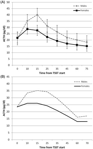
Overall, males had significantly higher ACTH levels during and after the TSST, sex effect F(1,69) = 5.77, p = 0.01, but this effect varied as a function of time, sex × time interaction F(1,368) = 3.14, p = 0.002. Specifically, males had significantly higher ACTH levels than females at 15 and 25 min after initiation of the task (Figure 2A).

Figure 2. ACTH changes in response to TSST for males and females modeled via repeated measures (A) and growth curve modeling (B). Repeated measures results show means and standard errors. Growth curve model shows estimated cubic curves. *Significant comparisons after Bonferroni adjustment.

AUCi and AUCg approach

Males had significantly higher total ACTH production after the stress task with respect to baseline (AUCi) (M = 384.17, SD = 702) than females (M = −105, SD = 779), t(51) = −2.36, p = 0.02. However, females (M = 1984.8, SD = 774) had greater total ACTH production with respect to ground than males (M = 1527, SD = 560), t(51) = −2.30, p = 0.02.

Growth curve modeling approach

We replicated these results via a non-linear (quadratic) growth curve model using the pre-TSST baseline sample as the intercept (non-adjusted data). We found no significant effect of sex on baseline levels, intercept F(1,51) = 0.001, p > 0.20, but a significant effect of sex on the non-linear trajectory, sex × time² effect F(1,365) = 5.28, p = 0.02, with males having significantly higher ACTH increases during the task (Figure 2B). We produced identical ACTH results when we replicated these analyses with the subset of participants (N = 42) who had salivary cortisol data available.

Sex differences in saliva cortisol response to the TSST

Repeated measures approach

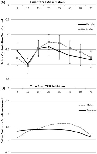
We found no overall differences in saliva cortisol between males and females, sex effect F(1, 40) = 0.66, p > 0.20, and no interaction between sex and time, sex × time interaction, F(1,240) = 0.76, p > 0.20 (Figure 3A). Further analyses of simple effects also confirmed no sex differences at any of the time points.

Figure 3. Saliva cortisol changes in response to TSST for males and females modeled via repeated measures (A) and traditional growth curve modeling (B). Repeated measures results show means and standard errors. Growth curve model shows estimated quadratic curves.

AUCi and AUCg approach

We found no significant difference in total cortisol production after stress (AUCi) between males (M = 2.79, SD = 1.45) and females (M = 3.31, SD = 1.48), t(40) = −1.14, p > 0.20. Likewise, there was no difference in AUCg between males (M = 2.92, SD = 1.46) and females (M = 3.40, SD = 1.48), t(40) = −1.05, p > 0.20.

Multilevel growth curve model from baseline (non-adjusted data)

An unconditional model shows that cortisol levels increased linearly, time b = 0.018, t(41) = 5.63, p < 0.001, but this increase decelerated with times, time² b = −0.0004, t(251) = −6.17, p < 0.001, reflecting the expected rise and eventual fall of cortisol after the TSST initiation. This quadratic model was the best fit to the data (AIC = 459 compared to linear = 492 and cubic = 461). In the conditional model, sex did not impact baseline levels, intercept b = 0.25, t(40) = 1.31, p = 0.20. However, sex impacted the cortisol trajectory. Specifically, females had a less steep linear increase, sex × time b = −0.23, t(290) = −3.59, p < 0.001, and a more gradual deceleration of cortisol changes, sex × time² b = 0.0002, t(290) = 3.09, p = 0.002 (Figure 3B). Given the shape of the estimated trajectories (Figure 3B), we calculated the estimated peak times for males and females from the growth trajectory estimates using the formula suggested by Singer & Willett (2003): Minutes to peak = −Rise/(2 × Curvature). Males had an estimated peak time at 38 min, while females peaked at 22 min, suggesting that females have a flatter trajectory while also peaking earlier than males.

Two-piece multilevel growth curve model without landmark registration

The unconditional time model indicated significantly increasing cortisol levels towards mean peak (activation slope), TimeBeforeGroupPeak b = 0.0013, t(175) = 4.20: p < 0.001, and significant decreasing cortisol levels after the peak (regulation slope), TimeAfterGroupPeak b = −0.011, t(124) = −6.04, p < 0.001. In the conditional model, sex did not significantly impact peak, Sex (male) b = 0.22, t(97.7) = 1.53, p = 0.13. Likewise, sex did not impact activation slope, Sex × TimeBeforeGroupPeak b = 0.002, t(174) = 0.38, p = 0.70, or regulation slope, Sex × TimeAfterGroupPeak b = −0.003, t(123) = −1.00, p = 0.31.

Two-piece multilevel growth curve model with landmark registration (adjusted time data)

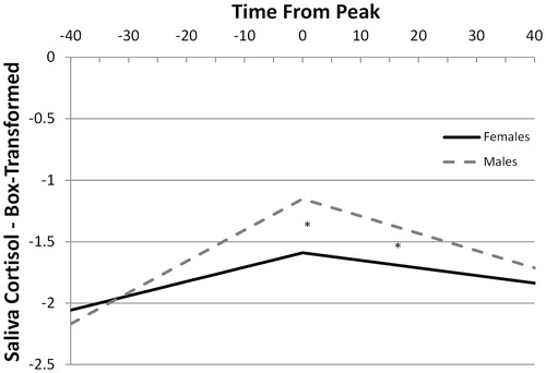
The unconditional time model indicated significantly increasing cortisol levels towards peak (activation slope), TimeBeforePeak b = 0.018, t(44.6) = 10.45, p < 0.001, and significantly decreasing cortisol levels after the peak (regulation slope), TimeAfterPeak b = −0.010, t(37.9) = −5.81, p < 0.001. There was also significant covariation between the peak (intercept), and both the activation, b = 0.01, z = 3.36, p < 0.001, and regulation slopes, b = −0.003, z = −2.63, p < 0.01, suggesting that greater peaks were associated with more positive activation slopes and more negative regulation slopes. In the conditional model, we found that males had significantly higher peak levels than females, Sex (male) b = 0.43, t(37) = 2.63, p = 0.01. Sex did not significantly impact the activation slope, Sex × TimeBeforePeak b = 0.0138, t(41.1) = 1.58, p = 0.12, but males had significantly steeper regulation slopes than females, Sex × TimeAfterPeak b = −0.0079, t(38.2) = −2.37, p = 0.02 (Figure 4). Since peak levels are a function of starting levels (baseline), intensity of activation (slope) and duration of activation (peak time), the differences in peaks without a significant difference in activation slope suggest that the groups differed in the duration of activation, with a more prolonged activation period producing later peaks in males. This is consistent with the estimated peak times obtained in the multilevel growth model without landmark registration and with the raw data in which males (M = 33.05, SD = 14) peaked on average 8 min later than females (M = 25, SD = 8.2). This difference approached significance t(28) = 1.92, p = 0.06.

Figure 4. Estimated saliva cortisol slopes before and after post-TSST peak for males and females modeled via growth curve modeling with landmark registered data (common peak). *Significant sex effect on peak and regulation slope, but not on activation slope.

Discussion

In this study, we present two-piece growth curve modeling with landmark registration as a complementary analytic approach when modeling salivary cortisol stress reactivity. This procedure partially controls for variability in the timing of the stress response, and can therefore identify individual and group differences in aspects of salivary cortisol stress reactivity that might be obscured by time-to-peak variability. It also allows a detailed examination of various phases of the post-stress response curves, which can provide additional insight into underlying biological processes driving individual and group differences in stress reactivity. Using this approach, we identified specific sex differences in salivary cortisol that were consistent with the ACTH differences observed in this sample, and that were otherwise missed by more traditional methods (i.e. examinations of time series means via repeated measures and examinations of area under the curve via t-tests). This result suggests that the proposed approach can provide neuroendocrine researchers with an additional tool to model stress reactivity that can be particularly useful when analyzing datasets that display significant variability in the timing of the post-stress peak response.

Using a two-piece GCM on a time adjusted database (landmark registration) we were able to simultaneously model sex differences in salivary cortisol at the post-stress peak, and in the slopes of cortisol towards (activation) and away (regulation) from the peak, while controlling for baseline levels and individual differences in the timing of the peak. We found that males had significantly higher post-stress salivary cortisol peaks than females but, paradoxically, the groups did not show a significant difference in the acceleration towards this peak. This discrepancy can reflect relatively parallel activation curves between males and females that differ in the timing of the peak, with males having a more prolonged stress response than females. This is in line with the overall pattern observed in ACTH (Figure 2A) in that both groups are relatively similar in their ACTH activation slopes but males continue on an upward slope after females’ levels started to decline. Furthermore, males showed a more intense down-regulation of the cortisol response than females (regulation slope), suggesting an intact regulatory capacity once salivary cortisol levels begin to decline. Yet, these differences are not apparent upon visual inspection of the non-adjusted saliva cortisol data (Figure 3A) because the average peak for males is not visible (mean = 33 min), which obscures both the peak and recovery slope differences. Notably, two of the three previous studies that also examined ACTH and salivary cortisol identified sex differences in ACTH but no differences in salivary cortisol using standard repeated measures ANOVA (Kirschbaum et al., 1999; Kudielka et al., 2004), a discrepancy that has been attributed to possible greater adrenal sensitivity in females (Horrocks et al., 1990; Roelfsema et al., 1993). However, previous results suggesting no sex differences in cortisol reactivity may be due to the use of analytical tools that are not sensitive to the type of differences noted in our study.

Definitive conclusions about the biological meaning of the differences detected are not possible from this single data set, but some speculative interpretations can illustrate the potential value of this approach. If males and females truly do have similar acceleration slopes (replication in a larger sample is needed to verify this), but males have prolonged activation, producing later peaks, followed by steeper regulation slopes, identification of underlying mechanisms may provide useful new information about stress response regulation differences between males and females. Prolonged activation could result from reduced sensitivity within the system’s inhibitory feedback components (e.g. glucocorticoid receptor sensitivity). However, steeper regulation slopes are inconsistent with this interpretation, as they suggest intact or enhanced feedback capacity, raising questions perhaps about male–female differences in activation threshold for feedback regulation, potentially due to differences in mineralocorticoid and glucocorticoid receptor numbers, ratios or distributions. Thus, it may be possible to derive more specific biological information from salivary cortisol growth curves through follow-up studies in which the analytic approaches described here are applied to larger samples in which additional laboratory probes are used to simultaneously provide more precise information about individual and group differences in specific HPA regulatory control components – e.g. central drive, feedback sensitivity, pituitary sensitivity, adrenal sensitivity. Such studies are underway.

We also found sex differences in salivary cortisol using traditional growth curve modeling even when we used the non-adjusted time data (i.e. not adjusting for phase variability in peak responses). This may be due to greater statistical power in growth modeling when analyzing time data compared to repeated measures, given that growth modeling correctly treats time as a continuous variable and thus does not result in the loss of power associated with categorizing time (Naggara et al., 2011). It is also possible that this approach is less susceptible to phase variability than repeated measures because growth modeling tests for deviations from an overall trajectory (mean curve) as opposed to differences at specific time-points (e.g. 25-min post-stress) which are likely more susceptible to phase variability. Yet, despite correctly identifying a sex difference, the information this model provided was arguably less informative as we can only make inferences about one group being more “reactive” as indicated by the non-linear parameters. That is, this modeling strategy does not allow us to determine whether the greater “reactivity” observed in the males is due to differences in the intensity of initial activation (slopes) or differences in the duration of the activation (peak latency), although the calculation of estimated peak times from the growth parameters can help researchers identify whether potential differences in peak latency may exist. Furthermore, the differences in trajectories implied by the estimated curves (Figure 3B) when using this approach do not appear to accurately represent the underlying salivary cortisol or ACTH data. These limitations are known problems when interpreting non-linear (e.g. quadratic, cubic) effects from a baseline, in that the non-linear parameters test for overall gross differences in the non-linear shape (e.g. “one group being flatter than another”), but do not readily provide information about group differences in specific aspects of the trajectories (e.g. peaks versus peak latency) without a complete reparameterization of the model (Cudeck & Toit, 2002). In contrast, the GCM with landmark registration suggest that the sex effect is likely a function of differences in peak latency as opposed to initial reactivity, which complements traditional GCM approaches and may add more precision to the modeling of salivary cortisol reactivity in cases of significant timing variability. Finally, we should note that a two-piece model using the mean sample peak timing as the intercept (without landmark registration) failed to identify the sex difference in peak levels or regulation slopes observed with the landmark registration. Thus, in the absence of landmark registration, a traditional growth curve model from baseline likely provides more accurate information than a two-piece model using average peak times.

Conclusions, limitations and recommendations

There are important limitations to the time-adjusted growth curve modeling approach, and to this study. Importantly, our study included a relatively small sample, which may have reduced power when using repeated measures and AUCi analyses. Yet, the fact that we identified sex differences in salivary cortisol when using GCM, paralleling results seen in temporally more precise ACTH data, highlights the robustness of this approach when applied to salivary cortisol, even with small samples. The use of landmark registration requires dense sampling of the post-stress slopes so that individual peaks closely approximate the true peak, which increases costs and participant demands. At a minimum, we recommend collecting samples at 0, 15, 25, 35, 45 and 60 min after the initiation of a task like the TSST. More frequent sampling (e.g. every 5 min) may be needed to model non-linear trajectories before and after the peak. However, even very frequent saliva sampling remains less invasive than the blood sampling required to obtain ACTH levels. This approach also requires significantly more data preparation, including the manual identification and validation of peak levels. It is likely that this process can be automated and there are algorithms that may be modified to serve this purpose (e.g. FindPeaks function in R). Furthermore, this approach led to significant covariation between the slopes and intercept (peak) potentially leading to multicollinearity, which can increase standard errors and make it more difficult to find significant effects (Alin, 2010). High intercept-slope covariance is a known issue in growth curve modeling when the time variable is re-centered (Biesanz et al., 2004). However, there is debate about whether such covariation is a problem in growth modeling when it is due to re-centering of the time variable (Biesanz et al., 2004). Nonetheless, users of this approach should be cognizant of the potential intercept-slope covariation and its potential impact on standard errors. Finally, this approach does not fully separate phase and amplitude effects because there are common factors that impact both effects (e.g. feedback inhibition), so users should use caution when interpreting results as reflection of purely phase or amplitude variability.

Our approach partially controls for phase variability and allows us to more clearly “see” aspects of response curves that may be important to fully understand the biologically shaped activation and regulation. This approach may be particularly useful in HPA axis studies because there can be wide individual and group variation in sensitivity to contextual and anticipatory aspects of study paradigms – for some the cortisol response can begin well before the experimentally-controlled “stressor” is applied (Alpers et al., 2003) – and in some studies a prolonged series of stressors may be utilized in a way that adds substantial noise to phase-related variables. As a result, approaches that allow better control over timing differences may provide greater insight into other important aspects of regulatory control in stress response systems. However, blindly using this approach alone, without at least visually inspecting the overall patterns of the unadjusted data and applying more traditional methods when indicated, could lead researchers to miss important phase variability differences that may also be biologically important (e.g. Figure 1A). Thus, we view this approach as complementary to traditional approaches, and in some cases, combining approaches can help us understand and tease apart amplitude and phase variability in neuroendocrine stress paradigms, perhaps with potential to reduce some of the inconsistencies that have plagued this literature for years.

In sum, common analytic approaches used to examine cortisol reactivity (e.g. rANOVA of time series means, examinations of AUCi) do not account for individual and group differences in the timing of cortisol response and thus may lack sensitivity to identify subtle differences in cases of significant phase variability. Likewise, these approaches often provide basic estimations of post-stress cortisol differences that are not easily translated to key parameters that could inform the underlying biological processes (e.g. intensity of activation and regulation). Growth curve modeling with landmark registration is an accessible analytic approach based on common statistical tools that can address these limitations by partially accounting for differences in the timing of response and providing easily interpretable estimations of activation and regulation slopes and peaks. This approach allows researchers to examine the dynamics of the cortisol response in a way that adds to, and in some ways may improves upon, what is available with more common analytic tools.

Declaration of interest

The authors report no conflicts of interest. The authors alone are responsible for the content and writing of this article.

Acknowledgements

We would like to thank David Childers and Kathleen Welch at the University of Michigan Center for Statistical Consultation and Research for providing valuable feedback about our statistical approach.

References

- Abelson JL, Erickson TM, Mayer SE, Crocker J, Briggs H, Lopez-Duran NL, Liberzon I. (2014). Brief cognitive intervention can modulate neuroendocrine stress responses to the Trier Social Stress Test: buffering effects of a compassionate goal orientation. Psychoneuroendocrinology 44:60–70
- Abelson JL, Khan S, Liberzon I, Erickson TM, Young EA. (2008). Effects of perceived control and cognitive coping on endocrine stress responses to pharmacological activation. Biol Psychiatry 64:701–7
- Alin A. (2010). Multicollinearity. Wiley Interdiscip Rev Comput Stat 2:370–4
- Alpers GW, Abelson JL, Wilhelm FH, Roth WT. (2003). Salivary cortisol response during exposure treatment in driving phobics. Psychosom Med 65:679–87
- Bellgowan PSF, Saad ZS, Bandettini PA. (2003). Understanding neural system dynamics through task modulation and measurement of functional MRI amplitude, latency, and width. Proc Natl Acad Sci USA 100:1415–19
- Biesanz JC, Deeb-Sossa N, Papadakis AA, Bollen KA, Curran PJ. (2004). The role of coding time in estimating and interpreting growth curve models. Psychol Methods 9:30–52
- Burson A, Crocker J, Mischkowski D. (2012). Two types of value-affirmation: implications for self-control following social exclusion. Soc Psychol Personal Sci 3:510–16
- Childs E, Dlugos A, De Wit H. (2010). Cardiovascular, hormonal, and emotional responses to the TSST in relation to sex and menstrual cycle phase. Psychophysiology 47:550–9
- Clements AD. (2013). Salivary cortisol measurement in developmental research: where do we go from here? Dev Psychobiol 55:205–20
- Cudeck R, Toit SHC. (2002). A version of quadratic regression with interpretable parameters. Multivariate Behav Res 37:501–19
- De Kloet ER. (2004). Hormones and the stressed brain. Ann N Y Acad Sci 1018:1–15
- Gasser T, Kneip A, Ziegler P, Largo R, Prader A. (1990). A method for determining the dynamics and intensity of average growth. Ann Hum Biol 17:459–74
- Gueorguieva R, Krystal JH. (2004). Move over ANOVA: progress in analyzing repeated-measures data and its reflection. Arch Gen Psychiatry 61:310–17
- Hellhammer DH, Wüst S, Kudielka BM. (2009). Salivary cortisol as a biomarker in stress research. Psychoneuroendocrinology 34:163–71
- Horrocks P, Jones A, Ratcliffe W, Holder G, White A, Holder R, Ratcliffe J, London D. (1990). Patterns of ACTH and cortisol pulsatility over twenty-four hours in normal males and females. Clin Endocrinol (Oxf) 32:127–34
- Hruschka DJ, Kohrt BA, Worthman CM. (2005). Estimating between- and within-individual variation in cortisol levels using multilevel models. Psychoneuroendocrinology 30:698–714
- Jansen B, Huang H. (1985). Automated morphological analysis by means of dynamic time-warping. Electroencephalogr Clin Neurophysiol 60:282–4
- Kirschbaum C, Hellhammer D. (1989). Salivary cortisol in psychobiological research: an overview. Neuropsychobiology 22:150–69
- Kirschbaum C, Kudielka BM, Gaab J, Schommer NC, Hellhammer DH. (1999). Impact of gender, menstrual cycle phase, and oral contraceptives on the activity of the hypothalamus-pituitary-adrenal axis. Psychosom Med 61:154–62
- Kirschbaum C, Pirke KM, Hellhammer DH. (1993). The trier social stress test – a tool for investigating psychobiological stress responses in a laboratory setting. Neuropsychobiology 28:76–81
- Kirschbaum C, Pirke KM, Hellhammer DH. (1995). Preliminary evidence for reduced cortisol responsivity to psychological stress in women using oral contraceptive medication. Psychoneuroendocrinology 20:509–14
- Kirschbaum C, Wolf OT, May M. (1996). Stress- and treatment-induced elevations of cortisol levels associated with impaired declarative memory in healthy adults. Life Sci 58:1475–83
- Kirschbaum C, Wüst S, Hellhammer DH. (1992). Consistent sex-differences in cortisol responses to psychological stress. Psychosom Med 54:648–57
- Kneip A, Gasser T. (1992). Statistical tools to analyze data representing a sample of curves. Ann Stat 20:1266–305
- Kudielka BM, Buske-Kirschbaum A, Hellhammer DH, Kirschbaum C. (2004). HPA axis responses to laboratory psychosocial stress in healthy elderly adults, younger adults, and children: impact of age and gender. Psychoneuroendocrinology 29:83–98
- Kudielka BM, Hellhammer DH, Wüst S. (2009). Why do we respond so differently? Reviewing determinants of human salivary cortisol responses to challenge. Psychoneuroendocrinology 34:2–18
- Kumsta R, Entringer S, Hellhammer DH, Wüst S. (2007). Cortisol and ACTH responses to psychosocial stress are modulated by corticosteroid binding globulin levels. Psychoneuroendocrinology 32:1153–7
- Lindquist MA, Meng Loh J, Atlas LY, Wager TD. (2009). Modeling the hemodynamic response function in fMRI: efficiency, bias and mis-modeling. Neuroimage 45:S187–98
- Lopez-Duran NL, Hajal NJ, Olson SL, Felt BT, Vazquez DM. (2009). Individual differences in cortisol responses to fear and frustration during middle childhood. J Exp Child Psychol 103:285–95
- Matthews JN, Altman DG, Cambell MJ, Royston P. (1990). Analysis of serial measurements in medical research. Br Med J 300:230–5
- Miller R, Plessow F. (2012). Transformation techniques for cross-sectional and longitudinal endocrine data: application to salivary cortisol concentrations. Psychoneuroendocrinology 38:941–6
- Naggara O, Raymond J, Guilbert F, Roy D, Weill A, Altman DG. (2011). Analysis by categorizing or dichotomizing continuous variables is inadvisable: an example from the natural history of unruptured aneurysms. Am J Neuroradiol 32:437–40
- Pruessner JC, Kirschbaum C, Meinlschmid G, Hellhammer DH. (2003). Two formulas for computation of the area under the curve represent measures of total hormone concentration versus time-dependent change. Psychoneuroendocrinology 28:916–31
- Ramsay J. (2006). Functional data analysis. 2nd ed. New York, NY: Springer
- Ramsay JO, Li X. (1998). Curve registration. J R Stat Soc Ser B (Statistical Methodol) 60:351–63
- Roelfsema F, Van G, Berg M. (1993). Sex-dependent alteration in cortisol response to endogenous adrenocorticotropin. Pituitary 77:234–40
- Rohleder N, Schommer NC, Hellhammer DH, Engel R, Kirschbaum C. (2001). Sex differences in glucocorticoid sensitivity of proinflammatory cytokine production after psychosocial stress. Psychosom Med 63:966–72
- Schlotz W, Hammerfald K, Ehlert U, Gaab J. (2011). Individual differences in the cortisol response to stress in young healthy men: testing the roles of perceived stress reactivity and threat appraisal using multiphase latent growth curve modeling. Biol Psychol 87:257–64
- Schoofs D, Wolf OT. (2011). Are salivary gonadal steroid concentrations influenced by acute psychosocial stress? A study using the Trier Social Stress Test (TSST). Int J Psychophysiol 80:36–43
- Singer JD. (1998). Using SAS PROC MIXED to fit multilevel models, hierarchical models, and individual growth models. J Educ Behav Stat 23:323–55
- Singer JD, Willett J. (2003). Applied longitudinal data analysis: modeling change and event occurrence. New York, NY: Oxford University Press
- Uhart M, Chong RY, Oswald L, Lin P-I, Wand GS. (2006). Gender differences in hypothalamic-pituitary-adrenal (HPA) axis reactivity. Psychoneuroendocrinology 31:642–52
- Vantini S, Vatini S. (2012). On the definition of phase and amplitude variability in functional data analysis. Test 21:676–96
- Wang K, Begleiter H, Porjesz B. (2001). Warp-averaging event-related potentials. Clin Neurophysiol 112:1917–24
- Wu S, Jude S. (2010). Two-piecewise random coefficient model using proc mixed. PharmaSUG Conf Proc. p 1–6