A factor analysis of the SSQ (Speech, Spatial, and Qualities of Hearing Scale)

Abstract

Objective: The speech, spatial, and qualities of hearing questionnaire (SSQ) is a self-report test of auditory disability. The 49 items ask how well a listener would do in many complex listening situations illustrative of real life. The scores on the items are often combined into the three main sections or into 10 pragmatic subscales. We report here a factor analysis of the SSQ that we conducted to further investigate its statistical properties and to determine its structure. Design: Statistical factor analysis of questionnaire data, using parallel analysis to determine the number of factors to retain, oblique rotation of factors, and a bootstrap method to estimate the confidence intervals. Study sample: 1220 people who have attended MRC IHR over the last decade. Results: We found three clear factors, essentially corresponding to the three main sections of the SSQ. They are termed “speech understanding”, “spatial perception”, and “clarity, separation, and identification”. Thirty-five of the SSQ questions were included in the three factors. There was partial evidence for a fourth factor, “effort and concentration”, representing two more questions. Conclusions: These results aid in the interpretation and application of the SSQ and indicate potential methods for generating average scores.

Key Words::

• Psychoacoustics/hearing science
• behavioral measures
• hearing aids
• speech perception

Abbreviations
IHR	=	Institute of Hearing Research
MRC	=	Medical Research Council
SSQ	=	Speech, spatial, and qualities of hearing scale

Gatehouse and Noble's Speech, Spatial, and Qualities of Hearing Scale (SSQ) is a 49-item self-assessment questionnaire of hearing disability (Gatehouse & Noble, 2004; Noble & Gatehouse, 2004, 2006)¹. Each item asks how well a listener would do in a vignette of one of the myriad complex listening situations typical of real life. The SSQ is an intermediate link between the audiological measurement of someone's hearing loss (i.e. their impairment) and a patient's assessment of how that hearing loss impacts their wider life (i.e. their handicap, or participation restriction). The SSQ has been used in studies assessing the effects of bilateral hearing aids (e.g. Ahlstrom et al, 2009; Kobler et al, 2010; Most et al, 2012; Noble and Gatehouse, 2006), cochlear implants (e.g. Tyler et al, 2009), cochlear implants in one ear and hearing aids in the other (Potts et al, 2009), bone-anchored hearing aids (e.g. Martin et al, 2010; Wieringen et al, 2011), the surgical removal of acoustic neuromas (Douglas et al, 2007), and investigations of older and younger adults with normal audiometric values (Banh et al, 2012). Shortened forms have been developed (e.g. Akeroyd and Guy, 2011; Helfer et al, 2009; Demeester et al, 2012; Keidser et al, 2009; Kiessling et al, 2011; Odelius and Johansson, 2010; Noble et al, 2012, 2013); there are translations into Arabic, Danish, Dutch, German, and Swedish (Kiessling et al, 2011; Kobler et al, 2010; Most et al, 2012; van Wieringen et al, 2011), and a parental version has been developed (Galvin et al, 2007, 2010). There are also two versions designed for directly measuring the benefit of an intervention or the comparison of one intervention with another, namely SSQ-B and SSQ-C (Jensen et al 2009).

Two general approaches have been taken when reporting SSQ data. Gatehouse and Noble reported SSQ statistics at the level of individual items, averages across all the items in each of the three sections, and the grand averages across all items in the questionnaire. Many of the subsequent SSQ studies cited above also reported their data in these ways (e.g. Tyler et al, 2009). The other approach has been to use the ten “pragmatic” subscales developed by Gatehouse and Akeroyd (2006) (e.g. Ahlstrom et al, 2009; Most et al, 2012; Noble et al, 2008, 2012). These were designed for data reduction, based on a reasoned interpretation of the import of the questions not their statistical or psychometric properties.

The statistical properties of the SSQ have been considered in two previous studies. First, Singh and Pichora-Fuller (2010) reported test-retest data for 159 older adults (mean age = 73 years; mean better-ear hearing loss = 18 dB HL). The tests were made about six months apart. They found that the test-retest correlation of the whole questionnaire was 0.83 when both the test and retest SSQs were administered by interview with a trained member of staff, but was 0.65 when the SSQs were instead self-administered using a form mailed to each participant. They reported values of Cronbach's alpha (a measure of internal reliability) for the whole questionnaire of 0.96–0.97 for both tests by interview, though again it was smaller, at 0.88–0.93, for both tests by mail. Second, Demeester et al (2012) reported a value of Cronbach's alpha of 0.96 for SSQ data collected on three groups of participants, totaling 236 people (the three groups were younger normal hearing, older normal and older with a hearing loss, with mean four-frequency hearing losses of the groups of 8, 17, and 22 dB HL, respectively; the SSQ was self-administered by participants but the responses were subsequently checked and if necessary explained). Demeester et al also conducted a cluster analysis of their data for the purposes of reducing the SSQ to a short screening instrument. To do this they set the number of clusters to be five, so, in essence, they were forcing the SSQ items into five separate groups. They found that three of the clusters essentially represented the speech, space, and qualities sections: one cluster had nine of the speech-section items but no others, a second cluster had 16 of the spatial-section items though it also had two of the qualities-section items, a third cluster had seven of the qualities-section items but no others. The two remaining clusters were mixed: one was an eight-item group across all three sections, the other was a three-item group across two sections.

Here we report a factor analysis of SSQ data from 1220 adults with a range of ages and hearing losses, taking advantage of 10 years of SSQ data that we have been collecting in our laboratory for other purposes. The results of the factor analysis—especially how many factors there are and which items load on which factors— help in understanding the structure of the SSQ and may be of assistance in developing new forms; for instance, they were included in the development of the SSQ-12 (Noble et al, 2013).

Methods

Data collection

The data were collected during visits by patients and others to the MRC IHR, from 2002 to Dec 2011. Generally the patients were sourced from NHS Audiology at Glasgow Royal Infirmary. Audiograms were measured using standard UK methods. Though we had audiogram data on 1726 people, the analyses were run on data from those 1220 participants on whom we had complete data for an air-conduction audiogram (250, 500, 1000, 2000, 3000, 4000, 6000, and 8000 Hz, in both ears), a bone-conduction audiogram (500, 1000, 2000, 3000, and 4000 Hz, in both ears), the SSQ, and the 12-question hearing handicap questionnaire (Gatehouse and Noble, 2004).

The SSQ data were collected by interview with trained IHR staff. About half the data (up to Spring 2008) was collected using a paper form. The subsequent data was collected using a computerized form. The paper form is illustrated in Appendix 1 of Gatehouse and Noble; the computer version was programmed to be visually similar. Each question was read to the participant, and then they were asked to give a response, ranging from 0 to 10, corresponding to “not at all” and “perfect” (though some items had different labels: see Appendix 1 of Gatehouse & Noble, 2004). Further explanations of the items were given if necessary. In both the paper and computer questionnaires the response scales were continuous, but with integer divisions prominently marked. To simplify subsequent data analysis and presentation, any responses that were not to either integers or half-integers (i.e. x.5) were rounded accordingly. Across everyone the ratio of integer to half-integer responses was 6.3:1.

It was not compulsory to respond to every question: sometimes people said that a particular question was not applicable to them or otherwise did not respond². The missing-response rates were less than 2.5% for all questions but Speech #7, Space #5, #14, #15, #16, Qualities #15, #16, for which the rates were, respectively, 3.0%, 2.8%, 12.3%, 4.8%, 5.3%, 55.9%, and 45.2%. As the missing- response rates for Qualities questions #15 and #16 were about a magnitude larger than those for any other question, they were entirely removed from the analyses: we presume the high missing-response rates were because they are only applicable in particularly specific situations [respectively, they are “If you turn one hearing aid/implant off, and do not adjust the other, does everything sound unnaturally quiet?” and “When you are the driver in a car can you easily hear what someone is saying who is sitting alongside you?”]. This left 48 questions: 14 in the Speech section, 17 in the Spatial section, and 17 in the Qualities section. The average score across all 48 questions is termed “SSQ₄₈”³.

Classification of participants

We calculated the better-ear hearing loss as the mean of the air-conduction hearing levels at 500, 1000, 2000, and 4000 Hz in each participant's better ear. For many of the analyses the 1220 participants were divided into three classes of hearing-aid fitting: unaided, unilaterally aided, and bilaterally aided. The rationale for this division is that their responses were based on how they listened in their everyday life: if they wore hearing aids in everyday life, then they responded on the basis of their aided listening (note that other divisions of the participant are considered in the Discussion). The group sizes were, respectively, 386, 627, and 207 (see Table 1); the median ages were 58, 65, 64 years; the median better-ear hearing losses were 31, 44, 56 dB HL; the median worse-ear hearing losses were 32, 56, and 66 dB HL. The distributions of age and better-ear hearing loss are plotted in Figure 1.

Figure 1. Distributions of better-ear hearing loss (top panel) and age (bottom panel) for the 1220 participants. The hearing loss is calculated as the mean of the air-conduction hearing levels at 500, 1000, 2000, and 4000 Hz in a participant's better ear. They are grouped into 10-dB bins; age is grouped into decade bins. The hatchings mark the three groups of listeners.

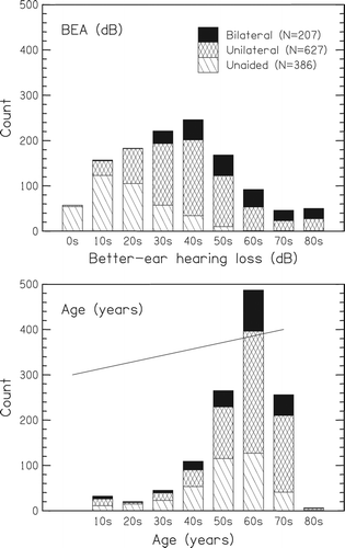
Table 1. The counts, age, and hearing losses of the three groups of listeners. The values are means with medians in brackets.

			Age	Left 4FA	Right 4FA	BEA	WEA
Group	N	Males:females	years	dB	dB	dB	dB
Unaided	386	190 : 196	54 (58)	29 (28)	28 (25)	23 (21)	35 (32)
Unilaterally aided	627	319 : 308	61 (65)	53 (50)	52 (49)	44 (44)	60 (56)
Bilaterally aided	207	89 : 118	58 (64)	63 (60)	62 (61)	58 (56)	67 (66)
Everyone	1220	598 : 622	59 (63)	47 (45)	46 (45)	40 (39)	53 (51)

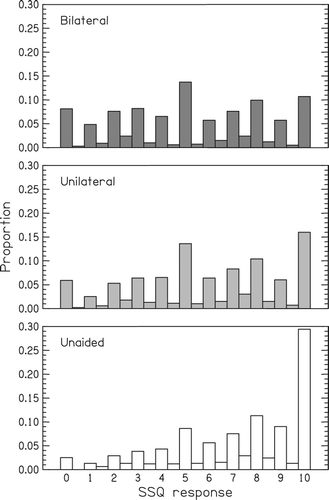
Figure 2 shows the distribution of SSQ responses for the three groups. The preference towards responding with integers as against half-integers is clear. The response distributions for the bilateral and unilateral groups were reasonably even across the 0–10 range, excepting slight biases towards responding 5 or 10 and away from responding 9 or 1. For the unaided group, however, there was a large bias towards responding 10 (= 29% of all responses).

Figure 2. Distributions of the responses to each possible point on the SSQ scale across all 1220 participants times 48 questions. The three groups are for unaided listeners (n = 386), unilaterally aided (n = 627), and bilaterally aided (n = 207). Any non-integer (or half-integer) responses have been rounded to the nearest integer (or half integer).

Figure 3 plots the SSQ₄₈ score against deciles of better-ear hearing loss. There was a general negative relationship: the linear regression relating an individual's SSQ₄₈ score to their hearing loss (HL), across all 1220 participants, was

Figure 3. Mean SSQ score vs. better-ear hearing loss. The listeners are grouped by aiding configuration (top panel) or age (bottom panel). The score is the average response across the 48 SSQ questions considered here. In the top panel the error bars in the top-right corner illustrate the minimum, mean, and maximum standard deviations of the data points. See Figure 1 for the calculation of hearing loss.

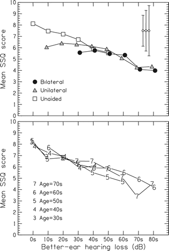
which accounted for 21% of the variance in the individual data and 85% of the variance in the grouped data shown in the top panel of Figure 3. There were secondary effects of aiding type at low losses (top panel) or age at high losses (bottom panel)⁴.

Factor analysis procedures

For the main factor analyses we chose these options: un-transformed data; factor extraction using common factor analysis by maximum likelihood; three factors retained through a parallel analysis; oblique rotation. The rationales for each of these choices are outlined in the following paragraphs. The factor analyses were run in PASW (SPSS) version 18 using the “Factor” subroutine. The input was the 48 × 48 matrix of Pearson cross-correlations of SSQ questions calculated in Matlab, rather than the 1220 × 48 matrix of actual SSQ responses⁵. This was done in order to allow random datasets to be easily constructed in Matlab for the parallel analysis and for a subsequent bootstrap procedure. The correlation matrices were calculated to six decimal places to minimize loss of accuracy in the intermediate step of copying the matrix from one program to another. The factor weightings reported below are the values in the pattern matrix returned by Field (2009) and Tabachink and Fidell (2007). The pattern matrix records the unique contribution of each variable to the factor. The alternative, the structure matrix, is confounded by incorporating the correlations between each factor.

As there is a very large literature on factor analysis since its invention by Spearman (1904) the citations are selective rather than exhaustive. We have found the following to be informative as they discuss many of the issues in depth: the papers by Floyd & Widamen (1995), Fabrigar et al (1999), Preacher & MacCallum (2003), Pohlmann (2004), and Costello & Osborne (2005), the relevant chapters in the books by Stevens (1996), Tabachnick & Fidell (2007), and Field (2009), and the full books by Carroll (1993) and Cudeck & MacCallum (2007),

The decision not to transform the data was based on the distributions of responses (Figure 2). Though the distribution for the unaided group was clearly skewed to high responses, the distributions for the unilateral and bilateral groups were more even. The overall descriptive statistics of the SSQ responses, across all participants and questions (i.e. n = 1220 × 48 = 58560), were mean = 6.2, standard deviation = 3.0, skewness = − 0.4, and excess kurtosis = 0.02. Given that the skewness was not too large, the excess kurtosis was very close to zero, and the above-noted broad characteristics in the response distributions, we felt that any transformation would have been minor in effect and moreover likely open to debate as to choice. Also, it is not formally required for a factor analysis that the data be normally distributed (Tabachink & Fidell, 2007): though normally distributed data is required if statistical significance tests or confidence intervals are to be calculated, we assessed the reliability of the results using a bootstrap method (see below).

The minimum group size for factor analysis has been discussed often (e.g. Guadagnoli & Velicer, 1988; MacCallum et al, 1999). A typical rule-of thumb for sample sizes is that they should number in the hundreds (Comrie & Lee, 1992; Tabachnick & Fidell, 2007). Another popular rule is that there should be about 5–10 participants per variable (Kass & Tinsley, 1979), though Guadagnoli and Velicer (1988) discounted this method. Kaiser (1970) defined an index of sampling adequacy, now generally named the Kaiser-Meyer-Olkin measure, such that values in the 0.90s represented “really excellent data” (p. 405). Numerical studies have shown that the recommended minimum number of participants depends somewhat on the number and strength of variables loading on a factor (Field, 2007): Guadagnoli and Velicer (1988) recommended around 150 would be sufficient if there were around 10–12 variables loading on factors with loadings as low as 0.4. Our group sizes were 207, 386, and 627. These correspond to 4.3–13 participants per variable. In Comrie and Lee's (1992) grading these would be “fair”, “good”, and “very good”. The Kaiser-Meyer-Olkin values for our data were 0.95–0.97 across the three groups. As is reported below in the analyses, we found 13–14 items per factor with loadings of at least 0.4. Taken all together, we therefore regard our group sizes as adequate. We note in passing that Gatehouse and Noble (2004) did not report a factor analysis as their dataset was too small, and commented that their small sample (n = 153) did not give stable results. They suggested that about 500 observations would be needed.

There are two general methods for extracting factors: principal components analysis (PCA) and common (or principal) factor analysis. The two approaches differ in their purposes. The goal of the former is essentially mathematical data reduction: “to explain as much of the variance in the matrix of raw scores as possible in the lowest possible rank (or the minimum number of dimensions)” (Widamark, 2007, p. 183). The goal of the latter is essentially to gain insight into the underlying structure: “to explain off-diagonal correlations among manifest variables, by positing the presence of one or more latent variables that represent the correlations amongst manifest variables” (Widamark, 2007, p. 182). We therefore chose common factor analysis, as our present aim was to determine any underlying structures of the SSQ questionnaire rather than conduct a data reduction exercise. There appears to be no consensus as to the best algorithm for extracting common factors, however, and so of the various choices available we adopted maximum likelihood as it is generally well-received (e.g. Costello & Osborne, 2005).

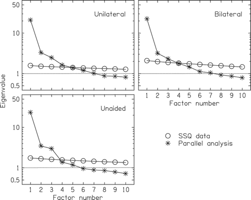
As the factor analyses were run on a 48 × 48 matrix of question-by-question correlations, each returns 48 factors, which are reported in order of decreasing eigenvalue. The mathematics of factor analysis requires that all 48 factors taken together are required to account for the whole data, but generally only the first few factors account individually for substantial amounts of variance, and therefore it is usual to keep only a small number before undertaking the rotation. A popular option, perhaps because it is the default in many statistics programs, is to keep only those factors whose eigenvalues are larger than 1. This is also known as the Kaiser criterion (Kaiser, 1960). An alternative is to plot the eigenvalue versus factor number, and only keep those factors to the left of the break in the slope of the plot. This is Cattell's “scree test” (Cattell, 1966; Cattell & Vogelmann, 1977). But both of these have often been criticized: the Kaiser criterion often gives too many factors, and the scree test is essentially a “rule of thumb” as one cannot be certain where the scree starts (e.g. Zwick & Velicer, 1986; Velicer & Jackson, 1990; Floyd Widamen, 1995; Fabrigar et al, 1999; Hayton et al, 2004). Accordingly, we chose a third option, parallel analysis (Horn, 1965). This has received increasing attention in recent decades as computers have become powerful enough to run it, and various commentators have commended it (e.g. Zwick & Velicer, 1986; Thompson & Daniel, 1996; Hayton et al, 2004; Dinno, 2009). The essence of parallel analysis is that one only keeps factors that are unlikely to have arisen by chance. The first stage of the procedure is to draw random numbers from a distribution whose characteristics match the experimental data: i.e. for our unaided group, we drew 386 independent sets of 48 independent random numbers, with the underlying distribution of random numbers set identical to the observed distribution shown in Figure 2 (the process for the unilateral and bilateral data was the same, expect that the underlying distributions for the random datasets matched their distributions and the number generated matched their sample sizes of 627 and 207). The 48 × 48 correlation matrix is then calculated and a factor analysis applied to it. If the random data were ideal, then the correlation table would be full of zeros and all the eigenvalues of the factors would be 1.0. But because the random data is only sampled from a random distribution, the correlations will only be distributed around zero instead of all being exactly zero, and so the eigenvalues will be distributed around 1. Thus some factors will have eigenvalues larger than 1, some less than 1. The process is repeated a large number of times (in our case, 50) and the mean eigenvalues of each factor calculated. These are the eigenvalues of entirely random data. If the eigenvalue of the nth factor in the observed data is less than or about the same as that of the nth factor in the random data, then it could have arisen by chance: but if the eigenvalue of the nth factor in the observed data is larger than that of the nth factor in the random data then it is unlikely to have arisen by chance. One therefore only keeps the first N observed factors whose eigenvalues are larger than those from the first N random factors. The results of the parallel analysis for each of the participant groups are shown in Figure 4. It can be seen that only the first three observed factors (asterisks) in all groups consistently gave eigenvalues larger than those from the random data (circles). Thus we retained three factors for the rotation and reporting in the main analyses. For factor #4 only one out of the three eigenvalues of the observed data was larger than the eigenvalues of the random data. This is considered further in the Discussion.

Figure 4. The results of the parallel analysis for determining the number of factors to retain. The circles plot the eigenvalues from the data; the asterisks from random distributions. The three panels are for the separate analyses for the three groups of listeners.

Factor rotation is necessary as the initial solution returned by the factor-analysis algorithm is indeterminate: if the n retained factors are regarded as defining the axes of a n-dimensional space, than any geometrical transformation of that space will give a solution that works exactly as well as the initial solution. The initial solution lists factors in decreasing order of eigenvalue (or, equivalently, percentage variance accounted for, as the two are related). The first factor found accounts for as much as possible of the variance, the second factor accounts for as much as possible of what variance remains, and so on. In general it is found that the first factor accounts for the vast majority of variance and the others far less. It is usual to rotate the results to give more equal amounts of variance. The rotated structure is mathematically equivalent to the initial structure but it is easier to interpret scientifically (e.g. Thurstone, 1935; Browne, 2001; Jennrich, 1979, 2007). An orthogonal rotation (which again is the default in many programs) assumes that the factors are completely independent—i.e. geometrically orthogonal—to each other. This is a priori unlikely for auditory disability: it requires that were there to be multiple factors of disability then someone's score on the first factor would be entirely unrelated to their score on the second factor, and so on. Instead it is much more likely that the factors will be somewhat linked, and so will show a non-zero correlation. An oblique rotation allows for this. Also, it is more general: if the factors really are orthogonal, then the oblique rotation will return that. The particular rotation chosen here was “direct oblimin” in PASW, with the delta parameter set to the default value of 0.0. To minimize confusion we use the notation F₁, F₂, F₃ to refer to the unrotated factors and F_SU, F_SP, F_CSI to refer to the rotated factors; the subscripts are the abbreviations of the factor names (see subsection headings below).

Results

Communalities

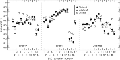
Figure 5 shows the communalities of the questions for each of the unaided, unilateral, and bilateral analyses (respectively, open squares, shaded triangles, and filled circles). The communality for each question is the across-factor sum of the squared loading, so indicates the amount of variance in each that is accounted for by the three retained factors. It can be seen that in general the communalities were respectable and that the values from the three analyses were in agreement. The mean communalities for the three groups were 0.60, 0.53, and 0.56, respectively (standard deviations across items = 0.14, 0.17, and 0.17). We note that the communalities were very low for three Space questions (#14, #15, and #16), indicating that the factors did a poor job of accounting the variance in them. Questions #14 deals with the externalization or internalization of sounds, a topic considerably different to that of the rest of the Space questions (“Do the sounds of things you are able to hear seem to be inside your head rather than out there in the world?”), whereas questions #15 and #16 are explicitly about perceived distance and how well it matches one's expectations (“Do the sounds of people or things you hear, but cannot see at first, turn out to be closer than expected when you do see them?” and “Do the sounds of people or things you hear, but cannot see at first, turn out to be further away than expected when you do see them?”). That there are two other questions about perceived distance that gave a much higher communality suggest that the effect was not due to distance per se (Spatial #8 and #9: “In the street, can you tell how far away someone is, from the sound of their voice or footsteps?”, and “Can tell how far away a bus or a truck is, from the sound?”). These three Space questions are returned to below.

Figure 5. The communalities of the 48 SSQ items. The symbols mark the three groups of listeners.

Overview of factors

Table 2 reports the overall variance-accounted-for results of the factor analyses. The five middle columns report the data for the first five unrotated factors. The reader is reminded that the process of factor analysis returns factors in order of decreasing variance accounted for before the rotations: F₁ accounts for as much as possible of the variance, F₂ that accounts for as much as possible of what variance is left, and so on. The general reduction of variance across from factor F₁ to factor F₅ was therefore expected. That the amount of variance accounted for by factors F₄ and F₅ was no more than 4% provides additional support for the decision to retain just the first three. The three rightmost columns report the squared loadings of the three rotated factors F_SU, F_SP, and F_CSI. F_SU and F_SP were about equal to one another, though F_CSI was slightly less. Table 3 reports the cross-correlations between the factors. They were substantial—between 0.5 and 0.7—so indicating that choosing an orthogonal rotation on the assumption that the factors were independent would have been unwelcome.

Table 2. Results of the factor analyses: amount of variance accounted for by each of the unrotated or rotated factors.

	Initial percentage of variance (unrotated factors)					Rotation sums of squared loadings (rotated factors)
Group	#1	#2	#3	#4	#5	FSU	FSP	FCSI
Unaided	49.1%	7.2%	6.2%	2.8%	2.5%	18.4	19.4	14.6
Unilaterally aided	44.0%	6.8%	5.1%	3.4%	2.9%	15.6	17.0	16.1
Bilaterally aided	47.0%	6.6%	4.8%	3.7%	3.0%	16.9	17.9	17.1

Table 3. Results of the factor analyses: Correlations of each rotated factor with each other.

	Factor correlations (rotated factors)
Group	FSU × FSP	FSU × FCSI	FSP × FCSI
Unaided	0.66	0.52	0.58
Unilaterally aided	0.61	0.62	0.68
Bilaterally aided	0.60	0.63	0.66

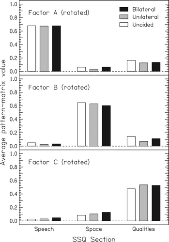
Figure 6 shows the mean factor weightings (i.e. the pattern matrix) for each group and factor, averaged across each of the three sections of SSQ questions (e.g. the left-most bar in the top panel is the mean value for F_SU across the 14 questions in the Speech section for the unaided group). It is clear that F_SU essentially represents the Speech questions, F_SP essentially represents the Space questions, and F_CSI essentially represents the Qualities questions. That this is a particularly simple pattern to interpret again supports the decision of keeping three factors. Each factor is considered separately below.

Figure 6. The mean factor weightings for each of the three retained factors, after oblique rotation. The weightings are averaged across all the items in a particular section of the SSQ. The hatchings mark the three groups of listeners.

F_SU = “Speech Understanding”

The top panel of Figure 7 shows the factor weighting values for F_SU for each of the unaided, unilateral, and bilateral groups (respectively, open squares, shaded triangles, and filled circles). There is little difference between the results for the three groups. It is clear that F_SU loads primarily on the questions in the Speech section but without making much distinction between them – though with a few exceptions discussed in the next paragraphs. This factor is therefore interpreted as being one of general speech understanding.

Figure 7. The factor weightings for each of the 48 SSQ items in each of the three factors. The symbols mark the three groups of listeners. The top panel shows the first rotated factor, named “Speech understanding”, the middle panel shows the second rotated factor, named “Spatial perception”, and the bottom panel shows the rotated factor, named “Clarity, separation, and identification”.

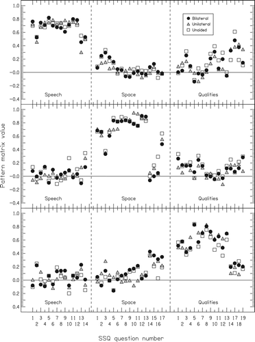
Speech questions #2, #13, and #14 are weighted noticeably lower than the others. Question #2 (“You are talking with one other person in a quiet, carpeted lounge-room. Can you follow what the other person says?”) is one of just two that refers to speech in quiet – all the rest refer to speech in some form of speech or noise background. Given that many people, even with a hearing loss, report little difficulty at speech in quiet it is therefore reasonable to find that this question differs from the others. We suggest that the reason why the other speech-in-quiet question (#3: “You are in a group of about five people, sitting round a table. It is an otherwise quiet place. You can see everyone else in the group. Can you follow the conversation?”) follows the main pattern is that it refers to a more-complex situation, one with five people in it (across all 1220 participants question #3 correlated at r = 0.63 and 0.68 with the two other questions about groups of five people, #4 and #6). The simplicity of situation may also account for why question #13 gives a relatively low loading (“Can you easily have a conversation on the telephone?”). We have no explanation of why question #14 should give a lower factor weighting than the others (“You are listening to someone on the telephone and someone next to you starts talking. Can you follow what’s being said by both speakers?”). It is not a particularly simple situation, and though it asks about the ability to follow both sources, so does #10 (“You are listening to someone talking to you, while at the same time trying to follow the news on TV. Can you follow what both people are saying?”).

The loadings for the Space questions generally cluster around zero. The slight gain around #2 and #3 might be due to their context being about locating people who are speaking (“You are sitting around a table or at a meeting with several people. You can”t see everyone. Can you tell where any person is as soon as they start speaking?” and “You are sitting in between two people. One of them starts to speak. Can you tell right away whether it is the person on your left or your right, without having to look?”).

Some of the loadings for the Qualities questions are substantially above zero. A few such questions are related to speech understanding: Question #3 mentions speaking (“You are in a room and there is music on the radio. Someone else in the room is talking. Can you hear the voice as something separate from the music?”), and question #17 is directly about speech (“When you are a passenger can you easily hear what the driver is saying sitting alongside you?”), though we are unsure as to why question #17 gave a substantially higher loading for the unaided group than for the aided groups. Two questions are indirectly related to being about speech, in that they concerned voices (#10 and #12: “Do other people”s voices sound clear and natural?”, and “Does your own voice sound natural to you?”). That questions #9, #14, #18, and #19 are about clarity, concentration, and effort suggests that listeners are relating them to speech when answering these (respectively, “Do everyday sounds that you can hear easily seem clear to you (not blurred)?”, “Do you have to concentrate very much when listening to someone or something?”, “Do you have to put in a lot of effort to hear what is being said in conversation with others?”, “Can you easily ignore other sounds when trying to listen to something?”). Note that questions #14 and #18 are of some interest as the loadings for the unaided group were somewhat lower than for the two aided groups—perhaps the explanation is that the unaided group do not relate these two questions on concentration and effort to speech understanding, but the aided groups do. The remaining questions mostly do not load on this factor. Two are recognition of person or mood by voice (#4 and #13). None of the others are concerned with situations that mention speech or voices.

F_SP = “Spatial Perception”

The middle panel of Figure 7 shows the weightings for F_SP. Again there is little difference between the results for the three groups. As the factor loads primarily on the Spatial questions, the factor is interpreted as being one of general spatial perception.

There are two clear sets of exceptions. The first is question #3 (“You are sitting in between two people. One of them starts to speak. Can you tell right away whether it is the person on your left or your right, without having to look?”). Given that this question gave a mean score that was at least 1.3 points higher than all the questions that did load strongly on this factor (7.5 vs. 4.9 to 6.2) we speculate that this question is considerably easier than the others and may not relate that well. The other exceptions are questions #14, #15, and #16 (respectively, “Do the sounds of things you are able to hear seem to be inside your head rather than out there in the world?”, “Do the sounds of people or things you hear, but cannot see at first, turn out to be closer than expected when you do see them?”, and “Do the sounds of people or things you hear, but cannot see at first, turn out to be further away than expected when you do see them?”). As noted above, these three questions gave particularly low communalities, where we noted that they deal with topics different to the remainder of the Space questions: #14 is concerned with the externalization or internalization of sounds, and questions #15 and #16 are concerned with how well perceived distance matches one's expectations. That question #17 (“Do you have the impression of sounds being exactly where you would expect them to be?”) gives a reasonably high weighting suggests that the effect is due to perceived distance rather than perceived location.

Occasional questions in the other sections gave loadings somewhat above zero on F_SP, at least for some of the participant groups (e.g. Speech #14, Qualities #1, #6, #19). There is no clear pattern to any of them.

F_CSI = “Clarity, Separation, and Identification”

The bottom panel of Figure 7 shows the weightings for F_CSI. The factor loads primarily on the Qualities questions, but in comparison to the other two factors the loadings are generally somewhat weaker and more variable across question. Given the diversity of questions in the Qualities section it is not obvious what to name the factor, but we feel that Clarity, Separation, and Identification is fair (we prefer to avoid Qualities by itself as that is properly reserved for the section as a whole).

The factor loads reasonably highly on the first 12 questions of the Qualities section. These are concerned with the separation of sounds in various forms, recognition of sounds, distinguishing sounds, and the clarity or naturalness of sounds. Four questions do not load on it. Questions #14, #18, and #19 are concerned with effort and concentration (respectively “Do you have to concentrate very much when listening to someone or something?”, “Do you have to put in a lot of effort to hear what is being said in conversation with others?”, “Can you easily ignore other sounds when trying to listen to something?”). That these three questions do not relate to the factor prevents us from incorporating “concentration/effort” into its name. Question #17 is an entirely separate topic (“When you are a passenger, can you easily hear what the driver is saying sitting alongside you?”). These four questions also all relate to F_SP and are discussed above.

For some patient groups there are respectable loadings for questions in the other two sections. Some of these (e.g. Speech #2, #13; Space #14, #15, #16) were remarked-on above as being exceptions to the general patterns for F_SU and F_SP. The interpretation is unclear.

General Discussion

We performed factor analyses of the SSQ responses from three groups of participants: unaided, unilaterally aided, and bilaterally aided. A parallel analysis demonstrated that three factors were clearly above chance. After oblique rotation, these three factors essentially matched the three sections of SSQ questions: one represented speech understanding, one represented spatial perception, and one represented clarity, separation, and identification. The analyses across the three groups were broadly similar. We therefore believe that the three-factor solution is reasonable. A potential fourth factor is discussed below.

The loading patterns of the three factors are particularly clear when plotted as the squares of the average factor weights across the three groups; i.e. the proportions of variance accounted for (see Figure 8). As there are no formal rules as to how high a proportion of variance is required to identify and separate factor loadings, we suggest a pragmatic and subjective summary based on visual inspection of Figure 8:

• All the speech questions except #2, #12, and #13 load on F_SU.

• All the spatial questions except #3, #14, #15, #16 and #17 load on F_SP.

• All of the qualities questions except #3, #14, #17, #18 and #19 load on F_CSI.

Figure 8. The squares of the average factor weights for each the 48 SSQ items. The symbols mark the three rotated factors. The weights are averaged across the three groups of listeners.

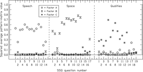
This gives a total of 35 questions that load on the three factors. The reader is reminded that Qualities #15 and #16 were removed from the analyses at an early stage due to a relatively high number of missing responses (see Methods).

The factor analysis has already proved useful in the development of the 12-question short form of the SSQ, the SSQ-12 (Noble et al, 2013). But it also indicates which questions do not go with the majority of the others. A potential application of this is to help guide the design of a future experiment should it be wished to add specific extra questions to the SSQ-12. For instance, the SSQ-12 includes three of the spatial questions (#6, #9, and #13). Given that all of these load on F_SP to about the same extent (see Figure 8), it would therefore be reasonable to add one of the questions that does not load on F_SP rather than another one that did.

Reliability of the factor loadings

We did not conduct formal statistical significance testing of the results for two reasons: (1) the data were not normally distributed, so the assumption of normality that underpins all parametric statistical tests was not valid, and (2) we were more concerned with the magnitude of the loadings rather than whether they were statistically significantly different from zero, as it is well known that even the tiniest difference can be made statistically significant if the sample size is large enough. Nevertheless, some estimate of the reliability of the factor loadings is necessary.

One approach is to do a random split-half analysis, but we did not do this because it halves the sample sizes and the results are somewhat dependent on the particular random halving used. Instead, we applied two separate methods. First, we performed a bootstrap analysis to obtain a measure of reliability (Efron & Tibshirani, 1994). For the unaided group, we randomly drew 386 sets of data, with replacement, from the n = 386 experimental datasets. The new dataset was then subject to a factor analysis, with three obliquely rotated factors, and the resulting loadings recorded. The process was repeated to give 50 sets of loadings, for which the distributions are calculated⁶. The standard deviation of this distribution is the bootstrap estimate of the standard error of the factor loadings, and so twice this value is an approximate 95% confidence interval for the factor loading (for illustrative applications of the bootstrap to factor analysis or its sister principal-components analysis, see Lambert et al, 1991; Efron & Tibshiran, 1994, p 61–80; Ichikawa & Konishi, 1995; Zientek & Thompson, 2007; Zhang et al, 2010)⁷. The process was repeated for the unilateral and bilateral groups. We found that the mean bootstrapped confidence interval on the weights was ± 0.14, averaged across all 432 confidence intervals (= 48 questions × 3 factors × 3 groups). A second measure of reliability can be found by noting that to some extent the three groups of participants effectively act as controls for each other. If the factor loadings are unreliable, then one would expect great differences across the groups. Instead, we found that the loadings from the three groups matched well: 97% of the possible differences between loadings were in the range ± 0.2 (97% = 419 of 432, where 432 = 48 questions ± 3 factors ± 3 pairwise differences). Visual inspection of the three sets of loadings (Figure 7) demonstrates that the patterns were similar across the groups. These results broadly support the bootstrap results. We therefore argue that the factor weights are generally accurate to within ± 0.1 to ± 0.2.

A potential fourth factor: Effort and Concentration

A preliminary analysis of the data that was reported earlier (Akeroyd et al, 2011) gave four factors. The primary differences in method between that analysis and the present one were that the earlier one used a smaller sample, namely 1105 datasets, and all the participants were included in one analysis, rather than separating them into three separate analyses by hearing aids. Three of the factors essentially corresponded to the three factors reported here. The fourth factor was given by an equal weighting of two items, qualities #14 and qualities #18 (respectively, “Do you have to put in a lot of effort to hear what is being said in conversation with others?”, “Can you easily ignore other sounds when trying to listen to something?”). It correlated at between − 0.4 and − 0.6 with the three main factors, at + 0.3 with hearing loss in the better ear, − 0.1 with the interaural asymmetry of hearing loss, at + 0.7 with the average SSQ score and + 0.6 with the average HHQ score. It is intriguing that items #14 and #18 were highlighted above as not loading on the main factor for the Qualities section, F_CSI (see Figures 7 and 8).

The present analyses used three factors because the parallel analysis demonstrated that the eigenvalues from only factors #1, #2, and #3 were found to be consistently above those of random data (see Figure 4). The eigenvalues of factors #5 and higher were clearly below the random data and therefore can be discounted. But the factor #4 was somewhat borderline. The eigenvalues of the observed data vs. the random data for the three groups of unaided, unilateral, and bilateral participants, respectively, were 1.38 vs. 1.57, 1.63 vs. 1.44, and 1.77 vs. 1.80. In only one of these was the observed above the random – though in the earlier analysis of 1105 people considered in one group, the corresponding values were 1.42 vs. 1.32. In the present analyses we deliberately applied the parallel-analysis criterion strictly in order to err on the side of caution. But equally we cannot rule out the fourth factor, and the experimenter who wishes to apply the parallel-analysis criterion more liberally may decide to include it.

Unitary-loaded factors

Some reviews of factor analysis note that there is often little loss of accuracy if, for all questions that load sufficiently on a factor to be included as part of it, every one is given the same loading of 1.0 instead of their actual individual loadings (e.g. Floyd & Widamen, 1995). For present purposes, this reduces to an equally-weighted average of the questions in each of the three sections after removing those questions that do not load on the factors:

The asterisks on F*_SU, F*_SP, and F*_CSI mark that unitary loadings are used instead of the actual factor loadings. It was found that the correlations between these equally-weighted scores and the properly-weighted factor scores were all at least 0.95. The differences are therefore small if the unitary-loaded scores F*_SU, F*_SP, and F*_CSI were to be used instead of the full factor scores. For reference, the corresponding equation for the fourth factor of Effort and Concentration is

Correlations with hearing loss

Table 4 reports the correlations between the equal-weighted scores F*_SU, F*_SP, and F*_CSI and various measures of hearing ability. It can be seen than in general the correlations: (1) with better-ear hearing loss were about − 0.2 to − 0.3, (2) with the interaural asymmetry of hearing level about − 0.1 to − 0.3, (3) with the unitary-weighted average of all 48 questions in the SSQ, SSQ₄₈—taken as a very simple overall measure of hearing disability—about + 0.8 to + 0.9, and (4) with the unitary-weighted average of all 12 questions in the hearing-handicap questionnaire (HHQ) were about − 0.5 to − 0.7. In the original SSQ paper Gatehouse and Noble (2004) reported a SSQ × hearing-loss correlation of − 0.5, and a SSQ × HHQ correlation of − 0.6. The present correlations therefore reproduce the ordering of these two, though there was a substantially lower correlation with hearing loss.

Table 4. Correlations of the equal-weighted scores (see equations 2–4) with various measures of hearing ability.

	F*SU	F*SU	F*SU	F*SP	F*SP	F*SP	F*CSI	F*CSI	F*CSI
	Unaided	Unilaterally	Bilaterally	Unaided	Unilaterally	Bilaterally	Unaided	Unilaterally	Bilaterally
Hearing level: BEA	− 0.37	− 0.20	− 0.23	− 0.33	− 0.27	− 0.32	− 0.36	− 0.28	− 0.36
Hearing level: asymmetry	− 0.21	− 0.12	− 0.14	− 0.33	− 0.30	− 0.17	− 0.08	− 0.13	− 0.12
Hearing disability: SSQ48	+ 0.87	+ 0.83	+ 0.85	+ 0.90	+ 0.89	+ 0.90	+ 0.86	+ 0.88	+ 0.91
Hearing handicap: HHQ12	− 0.70	− 0.52	− 0.53	− 0.58	− 0.52	− 0.51	− 0.57	− 0.54	− 0.60

Other divisions of the participants

The above analyses are based on dividing the 1220 participants into three broad groups of unaided, unilaterally aided, and bilaterally aided. We felt that two other divisions would be of interest, and so we repeated the analyses.

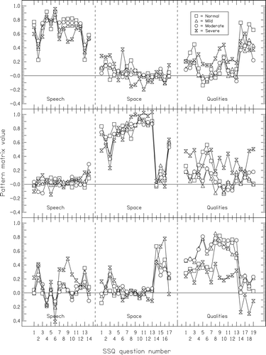
First, we divided the listeners by hearing loss, into groups of normal hearing, mild loss, moderate loss, and severe loss (defined, respectively, by criteria of < 20 dB; 20–40 dB; 41–70 dB, and 71–95 dB; N = 214, 439, 477, 74) (British Society of Audiology, 2011). The factor analyses within each group were done using the same method as before, except that we forced it to give three factors instead of doing a parallel analysis. Figure 9 shows the results. It can be seen that the results were similar to those obtained above: the pattern of weights across question shown in Figure 9 is comparable to that shown in Figure 7. The only noteworthy difference is that the pattern on the Qualities questions for the Severe group (double triangles), in comparison to the other groups, is one of higher weights on the second factor (middle row) and correspondingly lower weights for the third factor (bottom) row. That is, their reports can be fairly summarized by two main factors, on Speech and Space, but Qualities plays less of an independent role. This intriguing result needs confirmation by further work.

Figure 9. As Figure 7 but for the participants divided by hearing loss. The four groups were normal hearing, mild loss, moderate loss, and severe loss, with criteria of < 20 dB; 20–40 dB; 41–70 dB, and 71–95 dB (N = 214, 439, 477, 74 respectively).

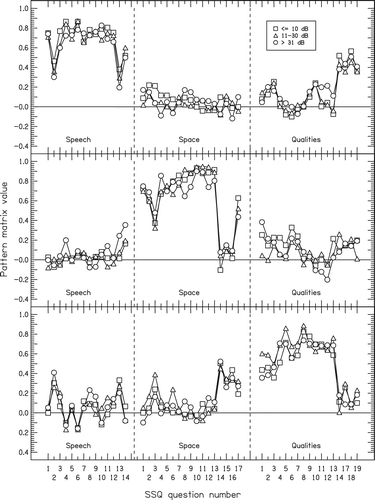
Second, we divided the listeners by interaural asymmetry, with criteria of ≤ 10 dB, 11–30 dB, and > 31 dB (for essentially symmetric, partly asymmetric, and highly asymmetric; n = 739, 316, 165 respectively). Figure 10 shows the results. The weights closely correspond to those shown in Figure 7, and there were no substantial differences across groups. Note that the highly asymmetric group did not give a different pattern to the other groups on the Spatial questions.

Figure 10. As Figure 7 but for the participants divided by interaural asymmetry. The three groups were defined by criteria of ≤ 10 dB, 11–30 dB, and > 31 dB, for essentially symmetric, partly asymmetric, and highly asymmetric (n = 739, 316, 165 respectively).

Comparisons to the spatial hearing questionnaire

Tyler et al's (2009) Spatial Hearing Questionnaire has 24-questions that inquire about understanding speech in various situations (9 questions), hearing music clearly (3), location of various sounds in various situations (10), movement (1), and distance (1). Tyler et al reported a principal-components analysis of data from 142 cochlear-implanted listeners, with the criterion of eigenvalues > 1 then varimax rotation and a total variance explained of 65%. They found three overall factors, the first, “directionality”, representing all 12 of the location, movement, and distance questions, a second representing most (nine) of the speech-understanding and hearing-music questions and interpreted as being the more-difficult situations, and the third representing the remainder (three) of the speech and music questions, concerned with easier situations. The three factors correlated at 0.8, 0.7, and 0.6, respectively with the listeners’ average score on the whole SSQ, and at 0.8, 0.6, and 0.5 with the average score on the Speech section. It is encouraging that Tyler et al's analysis gave a broad spatial factor that included, and included fairly equally too in weight, a large number of localization questions (their reported weights were all between 0.76 and 0.91). Our result was similar: many of the SSQ's spatial questions weight about the same on the Spatial Perception factor. Moreover, the various SSQ questions that do not appear in that factor are to do with internalization of sounds (#14), one's expectations of where a sound will be (#15, #16, #17), and a simple left-right discrimination (#3)—these domains are not inquired in Tyler et al's spatial hearing questionnaire. We also note that the two SSQ Speech questions that deal with very Simple listening situations (#3, listening to one person in quiet, and #13, conversation on the telephone) were not included in the Speech Understanding factor. This parallels Tyler et al's separation of more-difficult speech situations from easier.

Summary

We performed an oblique-rotation factor analysis of the SSQ responses from 1220 participants, split into three groups of participants of unaided, unilaterally aided, and bilaterally aided. We found three clear factors, essentially corresponding to the three main sections of the SSQ, and termed “speech understanding”, “spatial perception”, and “clarity, separation, and identification”. The analyses across the three groups were broadly similar. There was partial evidence for a fourth factor, “effort and concentration”. Thirty-five of the questions were included (37 if the fourth factor is included). It is suggested that the unitary-loaded scores (see Equations 2, 3, and 4) rather than the full factor scores will be sufficiently accurate for most purposes.

Acknowledgements

We thank the staff of the Scottish Section for collecting the data over the past 10 years, Graham Naylor (Eriksholm) & Oliver Zobay (IHR) for comments on the manuscript, Kelly Demeester (Leuven) for her cluster-analysis data, and the editors and reviewers of IJA for their informative comments during submission. Earlier versions of the analysis were presented at the 2011 ICRA meeting and the 2011 British Society of Audiology Annual Conference.

Declaration of interest: The authors report no declarations of interest. This work was supported by the Medical Research Council (grant number U135097131) and by the Chief Scientist Office of the Scottish Government.

Notes

Notes

1. Gatehouse and Noble (2004) list 50 items. One item, however, asks specifically about the effect of hearing aids or cochlear implants (Qualities #15). It is therefore excluded from many studies that are concerned with unaided listening.

2. We encourage users of the SSQ to ensure that all questions are answered.

3. The 49 questions used by Noble et al (2013) are the 48 questions considered here, plus Qualities #17.

4. This description of the dependence of SSQ scores on hearing loss, etc. is deliberately limited, as the present paper concentrates on the factor analysis itself. We hope to publish other analyses in the future.

5. As we earlier excluded those people who did not fully complete the SSQ, none of these matrices had any missing observations.

6. Occasionally we came across what is known as the alignment problem: the factors were reported in a different order or with negative weights instead of positive (Zhang et al, 2010). We silently corrected all of these by hand.

7. Many bootstrap applications use thousands of replications in order to obtain very accurate confidence intervals, but Efron and Tibshirani (1994, p. 52) suggested that 50 replications was often enough to get a good estimate of the standard error. Also we did not apply either the bias or acceleration corrections, mainly to simplify the calculations (Efron & Tibshirani, 1994; see Zhang et al, 2010 for their effects in bootstrapped factor analyses). Thus our estimates of the confidence intervals can only be estimates, but we contend that they are sufficiently accurate for present purposes.

References

- Ahlstrom J.B., Horwitz A.R. & Dubno J.R. 2009. Spatial benefit of bilateral hearing aids. Ear Hear, 30, 203–218.
- Akeroyd M.A. & Guy. F.H. 2011. The effect of hearing impairment on localization dominance for single-word stimuli. J Acoust Soc Am, 130, 312–323.
- Akeroyd M.A., Guy F.H., Harrison D.L. & Suller S.L. 2011. A factor analysis of the Speech, Spatial and Qualities of Hearing Questionnaire (SSQ). Int J Audiol, 51, 262 (conference abstract).
- Banh J., Singh G. & Pichora-Fuller M.K. 2012. Age affects responses on the Speech, Spatial, and Qualities of Hearing Scale (SSQ) by adults with minimal audiometric loss. J Am Acad Audiol, 23, 81–91.
- British Society of Audiology. 2011. Recommended procedure: Pure-tone air-conduction and bone-conduction threshold audiometry with and without masking. Reading: British Society of Audiology.
- Browne M.W. 2001. An overview of analytic rotation in exploratory factor analysis. Multivariate Behavioural Research, 36, 111–150.
- Carroll J.B. 1993. Human Cognitive Abilities: A Survey of Factor-analytic Studies. Cambridge: CUP.
- Cattell R.B. 1966. The Scree test for the number of factors. Multivariate Behavioral Research, 1, 245–276.
- Cattell R.B. & Vogelmann S. 1977. A comprehensive trial of the Scree and KG criteria for determining the number of factors. Journal of Multivariate Behavioral Research, 12, 289–325.
- Comrey A.L. & Lee H.B. 1992. A First Course in Factor Analysis. Hillsdale, USA: Lawrence Erlbaum Associates.
- Costello A.B. & Osborne J.W. 2005. Best practices in exploratory factor analysis: Four recommendations for getting the most from your analysis. Practical Assessment, Research and Evaluation, 10, 173–178.
- Cudeck R. & MacCallum R.C. (eds.). 2007. Factor Analysis at 100: Historical Developments and Future Directions. Mahweh, USA: Lawrence Erlbaum Associates.
- Demeester K., Topsakal V., Hendrickx J.J., Fransen E., van Laer L. et al. 2012. Hearing disability measured by the Speech, Spatial, and Qualities of Hearing Scale in clinically normal-hearing and hearing-impaired middle-aged persons, and disability screening by means of a reduced SSQ (the SSQ5). Ear Hear, 33.
- Dinno A. 2009. Exploring the sensitivity of Horn”s parallel analysis to the distributional form of random data. Multivariate Behavioral Research, 44, 362–388.
- Douglas S.A., Young P., Daudia A., Gatehouse S & O’Donoghue G.M. 2007. Spatial hearing disability after acoustic neuroma removal. Laryngoscope, 117, 1648–1651.
- Efron B & Tibshirani R.J. 1994. An Introduction to the Bootstrap. Boca Raton, Florida: Chapman & Hall/CRC.
- Fabriger L.R., Wegener D.T., MacCallum R.C. & Strahan E.J. 1999. Evaluating the use of exploratory factor analysis in psychological research. Psych Methods, 4, 272–299.
- Field A. 2009. Discovering Statistics using SPSS. London: Sage.
- Floyd F.J. & Widaman K.F. 1995. Factor analysis in the development and refinement of clinical assessment instruments. Psych Assessment, 7, 286–299.
- Galvin K.L., Hughes K.C. & Mok M. 2010. Can adolescents and young adults with prelingual hearing loss benefit from a second, sequential cochlear implant?Int J Audiol, 49, 368–377.
- Galvin K.L., Mok M. & Dowell R.C. 2007. Perceptual benefit and functional outcomes for children using sequential bilateral cochlear implants. Ear Hear, 28, 470–482.
- Gatehouse S. & Akeroyd M.A. 2006. Two-eared listening in dynamic situations. Int J Audiol, 45 (Suppl. 1), S120–S124.
- Gatehouse S. & Noble W. 2004. The Speech, Spatial and Qualities of Hearing Scale (SSQ). Int J Audiol, 43, 85–99.
- Guadagnoli E. & Velicer W.F. 1988. Relation of sample size to the stability of component patterns. Psychol Bull, 103, 265–75.
- Hayton J.C., Allen D.G. & Scarpello V. 2004. Factor retention decisions in exploratory factor analysis: A tutorial on parallel analysis. Organizational Research Methods, 7, 191–205.
- Helfer K.S & Vargo M. 2009. Speech recognition and temporal processing in middle-aged women. J Am Acad Audiol, 20, 264–271.
- Horn J.L. 1965. A rationale and test for the number of factors in factor analysis. Psychometrika, 30, 179–185.
- Jensen N.S., Akeroyd M.A., Noble W. & Naylor G. 2009. The Speech, Spatial and Qualities of Hearing scale (SSQ) as a benefit measure. Poster presented at the NCRAR conference on “The Ear-Brain System: Approaches to the Study and Treatment of Hearing Loss”, Portland, October 2009 (see http://www.ihr.mrc.ac.uk/products/display/ssq).
- Jennrich R.I. 1979. Admissible values of gamma in direct oblimin rotation. Psychometrika, 44, 173–177.
- Jennrich R.I. 2007. Rotation methods, algorithms, and standard errors. In: Cudeck & MacCallum (eds.). Factor Analysis at 100: Historical Developments and Future Directions. Mahweh, USA: Lawrence Erlbaum Associates, pp. 315–336.
- Kaiser H.F. 1960. The application of electronic computers to factor analysis. Educational and Psychological Measurement, 20, 141–151.
- Kaiser H.F. 1970. A second generation little jiffy. Psychometrika, 35, 401–415.
- Kass R.A. & Tinsley H.E.A. 1979. Factor analysis. Journal of Leisure Research, 11, 120–138.
- Keidser G., O’Brien A., Hain J.U., McLelland M. & Yeend I. 2009. The effect of frequency-dependent microphone directionality on horizontal localization performance in hearing-aid users. Int J Audiol, 48, 789–803.
- Kiessling J., Grugel L., Meister H. & Meis M. 2011. Übertragung der fragebögen SADL, ECHO und SSQ ins Deutsche und deren Evaluation [German translations of questionnaires SADl, ECHO, and SSQ and their evaluation]. Z Audio, 50, 616.
- Kobler S., Lindblad A.C., Olofsson A. & Hagerman B. 2010. Successful and unsuccessful users of bilateral amplification: Differences and similarities in binaural performance. Int J Audiol, 49, 613–627.
- Ichikawa M. & Konishi S. 1995. Application of bootstrap methods in factor analysis. Psychometrika, 60, 77–93.
- Lambert Z.V., Wildt A.R. & Durand R.M. 1991. Approximating confidence intervals for factor loadings. Multivariate Behavioral Research, 26, 421–434.
- MacCallum R.C., Widaman K.F., Zhang S. & Hong S. 1999. Sample size in factor analysis. Psych Methods, 4, 84–99.
- Martin T.P.C., Lowther R., Cooper H., Holder R.L., Irving R.M. et al. 2010. The bone-anchored hearing aid in the rehabilitation of single-sided deafness: Experience with 58 patients. Clin Otolaryngol, 35, 284–290.
- Most T., Adi-Bensaid L., Shpak T., Sharkiya S. & Luntz M. 2012. Everyday hearing functioning in unilateral versus bilateral hearing-aid users. American Journal of Otolaryngology – Head & Neck Medicine and Surgery, 33, 205–211.
- Noble W. & Gatehouse S. 2004. Interaural asymmetry of hearing loss, speech, spatial, and qualities of hearing scale (SSQ) disabilities, and handicap. Int J Audiol, 43, 100–114.
- Noble W. & Gatehouse S. 2006. Effects of bilateral versus unilateral hearing aid fitting on abilities measured by the speech, spatial, and qualities of hearing scale (SSQ). Int J Audiol, 45, 172–181.
- Noble W., Tyler R., Dunn C. & Bhullar N. 2008. Unilateral and bilateral cochlear implants and the implant-plus-hearing-aid profile: Comparing self-assessed and measured abilities. Int J Audiol, 47, 505–514.
- Noble W., Naylor G., Bhullar N. & Akeroyd M.A. 2012. Self-assessed hearing abilities in middle- and older-age adults: A stratified sampling approach. Int J Audiol, 51, 174–180.
- Noble W., Jensen N.S., Naylor G., Bhullar N. & Akeroyd M.A. 2013. A short form of the speech, spatial, and qualities of hearing scale suitable for clinical use: The SSQ12. Int J Audiol, 52, 409–412.
- Odelius J. & Johansson O. 2010. Self-assessment of classroom assistive listening devices. Int J Audiol, 49, 508–517.
- Pohlmann J.T. 2004. Use and interpretation of factor analysis in the Journal of Educational Research: 1992–2002. Journal of Educational Research, 98, 14–22.
- Potts L.G., Skinner M.W., Litovsky R.A., Strube M.J. & Kuk F. 2009. Recognition and localization of speech by adult cochlear implant recipients wearing a digital hearing aid in the non-implanted ear (bimodal hearing). J Am Acad Audiol, 20, 353–373.
- Preacher K.J. & MacCullum R.C. 2003. Repairing Tom Swift's electric factor analysis machine. Understanding Statistics, 2, 13–43.
- Singh G. & Pichora-Fuller M.K. 2010. Older adults’ performance on the speech, spatial, and qualities of hearing scale (SSQ): Test-retest reliability and a comparison of interview and self-administration methods. Int J Audiol, 49, 733–740.
- Spearman C. 1904. ‘General Intelligence’, objectively determined and measured. Am J Psych, 15, 201–292.
- Stevens J. 1996. Applied Multivariate Statistics for the Social Sciences. Mahwah, USA: Lawrence Erlbaum Associates.
- Tabachnick B.G. & Fidell L.S. 2007. Using Multivariate Statistics. Boston: Pearson.
- Thompson B. & Daniel L.G. 1996. Factor analytic evidence for the construct validity of scores: A historical overview and some guidelines. Educational and Psychological Measurement, 56, 197–208.
- Thurstone L.L. 1935. The Vectors of Mind. Chicago: University of Chicago Press.
- Tyler R.S., Perreau A.E. & Haihong J. 2009. Validation of the Spatial Hearing Questionnaire. Ear Hear, 30, 466–474.
- van Wieringen A., de Voecht K., Bosman A.J. & Wouters J. 2011. Functional benefit of the bone-anchored hearing aid with different auditory profiles: Objective and subjective measures. Clin Otolaryngol, 36, 114–120.
- Velicer W.F. & Jackson D.N. 1990. Component analysis versus common factor analysis: Some issues in selecting an appropriate procedure. Multivariate Behavioral Research, 25, 1–28.
- Zientek L.R. & Thompson B. 2007. Applying the bootstrap to the multivariate case: Bootstrap component/factor analysis, Behavior Research Methods, 39, 318–325.
- Zhang G., Preacher K.J. & Luo S. 2010. Bootstrap confidence intervals for ordinary least squares factor loadings and correlations in exploratory factor analysis. Multivariate Behavioral Research, 45, 104–134.
- Zwick W.R. & Velicer W.F. 1986. Comparison of five rules for determining the number of components to retain. Psych Bull, 99, 432–442.