Failure criterion for timber beams loaded in bending, compression and shear

Introduction

In the 1970s, strength tests at the Delft Stevin laboratory for combined bending and compression demonstrated a volume effect leading to a follow-up programme on semi-full-scale glulam beams with the theoretically necessary perfect boundary conditions of the supports. Damage always occurred through lateral buckling following cracking sounds during loading and a decrease in the modulus of elasticity after unloading, even when the test was stopped at the smallest possible lateral displacements. This applies even for the most slender beams, applied in praxis, which were expected to remain elastic, suitable for further testing of multiload combinations. The theory of elasticity in Chen and Atsuta (1972) does not show bifurcation for the three-dimensional lateral buckling case, and the large displacements analysis (third order theory) shows a continuous rise in the loading curve. This means that the top of a loading curve always is due to damage and failure and therefore elastic buckling does not exist in praxis for structural elements. Stability design is a common second order strength calculation. The solutions of the second order equilibrium equations have to satisfy the failure criterion. This failure criterion is therefore essential and has to be discussed first. As shown in van der Put (Citation2009), for statically indeterminate structures, and here, for combined loading, in wood design the idealized linear elastic calculation applied for failure, as given by the dashed lines in Figure 1, is not sufficient to describe and predict strength behaviour and needs to be replaced by the elastic–plastic calculation (solid lines in Figure 1). The existing models and proposed design rules of the Eurocode 5 (2004) therefore have to be corrected in this way. At the moment three different criteria are prescribed in the Eurocode for basically the same strength calculation: n ²+m=1 (eq. 6.19), n+m=1 (eq. 6.23) and m ²+n=1 (eq. 6.35), where n and m are the normalized real compression and bending loadings N/N _u and M/M _u relative to the ultimate compression strength N _u and bending strength M _u.

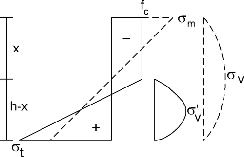
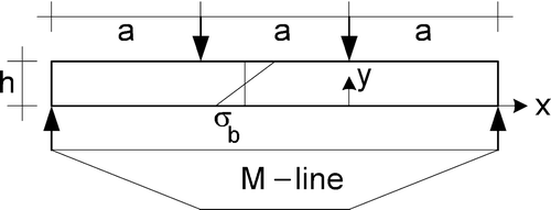
Figure 1.  Bending and shear stress.

Display full size

This needs to be replaced by one equation of the real failure criterion (eq. Equation5), which accounts for the elastic–plastic behaviour of wood, showing unlimited plastic flow in compression and brittle-like behaviour in tension (thus showing a volume effect for tension). The hypothesis of limited ultimate strain in compression followed so far is too conservative and has to be abandoned. Finite ultimate strain is not a material property but is caused by instability of the test. Limited strain was introduced for concrete in the 1960s by the parabolic stress diagram. It appeared that this diagram had to be extended by a full plastic range to be able to describe combined bending–compression failures. The same applies for steel and wood. The previous models for wood (e.g. Johns & Buchanan, Citation1982; Blass, Citation1987) are based on the principle of limited flow, leading to inconsistent adaptations that have to be corrected, especially because the Eurocode and other standards are based on this invalid restriction.

Derivation of the failure criterion for bending with compression and shear

The idealized elastic–plastic bending strength behaviour of wood (Figure 1), based on plasticity theory, provides the highest lower bound of the strength of limit analysis. The description is therefore the closest to the exact solution and close to the actual behaviour and measurements, and thus is able to predict behaviour. The equilibrium equations of this beam with width b and height h, loaded by a moment M, normal force N and shear force V are, according to Figure 1:

According to Figure 1, the shear force V for failure is, when and thus when the apparent linearized elastic shear stress σ _v=f _v:

For N=0, the shear strength is V _u=V _u,0 and eq. (Equation8) can be written:

Parameter estimation

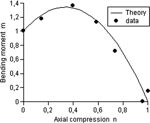
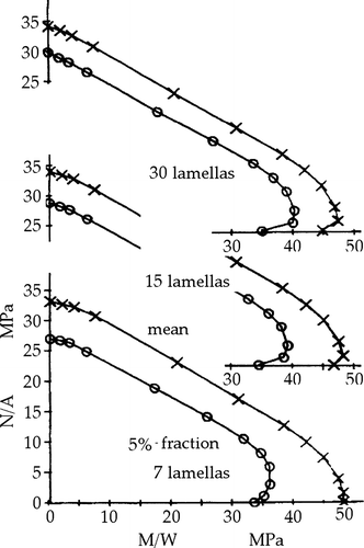
As for the discussed models, the data of Johns and Buchanan (Citation1982) are used here for parameter estimation of eq. (Equation5). Each point of Figures 2–5 represents test results of 100 boards of 89×140 mm lumber of the spruce–pine–fir species group of grade 2 and better, kiln dried. The data are given in Figure 2. Because the nominal scale is not right, only normalized quantities are used. Equation (Equation5) will be written:

Figure 2.  Combined bending–compression and bending–tension strength.

Display full size

Figure 3.  s=2 or 95th percentile of the bending–compression strength.

Display full size

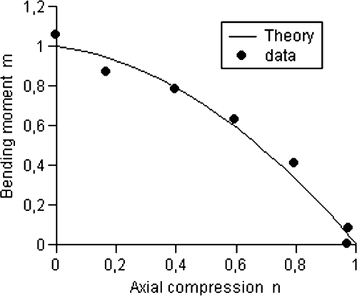
Figure 4.  s=1.3 or 50th percentile of the bending–compression strength.

Display full size

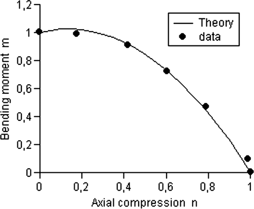
Figure 5.  s=0.77 or 5th percentile of the bending–compression strength.

Display full size

Trials show that:

• for the 95th percentile, s=2 and eq. (Equation11) becomes m=1−0.2n−0.8n ²

• for the 50th percentile, s=1.3 and eq. (Equation11) becomes m=1+0.38n−1.38n ²

• for the 5th percentile, s=0.77 and eq. (Equation11) becomes m=1+2.05n−3.05n ².

A higher value than s=1.3 is necessary to fit the data for combined bending with tension. The sketched mean strength line of Figure 2, the parabolic failure criterion of the Eurocode 5, shows a maximum of m of eq. (Equation11) at n=0. Thus:

Because the specimen compression strength f _c and pure tensile strength f _t,p (Figure 2) are also measured, the volume effect is directly known. For the 50th percentile it is:

Figure 6.  Interaction curve cut-off (by the dashed shear line) or no cut-off (by the drawn ultimate shear line).

Display full size

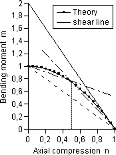
Shear failure mechanisms are discussed in van der Put (Citation2009). The shear strength V _u here is:

For average wood qualities, the shear slenderness is 3 for failure in shear at the maximum possible bending strength. It then follows from eq. (Equation9) that for a/h=3:

Bending curvature

The relation for the radius of bending R follows from the maximal elastic stresses of Figure 1. Using eq. (Equation2) with N=0 and eq. (Equation4) the curvature is:

To eliminate the varying values of s along the beam, this can be approximated to:

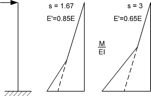
Thus, the apparent linear elastic modulus of elasticity E′ follows from a reduced modulus by plastic deformation (Figure 7). When the normal force is not zero, the derived curvature becomes:

Figure 7.  Estimation of the reduced modulus of elasticity.

Display full size

Correction of previous approximations

Johns and Buchanan (Citation1982) explained their data of Figure 2 by elastic tension and elastic–plastic compression behaviour. However, a finite ultimate flow strain in compression is assumed to exist and the behaviour therefore remains partly close to elastic, but may also lead to inconsistencies. For instance, when a column fails in pure compression reaching ultimate strain, then rotation of the cross-section is possible, increasing the external moment by the eccentricity of the compression load, while the stress remains fully plastic and the internal moment remains zero. Thus, equilibrium for this assumed failure state is not possible. When a beam fails in pure bending, reaching the ultimate compression strain, then any additional axial loading will decrease the bending tension stress, which remains elastic, and the parameter s=σ _t/f _c becomes dependent on the loading and an arbitrary choice of s becomes possible for combined loading. This is demonstrated by the limit flow assumption of Blass (Citation1987). In this model, not the mean ultimate stress, but the maximum stress, before the very small yield drop at the start of flow (Figure 8), is chosen as ultimate bending compression stress, limiting the ultimate strain up to this point. Besides the very low ultimate strain, the ultimate stress value is questionable because yield drop is not a material property (van der Put, Citation1989 ,Citation2007), but depends on the rate of loading, temperature, etc., and on the total specimen–testing machine stiffness. It only occurs in a constant strain rate test and thus not in a constant loading rate test or at dead load failure in practice. Further, the moment–curvature diagrams of the model (Figure 8) (of Blass Citation1987) are also questionable because of the following: (1) A constant ultimate moment cannot exist at an increasing curvature at flow when the normal force (n=0.7) is constant because of the increase in the external moment. (This may only apply for virtual displacements). (2) A decrease in the bending moment at the increase of the curvature is not possible because for a constant loading N, the external moment increases with the increase in deformation and eccentricity, e. Thus, the decrease by yield drop and stepwise decrease in stress at high curvatures in Figure 8 are not possible in a real test (or real simulation) of an eccentric loaded column.

Figure 8.  Fictive curvature diagrams (Blass, Citation1987).

Display full size

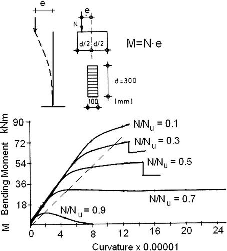
However, the diagrams serve a useful purpose to show the model assumptions made by Blass (Citation1987) for the strength calculation. The dashed line in Figure 8 intersects the chosen ultimate stress points (at the start of the yield drop) for the different values of N, showing that a (non-linear) elastic calculation of the strength is applied that is linearized by the applied secant modulus, where M/(1−N/N _u) is constant. Extrapolated to pure bending strength M _u,0 (N=0), the found ultimate load criterion becomes M/(1−N/N _u)=M _u,0 or , equal to eq. (Equation6). This quasi-elastic solution, based on the start of initial flow, is questionable for real plastic behaviour because it wrongly is based on the linear proportionality of the curvature with the bending stress σ _m, while eq. (Equation21) shows this to be quadratically proportional with . The quasi-elastic equation found by Blass (eq. Equation6) is therefore far below the strength data and is modified to:

Figure 9.  Fictive interaction lines (Blass, Citation1987).

Display full size

The empirical eq. (Equation23) can be explained by the theory (eq. Equation5), leading to , showing that in the Blass model 3s−1 is chosen to be proportional to n as an arbitrary loading-dependent ultimate tensile stress condition.

For the pure compression strengths, at the compression axis, a volume effect is suggested to exist, giving in Figure 9 the curved deviations from the straight line near the compression axis of the seven-, 15- and 30-laminate beams. Partly this is due to the change from bending failure to pure compression failure (changing s quickly), but probably is mainly due to following the curve of Johns and Buchanan (Citation1982). This apparent volume effect is explained as follows. The tests of Johns and Buchanan (Citation1982) were performed on two different pieces of test equipment, one for pure compression and the other for combined bending–compression. This caused a small difference between the measured pure compression strength and the extrapolated compression strength from the combined bending–compression test data. This also explains why this assumed (non-existent) volume effect is in the wrong direction.

The departure of Blass (Citation1987) from the straight model line at lower normal loading also follows the fit of Johns and Buchanan (Citation1982) for the seven-laminate beams, suggesting that now the bending–compression strength is no longer regarded as being determining for failure, but rather the bending tensile stress, with f _m=48 MPa instead of the assumed 60 MPa of the straight line of the finite ultimate compression strain model. According to the theory, this leads to , or s=1.45.

However, the value of s is not constant along the curve of Blass and thus does not follow Johns and Buchanan's fit of the data (with s=1.3), but follows their sketched parabolic line, leading to a maximum bending strength at N=0 and thus to the incorrect value of s=1.67 for this failure criterion, which is introduced in the Eurocode. The same applies, for example, for the beam with 30 laminations. This combined compression–bending strength curve is also not based on an ultimate bending tension strength calculation because s never is constant along the curve and is about 1.55 at the top of the curve, reducing to below a value of s=1 when N=0, indicating a very low tensile strength (in disagreement with the applied regression equations). The contrary is to be expected for laminated wood and the real curves therefore can be expected to be flat, like the one in Figure 3.

Because the probability functions of the regression equation, applied by Blass, do not contain a volume parameter and therefore his model cannot account for a size effect, estimation of this effect is necessary. For comparison, the mean tensile strength of the standard laminate is given to be 55.4 MPa, but without specifying dimensions and length belonging to this strength.

The tensile strengths of the simulation model beams with the different bending strength values of about 48, 46.5 and 45 MPa (of Figure 9) can be verified as follows. According to Figure 9, for the beams with seven, 15 and 30 laminations, the coefficient of variation is v ₇=(48−34)/(1.64 · 48)=0.178. Thus, 1/k=0.3 · 0.178=0.0534. The coefficient of variation is v ₁₅=(46.5−35)/(1.64 · 46.5)=0.151. Thus, 1/k=0.3 · 0.15=0.045. The coefficient of variation is v ₃₀=(45−35)/(1.64 · 45)=0.136. Thus, 1/k=0.3 · 0.136=0.0408. The factor 0.3 follows from the volume effect as follows. Because the bending strength follows from the beam dimension L/h=18, at the same width b, the volume ratio is and the strength of the 15-laminate beam with respect to the seven-laminate beam is , giving 2α=0.0417/0.151≈0.3. The same rounded value of α follows from the strength of the 30-laminate beam with respect to the seven-lamella beam according to . This value of α of 0.15 is too low, far below the values found empirically (see Appendix). This leads to the pure tensile strength of the beams with seven, 15 and 30 laminations, respectively, according to eq. (Equationa7) of:

The value of 2α=1.0 (van der Put, Citation1977) leads, as a first approximation, to more probable bending strengths with respect to the value of 48 MPa of the seven-laminate beams of MPa for the 15-laminate beam and MPa for the 30-laminate beam (applying for stable tests).

Conclusions

The assumption of the existing models for combined bending and compression loading, (discussed in the previous section) that a specific compression strain limit is determining for failure is shown to be incorrect. For instance, it predicts from the compression failure that there is no size effect of the strength. The measurements and theory show that there always is a size effect at any value of s and for any load combination because the bending tensile strength is always greater than the pure tension strength of the specimen. For this reason, bending tension failure always occurs, which leads to the starting point of unlimited flow in compression of the plasticity approach modified here.

The derived failure criterion for combined bending with compression is given by eq. (Equation5). This equation can be approximated to two straight lines (eqs Equation15 and Equation16), providing simple equations for design and for implementation of the Code.

The derived failure criterion for combined shear with bending and compression is given by eq. (Equation9). Because this line will give a cut-off of the ultimate bending–compression strength lines, this combined shear strength criterion always has to be checked, which should be in the Code.

The size effect is lacking throughout the Blass model, giving questionable predictions of the strengths and an incorrect form of the interaction curves. The parabolic failure criterion of the Johns and Buchanan and Blass models, applied for Eurocode 5, is unsafe and denies the strong influence of quality and moisture content on the form of the curve (given by the parameter s).

The derived equation (eq. Equation21) shows the curvature along the beam to be a quadratic function of the bending stress σ _m, instead of a linear function of σ _m, as is the incorrect basis of the existing approaches discussed in the previous section. Equation (Equation21) provides a simple method for the ultimate deformation calculation and thus for the ultimate second order bending moment estimation.

References

- Blass , H. J. 1987 . Tragfähigkeit von Druckstäben aus Brettschichtholz unter berücksichtigung streuender Einflussgrössen . Thesis, University of Karlsruhe. (See also CIB-W18/19-12-2 and CIB-W18/20-2-2.)
- Chen , W. F. and Atsuta , T . 1977 . Theory of beam-columns. Vol.2: Space behaviour and design , New York : McGraw-Hill .
- Eurocode 5 2004 . EN 1995-1-1 Design of timber structures, Part 1-1: General—Common rules and rules for buildings . Technical committee CEN/TC50 Structural Eurocode, Secretariat BSI .
- Johns , K. C. Buchanan , A. H. 1982 . Strength of timber members in combined bending and axial loading . CIB/IUFRO Meeting , Boras , Sweden . (See also CIB-W18, 1985, Israel.)
- van der Put , T. A. C. M. 1977 . Influence of specimen dimensions on strength properties of glulam (Rep. 4-77-5 he-7) . Delft : Stevin Laboratory, Delft University . (In Dutch.)
- van der Put , T. A. C. M. 1981 . Finger-joints in glulam (Rep. 4-81-5 VL-3) . Delft : Stevin Laboratory, Delft University . (In Dutch.)
- van der Put , T. A. C. M. 1989 . Deformation and damage processes in wood . Delft : Delft University Press .
- van der Put , T. A. C. M. 1990 . Stability design and code rules for straight timber beams . Meeting CIB-W18/23-15-2 .
- van der Put , T. A. C. M. 2007 . Softening behaviour and correction of the fracture energy . Theoretical and Applied Fracture Mechanics , 48 : 127 – 139 .
- van der Put , T. A. C. M. 2009 . Derivation of the shear strength of continuous beams . Holz als Roh Werkst (accepted) .
Appendix: Size effect
The influence of the size effect always has to be regarded in strength calculations. For the general applicability a simple derivation of the size effect is given in the following.
The survival probability of a specimen with volume V, loaded by a constant tensile stress σ, as in the standard tensile test, can be given as function of the stress by:
For a stress distribution eq. (Equationa1) becomes:
For the stress distribution, , according to , is:
Figure 10. Four-point bending test.
According to eqs (Equationa3) and (Equationa6), the bending strength of the bending tests is:
The 900 mm specimens of the compression–bending tests were loaded by eccentrical compression and thus by a constant moment along the length. According to eqs (Equationa3) and (Equationa5) the bending strength (for zero compression) is:
In the derivation above the linearized bending strength is used. This is possible because the triangle tensile stress area of the real elastic–plastic stress distribution in is about equal to that of the linear stress distribution (the dashed line in ). This is verified by tests of van der Put (Citation1981), where in this way f m/f t,p ≈ 1.27 was predicted and measured in the four-point bending test, while f m/f t,p ≈ 2.3 was predicted and 2.2 was measured in the three-point bending test.
The discussion of the volume effect for combined bending with tension is not discussed in this article. For low tension, the equations are the same as for compression, with an opposite sign for the uniform tensile stress. For high tension the calculation is according to the theory of elasticity as discussed by Johns and Buchanan (Citation1982).
The Weibull constant k for brittle failure is given by eq. (Equationa9):