
 ?Mathematical formulae have been encoded as MathML and are displayed in this HTML version using MathJax in order to improve their display. Uncheck the box to turn MathJax off. This feature requires Javascript. Click on a formula to zoom.
Abstract
A graph with edges is called
if its edges can be labeled with 1, 2,
,
such that the sums of the labels on the edges incident to each vertex are distinct. Hartsfield and Ringel conjectured that every connected graph other than
is antimagic. In this paper, through a labeling method and a modification on this labeling, we obtained that the lexicographic product graphs
are antimagic.
Keywords:
1 Introduction
Graphs considered here are all simple, connected, finite and undirected. A path with vertices is called a
-path and denoted by
,
denotes the complete bipartite graph with the two partite sets sizes
and
respectively. Given a graph
, a graph labeling is a bijective mapping
:
. For each vertex
of
, the vertex-sum
at
is defined as
, where
is the set of edges incident to
. In 1990, Hartsfield and Ringel [Citation1] introduced the definition of antimagic graph, which states that a graph is called antimagic if there is a graph labeling
such that
for any two distinct vertices
,
. They also proposed the following conjecture.
Conjecture
[Citation1]
Every connected graph other than is antimagic.
Since then, the conjecture has received much attention, and many interesting results are obtained. For dense graphs, Alon, Kaplan, Lev, Roditty and Yuster in [Citation2] obtained that there is an absolute constant such that graphs with minimum degree
log
are anti-magic. In addition, graphs with maximum degree
are antimagic. For sparse graphs, Chang, Liang, Pan and Zhu [Citation3] proved that regular graphs are antimagic. The antimagicness of regular graphs has also been obtained by K. Bérczi, A. Bernáth and M. Vizer [Citation4] independently. In addition, the antimagicness concerning trees [Citation5,Citation6], Cartesian product of graphs [Citation7], join graphs [Citation8,Citation9], generalized pyramid graphs [Citation10], directed graphs [Citation11], etc., have been proved. Recently, S. Arumugam, K. Premalatha and M. Bača introduced the local antimagic labeling of graphs [Citation12]. For more information about the antimagic graphs, a survey paper by Gallian [Citation13] is referred.
For , a generalized magic matrix is an
matrix consisting of the distinct positive integers from 1 to
such that the sum of the elements in each of its rows, each of its columns all equal the same number. The following lemma will be useful in the present paper.
Lemma 1
[Citation14]
For , there is an
generalized magic matrix.
The lexicographic product or graph composition of graphs
and
is a graph such that the vertex set of
is the Cartesian product
, and any two vertices
and
are adjacent in
if and only if either
is adjacent with
in
or
and
is adjacent with
in
. This is equivalent to replacing each vertex of
by a copy of
, and linking these copies by complete bipartite graphs according to the edges of
. In general, the lexicographic product is noncommutative:
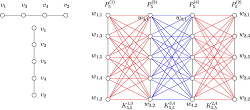
. is the graph
as an example. Terminologies and notations not defined here can be found in [Citation15] for graph theory in general.
Although the antimagicness of graphs concerning Cartesian product has been explored extensively, there are few results regarding lexicographic product. As far as we know, the only result concerning lexicographic product of graphs is obtained by Wang and Hsiao in [Citation7], which states that
Lemma 2
[Citation7]
If is an antimagic
-regular graph with
, then the lexicographic product graph
is antimagic.
Notice that the antimagicness of regular graphs has been obtained in [Citation3] and [Citation4] respectively. So, the result in Lemma 2 can be extended as
Lemma 3
If is a
-regular graph with
, then the lexicographic product graph
is antimagic.
But, except for Lemma 3, there are no other results concerning the antimagicness of lexicographic product of graphs. In this paper, we obtained the following result concerning the antimagicness of the lexicographic product of graphs.
Theorem 1
The lexicographic product graphs are antimagic.
2 The labeling technique for  ()
()
For convenience, throughout this paper, a -path
is represented by a specified sequence
of its vertices, i.e.,
. In graph
, the vertices are represented by
,
,
,
(
). For each
, the vertex set
is called the
-
of
. In
, the vertices
and
are called the endpoints of
, and the other vertices are called the internal vertices of
. The graph
can be decomposed into
copies of the path
and
copies of the complete bipartite graphs
. The
copies of the path
are denoted by
,
,
and
, where
for
. The
copies of the complete bipartite graph
are represented by
(
) and
respectively, where the symbol
stands for the complete bipartite graph between
and
in
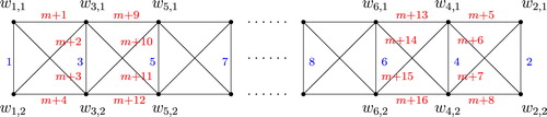
. The symbols mentioned above can be deduced from an example in .
Let be a graph labeling on
, where
is a labeling on the subgraph
of
, and
is a labeling on the subgraph
of
. The following is the technique for graph labeling
on
.
Step 1. The graph labeling on the paths
,
,
and
in
.
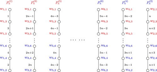
For , the vertex set of
is
, and the edge set of
is
, which is illustrated by . The graph labeling
on the edges of
is defined as follows.
(1)
(1) Therefore, for
, we have
Furthermore, the following monotonic sequences can be deduced from a simple calculation
Step 2. The graph labeling on the complete bipartite graphs
,
,
,
,
,
,
in
.
When Step 1 is completed, we have labeled all the edges in ,
,
and
, and used all the numbers in the set
. In the following, the edge labeling for
(
) is represented in Step 2-1, and the edge labeling for
is represented in Step 2-2.
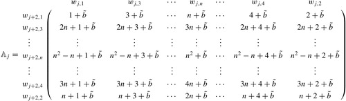
(2-1) For , the graph labeling
on
is represented by the matrix
, and the entry
, which lies in the
th row and
th column of
, represents the number labeled on the edge
through
. The matrix
is defined as
(2)
(2) where
is an
matrix with all entries being 1, and
is the following matrix
For more intuitive,
may be represented as the following, where
.
(2-2) When Step 1 and Step 2-1 are completed, all the numbers in the set {1, 2, ,
} have been used. The graph labeling
on
is represented by the following matrix
.
(3)
(3) where
is a
generalized magic matrix according to Lemma 1. The entry
, which lies in the
th row and
th column of
, indicates the number labeled on the edge
through
.
For , let
denote the sum of the elements in row
of
,
denote the sum of the elements in column
of
. Then
can be represented as
Through the above discussion we can get that, for each vertex of
, the vertex-sum
has the following expression
The following monotonic sequence can be deduced from a simple calculation.
Claim 1
For , the vertex-sum of
,
,
, and
in
satisfies
(4)
(4)
Furthermore, we have the following claims.
Claim 2
The vertex-sums of all the endpoints in satisfy
(5)
(5)
Proof
According to Claim 1, it can be obtained that for
. For
, through the following calculations we can get the inequalities
for
. And thereforeClaim 2 is obtained.
Claim 3
The vertex-sums of all the internal vertices in satisfy
(6)
(6)
Proof
From Claim 1 we can get that for
. In the following, we will prove the inequality
.
From the above, we can get that Claim 3 is obtained.
Claim 4
Under the labeling , if there are two vertices in
whose vertex-sums are equal, then these two vertices must satisfy the property that one is an internal vertex of
and the other is an endpoint of
with
.
Proof
(i) Firstly, we prove that .
From Claims 2 and 3 we can get that the vertex-sums of all endpoints in are pairwise distinct, and that the vertex-sums of all internal vertices in
are also pairwise distinct. So, the two vertices with the same vertex-sum must be that one is an internal vertex of
and the other is an endpoint of
. Furthermore, combiningClaims 1 and 2 we can get that
.
(ii) Secondly, we prove that .
Without loss of generality, we may let , where
is one of the internal vertex of
,
is one of the endpoint of
,
. Through a calculation we can get that
. So, from Claim 2 we can get that the following inequality holds for any
.
Combining this inequality with Claim 3 it can be deduced that if
, then
.
From Claim 4, the following proposition can be easily obtained.
Proposition
For , if there is no internal vertex in
whose vertex-sum is equal to that of an endpoint in
, then the vertex-sums of all vertices in
and
are pair distinct.
The difference between two vertex-sums is called the of the corresponding two vertices. Through some calculations, we can get the following claim.
Claim 5
(i) The footstep between two endpoints is (7)
(7)
(8)
(8)
(ii) For , the footstep between two internal vertices is
(9)
(9)
(iii) For , the footstep between two internal vertices is
(10)
(10)
Claim 6
Let ,
.
(i) If ,
and
, then
,
and
, i.e., if
and
are the two endpoints of
, then
and
must be the last two internal vertices of
. Furthermore,
.
(ii) If ,
, furthermore
is one of the endpoints of
,
is one of the endpoints of
, then
and
must be internal vertices of
and they are separated by at least two other internal vertices of
.
Proof
Because and
, so we have
(11)
(11)
(i) In this case, without loss of generality, we may let and
. Since
and
, it can be obtained from Claim 4 that
and
must be internal vertices of
and
respectively, furthermore both
and
are less than
. If
, then according to Claim 3 and the relations (Equation7
(7)
(7) ), (Equation9
(9)
(9) ) and (Equation10
(10)
(10) ) we can get that
which contradicts the relation (Equation11
(11)
(11) ). Therefore it can be deduced that
, i.e., both
and
are internal vertices of
. Furthermore, combining (Equation11
(11)
(11) ) we can get that
. Now, if
, then it can be deduced from Claim 3 and the relations (Equation7
(7)
(7) ), (Equation9
(9)
(9) ) and (Equation10
(10)
(10) ) that
which contradicts to the relation (Equation11
(11)
(11) ). So it can be obtained that
, and therefore
. On the other hand,
. So, combining (Equation11
(11)
(11) ) it can be deduced that
and
must be the last two internal vertices
and
in
. And Claim 6 (i) is obtained.
(ii) In this case, let . Since
, the vertex
is denoted by
. According to Claim 4 it can be deduced that both
and
are internal vertices of
, furthermore
. Because
and
are endpoints of
and
respectively, according to (Equation8
(8)
(8) ) and (Equation11
(11)
(11) ) and Claim 2 we can get that
(12)
(12) On the other hand, since
, combining with (Equation8
(8)
(8) )–(Equation10
(10)
(10) ) it can be obtained that for
From (Equation12
(12)
(12) ) we can get that
, and so
which indicates that
and
are separated by at least two other vertices of
, and Claim 6 (ii) is obtained.
Under the labeling , if there are two vertices whose vertex-sums are equal, then the following two ways of modification can change them into unequal.
Modification on the labeling : Let
be an internal vertex of
and
be an endpoint of
with
. If
, then the following two ways of modification can make
hold.
Modification-: In this case, the labeling
is illustrated by the left of , where
denotes the internal vertex which belongs to
. The Modification-
is choosing any vertex
from
, and then exchanging the labels on edges
and
. According to the expression (Equation2
(2)
(2) ) it can be obtained that, after the Modification
,
increases by
,
decreases by
, but the vertex-sums of all the other vertices remain unchanged.
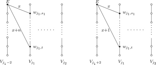
Modification-: In this case, the labeling
is illustrated by the right of , where
denotes the internal vertex which belongs to
. The Modification-
is choosing any vertex
from
, and then exchanging the labels on edges
and
. According to the expression (Equation2
(2)
(2) ) it can be obtained that, after the Modification
,
increases by
,
decreases by
, but the vertex-sums of all the other vertices remain unchanged.
3 Proof of Theorem 1
Proof
The proof of Theorem 1 is discussed in the following three cases according to ,
, and
respectively.
Case 1. .
Subcase 1.1
In this case, the graph is , and its antimagicness can be easily obtained.
Subcase 1.2
In this case, the graph is decomposed into
,
, and
. Firstly, we use
to label the complete bipartite graph
, and the labeling
is represented by the generalized magic matrix. So we have
Now, we use
to label the edges of
and
. For
, the graph labeling
on the edges of
is defined as
Through a calculation, the following monotonic sequences can be obtained
Since
, from the above it can be obtained that
(13)
(13) Noticing that, for
, we have
(14)
(14) From (Equation13
(10)
(10) ) and (Equation14
(14)
(14) ) we can get the following relation
and the antimagicness of
is obtained.
Case 2.
Subcase 2.1
In this case, the graph is , and its antimagicness can be easily obtained.
Subcase 2.2
In this case, the graph is decomposed into
,
,
,
, and
. The labeling
is given by the expression (Equation1
(1)
(1) ),
is given by the expressions (Equation2
(2)
(2) ) and (Equation3
(3)
(3) ), where
According to Claim 1 it can be obtained that
(15)
(15) For
, the following relations (Equation16
(15)
(15) ) and (Equation17
) can be obtained through some calculations
(16)
(16)
(17)
(17) From (Equation15
(15)
(15) )–(Equation17
(17)
(17) ) we can get the following relation
and the antimagicness of
is obtained.
Case 3.
Subcase 3.1
In this case, the graph is . The antimagicness of
can be easily obtained from the labeling illustrated by .
Subcase 3.2
In this case, the graph is decomposed into
,
, …,
,
,
,
, and
,
,
,
,
,
,
. The labeling
is given by the expression (Equation1
(1)
(1) ),
is given by the expressions (Equation2
(2)
(2) ) and (Equation3
(3)
(3) ), where
According to Claim 2 it can be obtained that the vertex-sums of all endpoints in this case satisfy the relation (Equation5
(5)
(5) ). Furthermore, through some calculations we can get that the vertex-sums of all internal vertices in this case satisfy
(18)
(18) So, if there is no endpoint whose vertex-sum equals one of the internal vertex’s vertex-sum, then the antimagicness of
is obtained. If there exists an endpoint whose vertex-sum is equal to that of an internal vertex, say,
with
according to Claim 4, then the antimagicness of
can be obtained from one of the following two methods.
Method- 1: Exchanging the labeling on the edges and
.
After the exchanging, the vertex-sums of and
have been changed and denoted by
and
respectively, but the vertex-sums of all the other vertices remain unchanged. It can be obtained that
Furthermore, from the relations (Equation5
(5)
(5) ) and (Equation18
) and some calculations we can get that
Method- 2: Exchanging the labeling on the edges and
Similar to that of the method-1, we can get that and
in this case satisfy the following relations.
Furthermore, from the relations (Equation5
(5)
(5) ) and (Equation18
) and some calculations we can get that
Keep Claims 4 and 6 (i) in mind, and repeat the above process if there are still other pairs of vertex-sum being equal. From the above discussion we can get the antimagicness of .
Subcase 3.3
In this case, the graph is decomposed into
copies of the path
,
,
,
,
,
,
, and
copies of the complete bipartite graphs
,
,
,
,
,
,
. The labeling
is given by the expression (Equation1
(1)
(1) ),
is given by the expressions (Equation2
(2)
(2) ) and (Equation3
(3)
(3) ), where
For convenience, the endpoint’s vertex-sums
,
,
,
,
,
, and
are represented by
,
,
,
,
and
respectively. The internal vertex’s vertex-sums
,
,
,
,
,
,
,
,
,
,
,
,
are represented by
,
,
,
,
respectively. Let
,
. According to Claims 2 and 3, it can be obtained that the elements in
and
satisfy the following two monotonic sequences.
Step 1.
In , if there exist two elements
and
being the vertex-sums of the two endpoints in the same
, where
according to Claim 4, then from Claim 6 (i) we can get that
and
must be the last two internal vertices of
with
, i.e.,
Now, make the Modification
on
, i.e., choose any vertex
from
and then exchange the labels on edges
and
. After the Modification
,
and
are replaced by
and
respectively, where
,
, but the vertex-sums of all the other vertices remain unchanged. According to the relation (Equation10
(10)
(10) ) it can be obtained that the footstep between
and
is
Therefore
, and the following relation can be obtained
(19)
(19) Noticing that
and
are the vertex-sums of the two endpoints in
,
and
are the vertex-sums of the last two internal vertices in
, combining (Equation5
(5)
(5) ), (Equation6
(6)
(6) ) and (Equation19
(19)
(19) ) it can be deduced that there is no element in
and
being equal to
or
.
If there are still other pair of elements in , say,
and
, being the vertex-sums of the two endpoints in the same
(
according to Claim 4), then repeat the above modification process, and so on.
Step 2.
After the Step 1, if the elements in and
are pairwise distinct, then the antimagicness of
can be obtained. If there still exist some elements in
which are equal to some elements in
respectively, then these elements in
and
are denoted by
and
respectively, where
for
. Without loss of generality, let the elements in
and
satisfy the following two monotonic sequences.
Let and
be the elements selected arbitrarily from
and
respectively. Without loss of generality, we may let
,
, i.e.,
where
,
,
.
(i) If and
, i.e.,
is one of the endpoints in
and
is one of the internal vertices in
, then make the Modification
on
, that is to say, choose any vertex
from
and then exchange the labels on edges
and
, where
is one of
which belongs to
.
(ii) If and
, then make the Modification
on
, that is to say, choose any vertex
from
and then exchange the labels on edges
and
, where
is one of
which belongs to
.
(iii) If , then make the Modification
on
, that is to say, choose any vertex
from
and then exchange the labels on edges
and
, where
is one of
which belongs to
.
Make the above modification on all elements in . After the Modification
(or
),
, increases by
(or 1), and
, decreases by
(or 1), but the vertex-sums of all the other vertices remain unchanged. Let
and
denote, after the Modification A (or B), the vertex-sums of
and
respectively. In the following we will show that, after the modification, no elements in
and
can be equal to
or
, and therefore the antimagicness of
can be deduced.
The proof methods for (i), (ii) and (iii) are similar, and here we only give the proof for (iii). Without loss of generality, we may let and the modification be of type
. After the Modification
, the vertex-sum
of
increases by
and changed into
, the vertex-sum
of
decreases by
and changed into
. For convenience of expression, the elements in
and
are represented by the following.
(20)
(20) Since
, according to the relations (Equation7
(7)
(7) ,Equation8
(8)
(8) ) we can get that the footstep between the two endpoints
and
is
(21)
(21) And according to the relations (Equation9
(9)
(9) ) and (Equation10
(10)
(10) ) we can get that
(22)
(22) From the relation (Equation22
(22)
(22) ) it can be obtained that
So, the following inequality can be obtained
(23)
(23) Since
, combining with (Equation21
(21)
(21) ) and (Equation22
(22)
(22) ) it can be obtained that
So,
. Combining this inequality with (Equation20
(20)
(20) ) and (Equation23
(23)
(23) ) it can be obtained that
(24)
(24) By comparing (Equation20
(20)
(20) ) with (Equation24
(24)
(24) ) it can be obtained that there is no element in
and
being equal to
or
.
Notes
This work was supported by the National Natural Science Foundation of China (Grant Nos. 11401430 and 11301381).
Peer review under responsibility of Kalasalingam University.
References
- Hartsfield N. Ringel G. Pearls in Graph Theory: A Comprehensive Introduction 1990 Academic Press Boston 108 110
- Alon N. Kaplan G. Lev A. Roditty Y. Yuster R. Dense graphs are antimagic J. Graph Theory 47 4 2004 297 309
- Chang F. Liang Y. Pan Z. Zhu X. Antimagic labeling of regular graphs J. Graph Theory 82 4 2016 339 349
- Bérczi K. Bernáth A. Vizer M. Regular graphs are antimagic Electron. J. Combin. 22 3 2015 ♯ P3.34
- Kaplan G. Lev A. Roditty Y. On zero-sum partitions and anti-magic trees Discrete Math. 309 2009 2010 2014
- Liang Y. Wong T. Zhu X. Anti-magic labeling of trees Discrete Math. 331 2014 9 14
- Wang T. Hsiao C. On anti-magic labeling for graph products Discrete Math. 308 2008 3624 3633
- Wang T. Liu M. Li D. A class of antimagic join graphs Acta Math. Sin. English Ser. 29 5 2013 1019 1026
- Bača M. Phanalasy O. Ryan J. Antimagic labelings of join graphs Math. Comput. Sci. 9 2 2015 139 143
- Arumugam S. Miller M. Phanalasy O. Antimagic labeling of generalized pyramid graphs Acta Math. Sin. (Engl. Ser.) 30 2 2014 283 290
- Hefetz D. Mutze T. Schwartz J. On antimagic directed graphs J. Graph Theory 64 3 2010 219 232
- Arumugam S. Premalatha K. Bača M. Local antimagic vertex coloring of a graph Graphs Combin. 33 2 2017 1 11
- Gallian J.A. A dynamic survey of graph labeling Electron. J Combin. 2014 384pp., ♯ DS6 (17th ed)
- Pasles P.C. Benjamin Franklin’S Numbers 2008 Princeton University Press Princeton, NJ
- West D. Introduction of Graph Theory second ed. 2001 Prentice Hall