Normalized Laplacian spectrum of some subdivision-joins and R-joins of two regular graphs

Peer review under responsibility of Kalasalingam University.

Abstract

In this paper we determine the full normalized Laplacian spectrum of the subdivision-vertex join, subdivision-edge join, $R$-vertex join, and $R$-edge join of two regular graphs in terms of the normalized Laplacian eigenvalues of the graphs. Moreover, applying these results we find non-regular normalized Laplacian cospectral graphs.

Keywords:

• Normalized Laplacian matrix
• Subdivision-vertex join
• Subdivision-edge join
• $R$-vertex join
• $R$-edge join

1 Introduction

The theory of graph spectra has numerous applications in several areas of science and technology. There are several kinds of spectra associated with a graph and they characterize many properties of the graph. Here we are interested on normalized Laplacian spectrum of a graph. This spectrum checks several structural properties of a graph including bipartiteness and connectedness. Chung [1] introduced the normalized Laplacian matrix $\mathcal{L}\left(G\right)$ of a simple graph $G$. This matrix $\mathcal{L}\left(G\right)$ is a square matrix with rows and columns indexed by vertices of $G$, and for any two vertices $u$ and $v$ the ${(u,v)}^{th}$ entry of $\mathcal{L}\left(G\right)$ is given by $\mathcal{L}(u,v)=\left\{\begin{array}{cc}\hfill & 1\text{if}u=v\text{and}{d}_v\ne 0\text{,}\hfill \\ \hfill & \frac{-1}{\sqrt{d_u{d}_v}}\text{if}u\text{and}v\text{are adjacent},\hfill \\ \hfill & 0\text{otherwise},\hfill \end{array}\right.$where $d_u$ and $d_v$ are degrees of $u$ and $v$ respectively. If $D\left(G\right)$ is the diagonal matrix of vertex degrees and $A\left(G\right)$ is the adjacency matrix of $G$, where $A(u,v)=1$ if and only if vertex $u$ is adjacent to vertex $v$ and $0$ otherwise, then we can write $\mathcal{L}\left(G\right)=I-D{\left(G\right)}^{-1∕2}A\left(G\right)D{\left(G\right)}^{-1∕2}$ with the convention that $D{\left(G\right)}^{-1}(u,u)=0$ if $d_u=0$. We denote the characteristic polynomial $\det (\lambda I-\mathcal{L}\left(G\right))$ of $\mathcal{L}\left(G\right)$ by $f_G\left(\lambda \right)$. The roots of $f_G\left(\lambda \right)$ are known as the normalized Laplacian eigenvalues of $G$. The multiset of the normalized Laplacian eigenvalues of $G$ is called the normalized Laplacian spectrum of $G$. Since $\mathcal{L}\left(G\right)$ is a symmetric and positive semi-definite matrix, its eigenvalues, denoted by ${\lambda }_1\left(G\right),{\lambda }_2\left(G\right),\dots ,{\lambda }_n\left(G\right)$, are all real, non-negative and can be arranged in non-decreasing order ${\lambda }_1\left(G\right)\le {\lambda }_2\left(G\right)\le \cdots \le {\lambda }_n\left(G\right)$. In [1], Chung proved that all normalized Laplacian eigenvalues of a graph lie in the interval $[0,2]$, and $0$ is always a normalized Laplacian eigenvalue, that is ${\lambda }_1\left(G\right)=0$. She also determined normalized Laplacian spectrum of different kinds of graphs like complete graphs, bipartite graphs, hypercubes etc. Two graphs $G$ and $H$ are called cospectral if $A\left(G\right)$ and $A\left(H\right)$ have the same spectrum. Similarly, graphs $G$ and $H$ are called normalized Laplacian cospectral or simply $\mathcal{L}$-cospectral if the spectrum of $\mathcal{L}\left(G\right)$ and $\mathcal{L}\left(H\right)$ are the same. Banerjee and Jost [2] investigated how the normalized Laplacian spectrum is affected by operations like motif doubling, graph splitting or joining. In [3], Butler and Grout produced (exponentially) large families of non-bipartite, non-regular graphs which are mutually cospectral, and also gave an example of a graph which is cospectral with its complement but is not self-complementary. In [4], Li studied the effect on the second smallest normalized Laplacian eigenvalue by grafting some pendant paths. The join [5] of two graphs is their disjoint union together with all the edges that connect all the vertices of the first graph with all the vertices of the second graph. In [6], Butler computed the normalized Laplacian spectrum for joining of two regular graphs. The subdivision graph $S\left(G\right)$ [7] of a graph $G$ is the graph obtained from $G$ by inserting a new vertex into every edge of $G$. Xie et al. [8] determined the normalized Laplacian spectrum of iterated subdivisions of simple connected graphs. The $R$-graph $\mathcal{R}\left(G\right)$ [9] of a graph $G$ is the graph obtained from $G$ by introducing a new vertex $u_e$ for each $e\in E\left(G\right)$ and making $u_e$ adjacent to both the end vertices of $e$. The set of such new vertices is denoted by $I\left(G\right)$ i.e $I\left(G\right)=V\left(S\left(G\right)\right)\setminus V\left(G\right)=V\left(\mathcal{R}\left(G\right)\right)\setminus V\left(G\right)$. In this paper we are interested on finding normalized Laplacian spectrum of some subdivision-joins and $R$-joins of graphs, which are defined below.

Definition 1.1

Let $G_1$ and $G_2$ be two vertex-disjoint graphs with number of vertices $n_1$ and $n_2$, and edges $m_1$ and $m_2$, respectively. Then

(i) The subdivision-vertex join [10] of $G_1$ and $G_2$, denoted by $G_1\dot{\vee }{G}_2$, is the graph obtained from $S\left(G_1\right)$ and $G_2$ by joining each vertex of $V\left(G_1\right)$ with every vertex of $V\left(G_2\right)$. The graph $G_1\dot{\vee }{G}_2$ has $n_1+n_2+m_1$ vertices and $2m_1+n_1{n}_2+m_2$ edges.

(ii) The subdivision-edge join [10] of $G_1$ and $G_2$, denoted by $G_1⊻G_2$, is the graph obtained from $S\left(G_1\right)$ and $G_2$ by joining each vertex of $I\left(G_1\right)$ with every vertex of $V\left(G_2\right)$. The graph $G_1⊻G_2$ has $n_1+n_2+m_1$ vertices and $m_1(2+n_2)+m_2$ edges.

(iii) The $R$-vertex join [11] of $G_1$ and $G_2$, denoted by $G_1〈\mathrm{v}〉G_2$, is the graph obtained from $\mathcal{R}\left(G_1\right)$ and $G_2$ by joining each vertex of $V\left(G_1\right)$ with every vertex of $V\left(G_2\right)$. The graph $G_1〈\mathrm{v}〉G_2$ has $n_1+n_2+m_1$ vertices and $3m_1+n_1{n}_2+m_2$ edges.

(iv) The $R$-edge join [11] of $G_1$ and $G_2$, denoted by $G_1〈\mathrm{e}〉G_2$, is the graph obtained from $\mathcal{R}\left(G_1\right)$ and $G_2$ by joining each vertex of $I\left(G_1\right)$ with every vertex of $V\left(G_2\right)$. The graph $G_1〈\mathrm{e}〉G_2$ has $n_1+n_2+m_1$ vertices and $m_1(3+n_2)+m_2$ edges.

In [12], Indulal computed adjacency spectra of $G_1\dot{\vee }{G}_2$ and $G_1⊻G_2$ for two regular graphs $G_1$ and $G_2$ in terms of their spectra. In [10], Liu and Zhang determined the adjacency spectrum, Laplacian spectrum and signless Laplacian spectrum of $G_1\dot{\vee }{G}_2$ and $G_1⊻G_2$ for a regular graph $G_1$ and an arbitrary graph $G_2$ in terms of the corresponding spectra of $G_1$ and $G_2$ and also constructed infinite pairs of cospectral graphs. Liu et al. [11] formulated the resistance distances and Kirchoff index of $G_1〈\mathrm{v}〉G_2$ and $G_1〈\mathrm{e}〉G_2$ respectively. For two regular graphs $G_1$ and $G_2$, here we determine the normalized Laplacian spectrum of $G_1\dot{\vee }{G}_2$, $G_1⊻G_2$, $G_1〈\mathrm{v}〉G_2$ and $G_1〈\mathrm{e}〉G_2$ in terms of the normalized Laplacian eigenvalues of $G_1$ and $G_2$. Moreover, we construct non-regular $\mathcal{L}$-cospectral graphs by applying the spectra of the above subdivision-joins and $R$-joins of graphs.

To prove our main results we need the following matrix product and some basic properties on matrices. We recall that for two matrices $A$ and $B$, of same size $m\times n$, the Hadamard product $A•B$ of $A$ and $B$ is a matrix of the same size $m\times n$ with entries given by ${(A•B)}_{ij}={\left(A\right)}_{ij}\cdot {\left(B\right)}_{ij}$ (that is entrywise multiplication).

Lemma 1.1

Schur Complement [7]

Suppose that the order of all four matrices $M$, $N$, $P$ and $Q$ satisfies the rules of operations on matrices. Then we have,

Notation 1.1

Throughout the paper for any integer $n$, $I_n$ denotes the $n\times n$ identity matrix, $J_{n\times n}$ denotes $n\times n$ matrix whose all entries equal to $1$, and ${\mathbf{1}}_n$ stands for the column vector of size $n$ with all entries equal to $1$, $K_{n\times n}$ denotes an $n\times n$ matrix whose all entries are equal, and $C_n$ denotes a column vector of $K_{n\times n}$. In other words, $K_{n\times n}=\alpha J_{n\times n}$ and $C_n=\alpha {\mathbf{1}}_n$, for a real number $\alpha$. For any positive integers $s$ and $t$, $O_{s\times t}$ denotes the zero matrix of size $s\times t$.

The Lemma below can be obtained easily.

Lemma 1.2

For a square matrix $A$ of size $n$ and a scalar $\alpha$, $\det (A+\alpha J_{n\times n})=\det \left(A\right)+\alpha {\mathbf{1}}_n^{T}adj\left(A\right){\mathbf{1}}_n,$where $adj\left(A\right)$ is the adjugate matrix of $A$.

For a graph $G$ with $n$ vertices and $m$ edges, the vertex-edge incidence matrix $R\left(G\right)$ [13] is a matrix of order $n\times m$, with entry $r_{ij}=1$ if the $i$th vertex is incident to the $j$th edge, and $0$ otherwise. The line graph [13] of a graph $G$ is the graph $L\left(G\right)$, whose vertices are the edges of $G$ and two vertices of $L\left(G\right)$ are adjacent if and only if they have a common end vertex in $G$. It is well known [7] that $R{\left(G\right)}^{T}R\left(G\right)=A\left(L\left(G\right)\right)+2I_m$. In particular, if $G$ is an $r$-regular graph then $R\left(G\right)R{\left(G\right)}^T=A\left(G\right)+r{I}_n$.

Lemma 1.3

[7]

Let $G$ be an $r-$regular graph. Then the eigenvalues of $A\left(L\left(G\right)\right)$ are the eigenvalues of $A\left(G\right)+(r-2)I_n$, and $-2$ repeated $m-n$ times.

If $G$ is an $r-$regular graph, then obviously $\mathcal{L}\left(G\right)=I_n-\frac{1}{r}A\left(G\right)$. Therefore, by Lemma 1.3, we have the following.

Lemma 1.4

For an $r-$regular graph $G$, the eigenvalues of $A\left(L\left(G\right)\right)$ are the eigenvalues of $2(r-1)I_n-r\mathcal{L}\left(G\right)$, and $-2$ repeated $m-n$ times.

2 Our results

In the lemma below we represent the normalized Laplacian matrix of subdivision-vertex join, subdivision-edge join, $R$-vertex join and $R$-edge join of two regular graphs in terms of Hadamard product of matrices. For $i=1,2$, let $G_i$ be a graph with $n_i$ vertices and $m_i$ edges. Let $V\left(G_1\right)=\{v_1,\dots ,v_{n_1}\}$, $I\left(G_1\right)=\{e_1,\dots ,e_{m_1}\}$ and $V\left(G_2\right)=\{u_1,\dots ,u_{n_2}\}$. Then $V\left(G_1\right)\cup I\left(G_1\right)\cup V\left(G_2\right)$ is a partition of $V\left(G_1\dot{\vee }{G}_2\right)$, $V(G_1⊻G_2)$, $V\left(G_1〈\mathrm{v}〉G_2\right)$ and $V\left(G_1〈\mathrm{e}〉G_2\right)$. The degrees of the vertices in $G_1\dot{\vee }{G}_2$ are $d_{G_1\dot{\vee }{G}_2}\left(v_i\right)=d_{G_1}\left(v_i\right)+n_2$, $d_{G_1\dot{\vee }{G}_2}\left(e_i\right)=2$ and $d_{G_1\dot{\vee }{G}_2}\left(u_i\right)=d_{G_2}\left(u_i\right)+n_1$. The degrees of the vertices in $G_1⊻G_2$ are $d_{G_1⊻G_2}\left(v_i\right)=d_{G_1}\left(v_i\right)$, $d_{G_1⊻G_2}\left(e_i\right)=2+n_2$ and $d_{G_1⊻G_2}\left(u_i\right)=d_{G_2}\left(u_i\right)+m_1$. The degrees of the vertices in $G_1〈\mathrm{v}〉G_2$ are $d_{G_1〈\mathrm{v}〉G_2}\left(v_i\right)=2d_{G_1}\left(v_i\right)+n_2$, $d_{G_1〈\mathrm{v}〉G_2}\left(e_i\right)=2$ and $d_{G_1〈\mathrm{v}〉G_2}\left(u_i\right)=d_{G_2}\left(u_i\right)+n_1$. The degrees of the vertices in $G_1〈\mathrm{e}〉G_2$ are $d_{G_1〈\mathrm{e}〉G_2}\left(v_i\right)=2d_{G_1}\left(v_i\right)$, $d_{G_1〈\mathrm{e}〉G_2}\left(e_i\right)=2+n_2$ and $d_{G_1〈\mathrm{e}〉G_2}\left(u_i\right)=d_{G_2}\left(u_i\right)+m_1$.

Lemma 2.1

For $i=1,2$, let $G_i$ be an $r_i$-regular graph with $n_i$ vertices and $m_i$ edges. Then we have the following:

(i) $\mathcal{L}\left(G_1\dot{\vee }{G}_2\right)=\left(\begin{array}{ccc}\hfill I_{n_1}\hfill & \hfill -cR\left(G_1\right)\hfill & \hfill -K_{n_1\times n_2}\hfill \\ \hfill -cR{\left(G_1\right)}^T\hfill & \hfill I_{m_1}\hfill & \hfill O_{m_1\times n_2}\hfill \\ \hfill -K_{n_2\times n_1}\hfill & \hfill O_{n_2\times m_1}\hfill & \hfill \mathcal{L}\left(G_2\right)•B\left(G_2\right)\hfill \end{array}\right)$where $K_{n_1\times n_2}$ is the matrix of size $n_1\times n_2$ with all entries equal to $\frac{1}{\sqrt{(r_1+n_2)(r_2+n_1)}}$, $B\left(G_2\right)$ is the $n_2\times n_2$ matrix whose all diagonal entries are $1$ and off-diagonal entries are $\frac{r_2}{r_2+n_1}$, $c$ is the constant whose value is $\frac{1}{\sqrt{2(r_1+n_2)}}$.

(ii) $\mathcal{L}(G_1⊻G_2)=\left(\begin{array}{ccc}\hfill I_{n_1}\hfill & \hfill -cR\left(G_1\right)\hfill & \hfill O_{n_1\times n_2}\hfill \\ \hfill -cR{\left(G_1\right)}^T\hfill & \hfill I_{m_1}\hfill & \hfill -K_{m_1\times n_2}\hfill \\ \hfill O_{n_2\times n_1}\hfill & \hfill -K_{n_2\times m_1}\hfill & \hfill \mathcal{L}\left(G_2\right)•B\left(G_2\right)\hfill \end{array}\right)$where $K_{m_1\times n_2}$ is the matrix of size $m_1\times n_2$ with all entries equal to $\frac{1}{\sqrt{(2+n_2)(r_2+m_1)}}$, $B\left(G_2\right)$ is the $n_2\times n_2$ matrix whose all diagonal entries are $1$ and off-diagonal entries are $\frac{r_2}{r_2+m_1}$, $c$ is the constant whose value is $\frac{1}{\sqrt{r_1(2+n_2)}}$.

(iii) $\mathcal{L}\left(G_1〈\mathrm{v}〉G_2\right)=\left(\begin{array}{ccc}\hfill \mathcal{L}\left(G_1\right)•B\left(G_1\right)\hfill & \hfill -cR\left(G_1\right)\hfill & \hfill -K_{n_1\times n_2}\hfill \\ \hfill -cR{\left(G_1\right)}^T\hfill & \hfill I_{m_1}\hfill & \hfill O_{m_1\times n_2}\hfill \\ \hfill -K_{n_2\times n_1}\hfill & \hfill O_{n_2\times m_1}\hfill & \hfill \mathcal{L}\left(G_2\right)•B\left(G_2\right)\hfill \end{array}\right)$where $K_{n_1\times n_2}$ is the matrix of size $n_1\times n_2$ with all entries equal to $\frac{1}{\sqrt{(2r_1+n_2)(r_2+n_1)}}$, $B\left(G_1\right)$ is the $n_1\times n_1$ matrix whose all diagonal entries are $1$ and off-diagonal entries are $\frac{r_1}{2r_1+n_2}$, $B\left(G_2\right)$ is the $n_2\times n_2$ matrix whose all diagonal entries are $1$ and off-diagonal entries are $\frac{r_2}{r_2+n_1}$, $c$ is the constant whose value is $\frac{1}{\sqrt{2(2r_1+n_2)}}$.

(iv) $\mathcal{L}\left(G_1〈\mathrm{e}〉G_2\right)=\left(\begin{array}{ccc}\hfill \mathcal{L}\left(G_1\right)•B\left(G_1\right)\hfill & \hfill -cR\left(G_1\right)\hfill & \hfill O_{n_1\times n_2}\hfill \\ \hfill -cR{\left(G_1\right)}^T\hfill & \hfill I_{m_1}\hfill & \hfill -K_{m_1\times n_2}\hfill \\ \hfill O_{n_2\times n_1}\hfill & \hfill -K_{n_2\times m_1}\hfill & \hfill \mathcal{L}\left(G_2\right)•B\left(G_2\right)\hfill \end{array}\right)$where $K_{m_1\times n_2}$ is the matrix of size $m_1\times n_2$ with all entries equal to $\frac{1}{\sqrt{(2+n_2)(r_2+m_1)}}$, $B\left(G_1\right)$ is the $n_1\times n_1$ matrix whose all diagonal entries are $1$ and off-diagonal entries are $\frac{r_1}{2r_1}$, $B\left(G_2\right)$ is the $n_2\times n_2$ matrix whose all diagonal entries are $1$ and off-diagonal entries are $\frac{r_2}{r_2+m_1}$, $c$ is the constant whose value is $\frac{1}{\sqrt{2r_1(2+n_2)}}$.

Definition 2.1

[14,15]

The $M$-coronal ${\Gamma }_M\left(x\right)$ of an $n\times n$ matrix $M$ is defined as the sum of the entries of the matrix ${(x{I}_n-M)}^{-1}$(if exists), that is, ${\Gamma }_M\left(x\right)={\mathbf{1}}_n^T{(x{I}_n-M)}^{-1}{\mathbf{1}}_n.$

The following Lemma is straightforward.

Lemma 2.2

[14]

If $M$ is an $n\times n$ matrix with each row sum equal to a constant $t$, then ${\Gamma }_M\left(x\right)=\frac{n}{x-t}$.

Notation 2.1

For an $n$ vertex graph $G$ be a graph on $n$ vertices, matrices $B$ and $C$ of sizes $n\times n$ and $n\times 1$ respectively, and a parameter $\lambda$, we have the notation: ${\chi }_G(B,C,\lambda )=C^T{(\lambda I_n-(\mathcal{L}\left(G\right)•B))}^{-1}C$. We note that the notation is similar to the notion ‘coronal’.

In the next four theorems we find spectra of all join graphs considered in the paper. In all these theorems we take that for $i=1,2$, $G_i$ is an $r_i$-regular graph with $n_i$ vertices and $m_i$ edges.

Theorem 2.1

The normalized Laplacian spectrum of $G_1\dot{\vee }{G}_2$ consists of:

(i)	The eigenvalue $\frac{n_1+r_2{\delta }_j}{r_2+n_1}$, for every eigenvalue ${\delta }_j$ $(j=2,3,\dots ,n_2)$ of $\mathcal{L}\left(G_2\right)$,

(ii)	The eigenvalue $1$ with multiplicity $m_1-n_1$,

(iii)

Two roots of the equation $2(r_1+n_2){\lambda }^2-4(r_1+n_2)\lambda +2n_2+r_1{\mu }_i=0$, for each eigenvalue ${\mu }_i$ $(i=2,3,\dots ,n_1)$ of $\mathcal{L}\left(G_1\right)$,

(iv)	Three roots of the equation $(r_1{r}_2+r_1{n}_1+r_2{n}_2+n_1{n}_2){\lambda }^3-(2r_1{r}_2+3r_1{n}_1+2r_2{n}_2+3n_1{n}_2){\lambda }^2+(2r_1{n}_1+r_2{n}_2+2n_1{n}_2)\lambda =0$.

Proof

The normalized Laplacian characteristic polynomial of $G_1\dot{\vee }{G}_2$ is $f_{G_1\dot{\vee }{G}_2}\left(\lambda \right)=\det (\lambda I_{n_1+n_2+m_1}-\mathcal{L}\left(G_1\dot{\vee }{G}_2\right))=\det \left(\begin{array}{ccc}\hfill (\lambda -1)I_{n_1}\hfill & \hfill cR\left(G_1\right)\hfill & \hfill K_{n_1\times n_2}\hfill \\ \hfill cR{\left(G_1\right)}^T\hfill & \hfill (\lambda -1)I_{m_1}\hfill & \hfill O_{m_1\times n_2}\hfill \\ \hfill K_{n_2\times n_1}\hfill & \hfill O_{n_2\times m_1}\hfill & \hfill \lambda I_{n_2}-(\mathcal{L}\left(G_2\right)•B\left(G_2\right))\hfill \end{array}\right)=\det (\lambda I_{n_2}-(\mathcal{L}\left(G_2\right)•B\left(G_2\right)))\det \left(S\right),$where $S=\left(\begin{array}{cc}\hfill (\lambda -1)I_{n_1}\hfill & \hfill cR\left(G_1\right)\hfill \\ \hfill cR{\left(G_1\right)}^T\hfill & \hfill (\lambda -1)I_{m_1}\hfill \end{array}\right)-\left(\begin{array}{c}\hfill K_{n_1\times n_2}\hfill \\ \hfill O_{m_1\times n_2}\hfill \end{array}\right){(\lambda I_{n_2}-(\mathcal{L}\left(G_2\right)•B\left(G_2\right)))}^{-1}\left(\begin{array}{cc}\hfill K_{n_2\times n_1}\hfill & \hfill O_{n_2\times m_1}\hfill \end{array}\right)=\left(\begin{array}{cc}\hfill (\lambda -1)I_{n_1}-{\chi }_{G_2}(B\left(G_2\right),C_{n_2},\lambda )J_{n_1\times n_1}\hfill & \hfill cR\left(G_1\right)\hfill \\ \hfill cR{\left(G_1\right)}^T\hfill & \hfill (\lambda -1)I_{m_1}\hfill \end{array}\right).$ Then $\begin{array}{ccc}\hfill \det \left(S\right)& \hfill =\hfill & {(\lambda -1)}^{m_1}\det ((\lambda -1)I_{n_1}-{\chi }_{G_2}(B\left(G_2\right),C_{n_2},\lambda )J_{n_1\times n_1}-\frac{c^2}{\lambda -1}R\left(G_1\right)R{\left(G_1\right)}^T)\hfill \\ \hfill & \hfill =\hfill & {(\lambda -1)}^{m_1}[\det ((\lambda -1)I_{n_1}-\frac{c^2}{\lambda -1}R\left(G_1\right)R{\left(G_1\right)}^T)\hfill \\ \hfill & \hfill \hfill & -{\chi }_{G_2}(B\left(G_2\right),C_{n_2},\lambda ){\mathbf{1}}_{n_1}^{T}adj\{(\lambda -1)I_{n_1}-\frac{c^2}{\lambda -1}R\left(G_1\right)R{\left(G_1\right)}^T\}{\mathbf{1}}_{n_1}]\hfill \\ \hfill & \hfill =\hfill & {(\lambda -1)}^{m_1}\det ((\lambda -1)I_{n_1}-\frac{c^2}{\lambda -1}R\left(G_1\right)R{\left(G_1\right)}^T)\hfill \\ \hfill & \hfill \hfill & [1-{\chi }_{G_2}(B\left(G_2\right),C_{n_2},\lambda ){\mathbf{1}}_{n_1}^T{\{(\lambda -1)I_{n_1}-\frac{c^2}{\lambda -1}R\left(G_1\right)R{\left(G_1\right)}^T\}}^{-1}{\mathbf{1}}_{n_1}]\hfill \\ \hfill & \hfill =\hfill & {(\lambda -1)}^{m_1}\det ((\lambda -1)I_{n_1}-\frac{c^2}{\lambda -1}{r}_1(2I_{n_1}-\mathcal{L}\left(G_1\right)))[1-{\chi }_{G_2}(B\left(G_2\right),C_{n_2},\lambda ){\Gamma }_{\frac{c^2}{\lambda -1}R\left(G_1\right)R{\left(G_1\right)}^T}(\lambda -1)].\hfill \end{array}$Since $\mathcal{L}\left(G_2\right)•B\left(G_2\right)=I_{n_2}-\frac{1}{r_2+n_1}A\left(G_2\right)$, we get $\mathcal{L}\left(G_2\right)•B\left(G_2\right)=\frac{1}{r_2+n_1}(n_1{I}_{n_2}+r_2\mathcal{L}\left(G_2\right))$.

As $G_2$ is regular, the sum of all entries on every row of its normalized Laplacian matrix is zero. That means $\mathcal{L}\left(G_2\right)C_{n_2}=(1-\frac{r_2}{r_2})C_{n_2}=0C_{n_2}$. Then $(\mathcal{L}\left(G_2\right)•B\left(G_2\right))C_{n_2}=(1-\frac{r_2}{r_2+n_1})C_{n_2}=\frac{n_1}{r_2+n_1}{C}_{n_2}$ and $(\lambda I_{n_2}-(\mathcal{L}\left(G_2\right)•B\left(G_2\right)))C_{n_2}=(\lambda -\frac{n_1}{r_2+n_1})C_{n_2}$. Also, $C_{n_2}^T{C}_{n_2}=\frac{n_2}{(r_1+n_2)(r_2+n_1)}$.

Now ${\chi }_{G_2}(B\left(G_2\right),C_{n_2},\lambda )=C_{n_2}^T{(\lambda I_{n_2}-(\mathcal{L}\left(G_2\right)•B\left(G_2\right)))}^{-1}{C}_{n_2}=\frac{C_{n_2}^T{C}_{n_2}}{(\lambda -\frac{n_1}{r_2+n_1})}=\frac{n_2}{(r_1+n_2)(r_2+n_1)(\lambda -\frac{n_1}{r_2+n_1})}$ and ${\Gamma }_{\frac{c^2}{\lambda -1}R\left(G_1\right)R{\left(G_1\right)}^T}(\lambda -1)={\mathbf{1}}_{n_1}^T{\{(\lambda -1)I_{n_1}-\frac{c^2}{\lambda -1}R\left(G_1\right)R{\left(G_1\right)}^T\}}^{-1}{\mathbf{1}}_{n_1}=\frac{n_1}{\lambda -1-\frac{2r_1}{2(\lambda -1)(r_1+n_2)}}$.

Thus, if ${\delta }_j$ is an eigenvalue of $\mathcal{L}\left(G_2\right)$ and ${\mu }_i$ is an eigenvalue of $\mathcal{L}\left(G_1\right)$ then $\begin{array}{ccc}\hfill f_{G_1\dot{\vee }{G}_2}\left(\lambda \right)& \hfill =\hfill & {(\lambda -1)}^{m_1}\prod _{j=1}^{n_2}(\lambda -\frac{n_1+r_2{\delta }_j}{r_2+n_1})\prod _{i=1}^{n_1}\{\lambda -1-\frac{r_1(2-{\mu }_i)}{2(\lambda -1)(r_1+n_2)}\}\hfill \\ \hfill & \hfill \hfill & [1-\frac{n_1{n}_2}{(r_1+n_2)(r_2+n_1)(\lambda -\frac{n_1}{r_2+n_1})(\lambda -1-\frac{2r_1}{2(\lambda -1)(r_1+n_2)})}]\hfill \\ \hfill & \hfill =\hfill & {(\lambda -1)}^{m_1-n_1}\prod _{j=2}^{n_2}(\lambda -\frac{n_1+r_2{\delta }_j}{r_2+n_1})\prod _{i=2}^{n_1}\{2(r_1+n_2){\lambda }^2-4(r_1+n_2)\lambda +2n_2+r_1{\mu }_i\}\hfill \\ \hfill & \hfill \hfill & [(r_1{r}_2+r_1{n}_1+r_2{n}_2+n_1{n}_2){\lambda }^3-(2r_1{r}_2+3r_1{n}_1+2r_2{n}_2+3n_1{n}_2){\lambda }^2\hfill \\ \hfill & \hfill \hfill & +(2r_1{n}_1+r_2{n}_2+2n_1{n}_2)\lambda ].\square \hfill \end{array}$

Theorem 2.2

The normalized Laplacian spectrum of $G_1⊻G_2$ consists of:

(i)	The eigenvalue $\frac{m_1+r_2{\delta }_j}{r_2+m_1}$, for every eigenvalue ${\delta }_j$ $(j=2,3,\dots ,n_2)$ of $\mathcal{L}\left(G_2\right)$,

(ii)	The eigenvalue $1$ with multiplicity $m_1-n_1$,

(iii)

Two roots of the equation $(2+n_2){\lambda }^2-2(2+n_2)\lambda +n_2+{\mu }_i=0$, for each eigenvalue ${\mu }_i$ $(i=2,3,\dots ,n_1)$ of $\mathcal{L}\left(G_1\right)$,

(iv)	Three roots of the equation $(2r_2+2m_1+r_2{n}_2+m_1{n}_2){\lambda }^3-(4r_2+6m_1+2r_2{n}_2+3m_1{n}_2){\lambda }^2+(4m_1+r_2{n}_2+2m_1{n}_2)\lambda =0$.

Proof

The normalized Laplacian characteristic polynomial of $G_1⊻G_2$ is $f_{G_1⊻G_2}\left(\lambda \right)=\det (\lambda I_{n_1+n_2+m_1}-\mathcal{L}(G_1⊻G_2))=\det \left(\begin{array}{ccc}\hfill (\lambda -1)I_{n_1}\hfill & \hfill cR\left(G_1\right)\hfill & \hfill O_{n_1\times n_2}\hfill \\ \hfill cR{\left(G_1\right)}^T\hfill & \hfill (\lambda -1)I_{m_1}\hfill & \hfill K_{m_1\times n_2}\hfill \\ \hfill O_{n_2\times n_1}\hfill & \hfill K_{n_2\times m_1}\hfill & \hfill \lambda I_{n_2}-(\mathcal{L}\left(G_2\right)•B\left(G_2\right))\hfill \end{array}\right)=\det (\lambda I_{n_2}-(\mathcal{L}\left(G_2\right)•B\left(G_2\right)))\det \left(S\right),$where $S=\left(\begin{array}{cc}\hfill (\lambda -1)I_{n_1}\hfill & \hfill cR\left(G_1\right)\hfill \\ \hfill cR{\left(G_1\right)}^T\hfill & \hfill (\lambda -1)I_{m_1}\hfill \end{array}\right)-\left(\begin{array}{c}\hfill O_{n_1\times n_2}\hfill \\ \hfill K_{m_1\times n_2}\hfill \end{array}\right){(\lambda I_{n_2}-(\mathcal{L}\left(G_2\right)•B\left(G_2\right)))}^{-1}\left(\begin{array}{cc}\hfill O_{n_2\times n_1}\hfill & \hfill K_{n_2\times m_1}\hfill \end{array}\right)=\left(\begin{array}{cc}\hfill (\lambda -1)I_{n_1}\hfill & \hfill cR\left(G_1\right)\hfill \\ \hfill cR{\left(G_1\right)}^T\hfill & \hfill (\lambda -1)I_{m_1}-{\chi }_{G_2}(B\left(G_2\right),C_{n_2},\lambda )J_{m_1\times m_1}\hfill \end{array}\right).$It can be easily verified that $\begin{array}{c}\det \left(S\right)={(\lambda -1)}^{m_1}\det ((\lambda -1)I_{n_1}-\frac{c^2}{\lambda -1}{r}_1(2I_{n_1}-\mathcal{L}\left(G_1\right)))[1-{\chi }_{G_2}(B\left(G_2\right),C_{n_2},\lambda ){\Gamma }_{\frac{c^2}{\lambda -1}R{\left(G_1\right)}^{T}R\left(G_1\right)}(\lambda -1)].\hfill \end{array}$As $\mathcal{L}\left(G_2\right)•B\left(G_2\right)=I_{n_2}-\frac{1}{r_2+m_1}A\left(G_2\right)$, $\mathcal{L}\left(G_2\right)•B\left(G_2\right)=\frac{1}{r_2+m_1}(m_1{I}_{n_2}+r_2\mathcal{L}\left(G_2\right))$.

Since $G_2$ is regular, the sum of all entries on every row of its normalized Laplacian matrix is zero. That means $\mathcal{L}\left(G_2\right)C_{n_2}=(1-\frac{r_2}{r_2})C_{n_2}=0C_{n_2}$. Therefore, $(\mathcal{L}\left(G_2\right)•B\left(G_2\right))C_{n_2}=(1-\frac{r_2}{r_2+m_1})C_{n_2}=\frac{m_1}{r_2+m_1}{C}_{n_2}$ and $(\lambda I_{n_2}-(\mathcal{L}\left(G_2\right)•B\left(G_2\right)))C_{n_2}=(\lambda -\frac{m_1}{r_2+m_1})C_{n_2}$. Also, $C_{n_2}^T{C}_{n_2}=\frac{n_2}{(2+n_2)(r_2+m_1)}$. Now ${\chi }_{G_2}(B\left(G_2\right),C_{n_2},\lambda )=C_{n_2}^T{(\lambda I_{n_2}-(\mathcal{L}\left(G_2\right)•B\left(G_2\right)))}^{-1}{C}_{n_2}=\frac{C_{n_2}^T{C}_{n_2}}{(\lambda -\frac{m_1}{r_2+m_1})}=\frac{n_2}{(2+n_2)(r_2+m_1)(\lambda -\frac{m_1}{r_2+m_1})}$ and ${\Gamma }_{\frac{c^2}{\lambda -1}R{\left(G_1\right)}^{T}R\left(G_1\right)}(\lambda -1)={\mathbf{1}}_{m_1}^T{\{(\lambda -1)I_{n_1}-\frac{c^2}{\lambda -1}R{\left(G_1\right)}^{T}R\left(G_1\right)\}}^{-1}{\mathbf{1}}_{m_1}=\frac{m_1}{\lambda -1-\frac{2r_1}{r_1(\lambda -1)(2+n_2)}}$.

So, if ${\delta }_j$ is an eigenvalue of $\mathcal{L}\left(G_2\right)$ and ${\mu }_i$ is an eigenvalue of $\mathcal{L}\left(G_1\right)$ then $\begin{array}{ccc}\hfill f_{G_1⊻G_2}\left(\lambda \right)& \hfill =\hfill & {(\lambda -1)}^{m_1}\prod _{j=1}^{n_2}(\lambda -\frac{m_1+r_2{\delta }_j}{r_2+m_1})\prod _{i=1}^{n_1}\{\lambda -1-\frac{r_1(2-{\mu }_i)}{r_1(\lambda -1)(2+n_2)}\}\hfill \\ \hfill & \hfill \hfill & [1-\frac{m_1{n}_2}{(2+n_2)(r_2+m_1)(\lambda -\frac{m_1}{r_2+m_1})(\lambda -1-\frac{2r_1}{r_1(\lambda -1)(2+n_2)})}]\hfill \\ \hfill & \hfill =\hfill & {(\lambda -1)}^{m_1-n_1}\prod _{j=2}^{n_2}(\lambda -\frac{m_1+r_2{\delta }_j}{r_2+m_1})\prod _{i=2}^{n_1}\{(2+n_2){\lambda }^2-2(2+n_2)\lambda +n_2+{\mu }_i\}\hfill \\ \hfill & \hfill \hfill & [(2r_2+2m_1+r_2{n}_2+m_1{n}_2){\lambda }^3-(4r_2+6m_1+2r_2{n}_2+3m_1{n}_2){\lambda }^2\hfill \\ \hfill & \hfill \hfill & +(4m_1+r_2{n}_2+2m_1{n}_2)\lambda ].\square \hfill \end{array}$

Theorem 2.3

The normalized Laplacian spectrum of $G_1〈\mathrm{v}〉G_2$ consists of:

(i)	The eigenvalue $\frac{n_1+r_2{\delta }_j}{r_2+n_1}$, for every eigenvalue ${\delta }_j$ $(j=2,3,\dots ,n_2)$ of $\mathcal{L}\left(G_2\right)$,

(ii)	The eigenvalue $1$ with multiplicity $m_1-n_1$,

(iii)

Two roots of the equation $2(2r_1+n_2){\lambda }^2-2(3r_1+2n_2+r_1{\mu }_i)\lambda +2n_2+3r_1{\mu }_i=0$, for each eigenvalue ${\mu }_i$ $(i=2,3,\dots ,n_1)$ of $\mathcal{L}\left(G_1\right)$,

(iv)	Three roots of the equation $(2r_1{r}_2+2r_1{n}_1+r_2{n}_2+n_1{n}_2){\lambda }^3-(3r_1{r}_2+5r_1{n}_1+2r_2{n}_2+3n_1{n}_2){\lambda }^2+(3r_1{n}_1+r_2{n}_2+2n_1{n}_2)\lambda =0$.

Proof

The normalized Laplacian characteristic polynomial of $G_1〈\mathrm{v}〉G_2$ is $f_{\mathcal{L}\left(G_1〈\mathrm{v}〉G_2\right)}\left(\lambda \right)=\det (\lambda I_{n_1+n_2+m_1}-\mathcal{L}\left(G_1〈\mathrm{v}〉G_2\right))=\det \left(\begin{array}{ccc}\hfill \lambda I_{n_1}-(\mathcal{L}\left(G_1\right)•B\left(G_1\right))\hfill & \hfill cR\left(G_1\right)\hfill & \hfill K_{n_1\times n_2}\hfill \\ \hfill cR{\left(G_1\right)}^T\hfill & \hfill (\lambda -1)I_{m_1}\hfill & \hfill O_{m_1\times n_2}\hfill \\ \hfill K_{n_2\times n_1}\hfill & \hfill O_{n_2\times m_1}\hfill & \hfill \lambda I_{n_2}-(\mathcal{L}\left(G_2\right)•B\left(G_2\right))\hfill \end{array}\right)=\det (\lambda I_{n_2}-(\mathcal{L}\left(G_2\right)•B\left(G_2\right)))\det \left(S\right),$where $S=\left(\begin{array}{cc}\hfill \lambda I_{n_1}-(\mathcal{L}\left(G_1\right)•B\left(G_1\right))\hfill & \hfill cR\left(G_1\right)\hfill \\ \hfill cR{\left(G_1\right)}^T\hfill & \hfill (\lambda -1)I_{m_1}\hfill \end{array}\right)-\left(\begin{array}{c}\hfill K_{n_1\times n_2}\hfill \\ \hfill O_{m_1\times n_2}\hfill \end{array}\right){(\lambda I_{n_2}-(\mathcal{L}\left(G_2\right)•B\left(G_2\right)))}^{-1}\left(\begin{array}{cc}\hfill K_{n_2\times n_1}\hfill & \hfill O_{n_2\times m_1}\hfill \end{array}\right)=\left(\begin{array}{cc}\hfill \lambda I_{n_1}-(\mathcal{L}\left(G_1\right)•B\left(G_1\right))-{\chi }_{G_2}(B\left(G_2\right),C_{n_2},\lambda )J_{n_1\times n_1}\hfill & \hfill cR\left(G_1\right)\hfill \\ \hfill cR{\left(G_1\right)}^T\hfill & \hfill (\lambda -1)I_{m_1}\hfill \end{array}\right).$Then $\begin{array}{ccc}\hfill \det \left(S\right)& \hfill =\hfill & {(\lambda -1)}^{m_1}\det (\lambda I_{n_1}-(\mathcal{L}\left(G_1\right)•B\left(G_1\right))-\frac{c^2}{\lambda -1}{r}_1(2I_{n_1}-\mathcal{L}\left(G_1\right)))\hfill \\ \hfill & \hfill \hfill & [1-{\chi }_{G_2}(B\left(G_2\right),C_{n_2},\lambda ){\mathbf{1}}_{n_1}^T{\{\lambda I_{n_1}-(\mathcal{L}\left(G_1\right)•B\left(G_1\right))-\frac{c^2}{\lambda -1}R\left(G_1\right)R{\left(G_1\right)}^T\}}^{-1}{\mathbf{1}}_{n_1}].\hfill \end{array}$Since $\mathcal{L}\left(G_2\right)•B\left(G_2\right)=I_{n_2}-\frac{1}{r_2+n_1}A\left(G_2\right)$, we get, $\mathcal{L}\left(G_2\right)•B\left(G_2\right)=\frac{1}{r_2+n_1}(n_1{I}_{n_2}+r_2\mathcal{L}\left(G_2\right))$.

As $G_2$ is regular, the sum of all entries on every row of its normalized Laplacian matrix is zero. That means, $\mathcal{L}\left(G_2\right)C_{n_2}=(1-\frac{r_2}{r_2})C_{n_2}=0C_{n_2}$. Then $(\mathcal{L}\left(G_2\right)•B\left(G_2\right))C_{n_2}=(1-\frac{r_2}{r_2+n_1})C_{n_2}=\frac{n_1}{r_2+n_1}{C}_{n_2}$ and $(\lambda I_{n_2}-(\mathcal{L}\left(G_2\right)•B\left(G_2\right)))C_{n_2}=(\lambda -\frac{n_1}{r_2+n_1})C_{n_2}$. Also, $C_{n_2}^T{C}_{n_2}=\frac{n_2}{(2r_1+n_2)(r_2+n_1)}$.

Now ${\chi }_{G_2}(B\left(G_2\right),C_{n_2},\lambda )=C_{n_2}^T{(\lambda I_{n_2}-(\mathcal{L}\left(G_2\right)•B\left(G_2\right)))}^{-1}{C}_{n_2}=\frac{C_{n_2}^T{C}_{n_2}}{(\lambda -\frac{n_1}{r_2+n_1})}=\frac{n_2}{(2r_1+n_2)(r_2+n_1)(\lambda -\frac{n_1}{r_2+n_1})}$ and ${\mathbf{1}}_{n_1}^T{\{\lambda I_{n_1}-(\mathcal{L}\left(G_1\right)•B\left(G_1\right))-\frac{c^2}{\lambda -1}R\left(G_1\right)R{\left(G_1\right)}^T\}}^{-1}{\mathbf{1}}_{n_1}=\frac{n_1}{\lambda -\frac{r_1+n_2}{2r_1+n_2}-\frac{2r_1}{2(\lambda -1)(2r_1+n_2)}}$. Again, since $\mathcal{L}\left(G_1\right)•B\left(G_1\right)=I_{n_1}-\frac{1}{2r_1+n_2}A\left(G_1\right)$, then $\mathcal{L}\left(G_1\right)•B\left(G_1\right)=\frac{1}{2r_1+n_2}((r_1+n_2)I_{n_2}+r_1\mathcal{L}\left(G_1\right))$. $\begin{array}{ccc}\hfill f_{G_1〈\mathrm{v}〉G_2}\left(\lambda \right)& \hfill =\hfill & {(\lambda -1)}^{m_1}\prod _{j=1}^{n_2}(\lambda -\frac{n_1+r_2{\delta }_j}{r_2+n_1})\prod _{i=1}^{n_1}\{\lambda -\frac{r_1+n_2+r_1{\mu }_i}{2r_1+n_2}-\frac{r_1(2-{\mu }_i)}{2(\lambda -1)(2r_1+n_2)}\}\hfill \\ \hfill & \hfill \hfill & [1-\frac{n_1{n}_2}{(2r_1+n_2)(r_2+n_1)(\lambda -\frac{n_1}{r_2+n_1})(\lambda -\frac{r_1+n_2}{2r_1+n_2}-\frac{2r_1}{2(\lambda -1)(2r_1+n_2)})}]\hfill \\ \hfill & \hfill =\hfill & {(\lambda -1)}^{m_1-n_1}\prod _{j=2}^{n_2}(\lambda -\frac{n_1+r_2{\delta }_j}{r_2+n_1})\prod _{i=2}^{n_1}\{2(2r_1+n_2){\lambda }^2-2(3r_1+2n_2+r_1{\mu }_i)\lambda +2n_2+3r_1{\mu }_i\}\hfill \\ \hfill & \hfill \hfill & [(2r_1{r}_2+2r_1{n}_1+r_2{n}_2+n_1{n}_2){\lambda }^3-(3r_1{r}_2+5r_1{n}_1+2r_2{n}_2+3n_1{n}_2){\lambda }^2\hfill \\ \hfill & \hfill \hfill & +(3r_1{n}_1+r_2{n}_2+2n_1{n}_2)\lambda ].\square \hfill \end{array}$

The following lemma is useful to compute the normalized Laplacian spectrum of $G_1〈\mathrm{e}〉G_2$.

Lemma 2.3

For any real numbers $c,d>0$, we have ${(c{I}_n-d{J}_{n\times n})}^{-1}=\frac{1}{c}{I}_n+\frac{d}{c(c-nd)}{J}_{n\times n}.$

Proof

${(c{I}_n-d{J}_{n\times n})}^{-1}=\frac{adj(c{I}_n-d{J}_{n\times n})}{\det (c{I}_n-d{J}_{n\times n})}=\frac{c^{n-2}(c-nd)I_n+c^{n-2}d{J}_{n\times n}}{c^{n-1}(c-nd)}=\frac{1}{c}{I}_n+\frac{d}{c(c-nd)}{J}_{n\times n}$.□

Theorem 2.4

The normalized Laplacian spectrum of $G_1〈\mathrm{e}〉G_2$ consists of:

(i)	The eigenvalue $\frac{m_1+r_2{\delta }_j}{r_2+m_1}$, for every eigenvalue ${\delta }_j$ $(j=2,3,\dots ,n_2)$ of $\mathcal{L}\left(G_2\right)$,

(ii)	The eigenvalue $1$ with multiplicity $m_1-n_1$,

(iii)

Two roots of the equation $2(2+n_2){\lambda }^2-(6+3n_2+n_2{\mu }_i+2{\mu }_i)\lambda +n_2+n_2{\mu }_i+3{\mu }_i=0$, for each eigenvalue ${\mu }_i$ $(i=2,3,\dots ,n_1)$ of $\mathcal{L}\left(G_1\right)$,

(iv)	Three roots of the equation $2(2r_2+2m_1+r_2{n}_2+m_1{n}_2){\lambda }^3-(6r_2+10m_1+3r_2{n}_2+5m_1{n}_2){\lambda }^2+(6m_1+r_2{n}_2+2m_1{n}_2)\lambda =0$.

Proof

The normalized Laplacian characteristic polynomial of $G_1〈\mathrm{e}〉G_2$ is $f_{\mathcal{L}\left(G_1〈\mathrm{e}〉G_2\right)}\left(\lambda \right)=\det (\lambda I_{n_1+n_2+m_1}-\mathcal{L}\left(G_1〈\mathrm{e}〉G_2\right))=\det \left(\begin{array}{ccc}\hfill \lambda I_{n_1}-(\mathcal{L}\left(G_1\right)•B\left(G_1\right))\hfill & \hfill cR\left(G_1\right)\hfill & \hfill O_{n_1\times n_2}\hfill \\ \hfill cR{\left(G_1\right)}^T\hfill & \hfill (\lambda -1)I_{m_1}\hfill & \hfill K_{m_1\times n_2}\hfill \\ \hfill O_{n_2\times n_1}\hfill & \hfill K_{n_2\times m_1}\hfill & \hfill \lambda I_{n_2}-(\mathcal{L}\left(G_2\right)•B\left(G_2\right))\hfill \end{array}\right)=\det (\lambda I_{n_2}-(\mathcal{L}\left(G_2\right)•B\left(G_2\right)))\det \left(S\right),$where $S=\left(\begin{array}{cc}\hfill \lambda I_{n_1}-(\mathcal{L}\left(G_1\right)•B\left(G_1\right))\hfill & \hfill cR\left(G_1\right)\hfill \\ \hfill cR{\left(G_1\right)}^T\hfill & \hfill (\lambda -1)I_{m_1}\hfill \end{array}\right)-\left(\begin{array}{c}\hfill O_{n_1\times n_2}\hfill \\ \hfill K_{m_1\times n_2}\hfill \end{array}\right){(\lambda I_{n_2}-(\mathcal{L}\left(G_2\right)•B\left(G_2\right)))}^{-1}\left(\begin{array}{cc}\hfill O_{n_2\times n_1}\hfill & \hfill K_{n_2\times m_1}\hfill \end{array}\right)=\left(\begin{array}{cc}\hfill \lambda I_{n_1}-(\mathcal{L}\left(G_1\right)•B\left(G_1\right))\hfill & \hfill cR\left(G_1\right)\hfill \\ \hfill cR{\left(G_1\right)}^T\hfill & \hfill (\lambda -1)I_{m_1}-{\chi }_{G_2}(B\left(G_2\right),C_{n_2},\lambda )J_{m_1\times m_1}\hfill \end{array}\right).$Now using Lemma 2.3, we can get $\begin{array}{ccc}\hfill \det \left(S\right)& \hfill =\hfill & {(\lambda -1)}^{m_1}\{1-{\chi }_{G_2}(B\left(G_2\right),C_{n_2},\lambda )\frac{m_1}{\lambda -1}\}\det (\lambda I_{n_1}-(\mathcal{L}\left(G_1\right)•B\left(G_1\right))-\frac{c^2}{\lambda -1}{r}_1(2I_{n_1}-\mathcal{L}\left(G_1\right)))\hfill \\ \hfill & \hfill \hfill & [1-\frac{c^2{r}_1^2{\chi }_{G_2}(B\left(G_2\right),C_{n_2},\lambda )}{(\lambda -1)(\lambda -1-m_1{\chi }_{G_2}(B\left(G_2\right),C_{n_2},\lambda ))}\hfill \\ \hfill & \hfill \hfill & {\mathbf{1}}_{n_1}^T{\{\lambda I_{n_1}-(\mathcal{L}\left(G_1\right)•B\left(G_1\right))-\frac{c^2}{\lambda -1}R\left(G_1\right)R{\left(G_1\right)}^T\}}^{-1}{\mathbf{1}}_{n_1}].\hfill \end{array}$As $\mathcal{L}\left(G_2\right)•B\left(G_2\right)=I_{n_2}-\frac{1}{r_2+m_1}A\left(G_2\right)$, $\mathcal{L}\left(G_2\right)•B\left(G_2\right)=\frac{1}{r_2+m_1}(m_1{I}_{n_2}+r_2\mathcal{L}\left(G_2\right))$. Since $G_2$ is regular, the sum of all entries on every row of its normalized Laplacian matrix is zero. That means, $\mathcal{L}\left(G_2\right)C_{n_2}=(1-\frac{r_2}{r_2})C_{n_2}=0C_{n_2}$. Therefore, $(\mathcal{L}\left(G_2\right)•B\left(G_2\right))C_{n_2}=(1-\frac{r_2}{r_2+m_1})C_{n_2}=\frac{m_1}{r_2+m_1}{C}_{n_2}$ and $(\lambda I_{n_2}-(\mathcal{L}\left(G_2\right)•B\left(G_2\right)))C_{n_2}=(\lambda -\frac{m_1}{r_2+m_1})C_{n_2}$. Also, $C_{n_2}^T{C}_{n_2}=\frac{n_2}{(2+n_2)(r_2+m_1)}$. Now ${\chi }_{G_2}(B\left(G_2\right),C_{n_2},\lambda )=C_{n_2}^T{(\lambda I_{n_2}-(\mathcal{L}\left(G_2\right)•B\left(G_2\right)))}^{-1}{C}_{n_2}=\frac{C_{n_2}^T{C}_{n_2}}{(\lambda -\frac{m_1}{r_2+m_1})}=\frac{n_2}{(2+n_2)(r_2+m_1)(\lambda -\frac{m_1}{r_2+m_1})}$ and ${\mathbf{1}}_{n_1}^T{\{\lambda I_{n_1}-\mathcal{L}\left(G_1\right)•B\left(G_1\right)-\frac{c^2}{\lambda -1}R\left(G_1\right)R{\left(G_1\right)}^T\}}^{-1}{\mathbf{1}}_{n_1}=\frac{n_1}{\lambda -\frac{1}{2}-\frac{2r_1}{2r_1(\lambda -1)(2+n_2)}}$. Again, since $\mathcal{L}\left(G_1\right)•B\left(G_1\right)=I_{n_1}-\frac{1}{2r_1}A\left(G_1\right)$, then $\mathcal{L}\left(G_1\right)•B\left(G_1\right)=\frac{1}{2r_1}\left(r_1(I_{n_2}+\mathcal{L}\left(G_1\right))\right)$. $\begin{array}{c}{f}_{\mathcal{L}\left(G_1〈\mathrm{e}〉G_2\right)}\left(\lambda \right)={(\lambda -1)}^{m_1}(1-\frac{m_1{n}_2}{(2+n_2)(r_2+m_1)(\lambda -\frac{m_1}{r_2+m_1})(\lambda -1)})\prod _{j=1}^{n_2}(\lambda -\frac{m_1+r_2{\delta }_j}{r_2+m_1})\hfill \\ \prod _{i=1}^{n_1}\{\lambda -\frac{1}{2}(1+{\mu }_i)-\frac{r_1(2-{\mu }_i)}{2r_1(\lambda -1)(2+n_2)}\}\hfill \\ [1-\frac{r_1^2{n}_1{n}_2}{2r_1{(2+n_2)}^2(r_2+m_1)(\lambda -\frac{m_1}{r_2+m_1})(\lambda -1)(\lambda -1-\frac{m_1{n}_2}{(2+n_2)(r_2+m_1)(\lambda -\frac{m_1}{r_2+m_1})})(\lambda -\frac{1}{2}-\frac{2r_1}{2r_1(2+n_2)(\lambda -1)})}]\hfill \end{array}$ $\begin{array}{c}={(\lambda -1)}^{m_1-n_1}\left(\frac{(2+n_2)(r_2\lambda +m_1\lambda -m_1)(\lambda -1)-m_1{n}_2}{(2+n_2)(\lambda -1)}\right)\prod _{j=2}^{n_2}(\lambda -\frac{m_1+r_2{\delta }_j}{r_2+m_1})\hfill \\ \prod _{i=2}^{n_1}\{2(2+n_2)\lambda (\lambda -1)-(2+n_2)(\lambda -1)(1+{\mu }_i)-(2-{\mu }_i)\}\hfill \\ \left[\frac{\{(2+n_2)(r_2\lambda +m_1\lambda -m_1)(\lambda -1)-m_1{n}_2\}\{(2+n_2)(\lambda -1)(2\lambda -1)-2\}-r_1{n}_1{n}_2}{(2+n_2)(r_2\lambda +m_1\lambda -m_1)(\lambda -1)-m_1{n}_2}\right]\hfill \\ ={(\lambda -1)}^{m_1-n_1}\prod _{j=2}^{n_2}(\lambda -\frac{m_1+r_2{\delta }_j}{r_2+m_1})\hfill \\ \prod _{i=2}^{n_1}\{2(2+n_2){\lambda }^2-(6+3n_2+n_2{\mu }_i+2{\mu }_i)\lambda +n_2+n_2{\mu }_i+3{\mu }_i\}\hfill \\ [2(2r_2+2m_1+r_2{n}_2+m_1{n}_2){\lambda }^3-(6r_2+10m_1+3r_2{n}_2+5m_1{n}_2){\lambda }^2+(6m_1+r_2{n}_2+2m_1{n}_2)\lambda ].\square \hfill \end{array}$

Remark 2.1

If $G_1$ and $G_2$ are two regular graphs then we find from Theorems 2.1, 2.2, 2.3 and 2.4 that the normalized Laplacian spectrum of all the subdivision-joins and $R$-joins depend only on the degrees of regularities, number of vertices, number of edges, and normalized Laplacian eigenvalues of $G_1$ and $G_2$. Thus for $i=1,2$, if $G_i$ and $H_i$ are $\mathcal{L}$-cospectral regular graphs then $G_1\dot{\vee }{G}_2$(respectively, $G_1⊻G_2$, $G_1〈\mathrm{v}〉G_2$, $G_1〈\mathrm{e}〉G_2$) is $\mathcal{L}$-cospectral with $H_1\dot{\vee }{H}_2$(respectively, $H_1⊻H_2$, $H_1〈\mathrm{v}〉H_2$, $H_1〈\mathrm{e}〉H_2$).

Now we apply the results of Theorem 2.1, 2.2, 2.3 and 2.4 to determine some normalized Laplacian cospectral graphs. Since for an $r$-regular graph $G$ we have $\mathcal{L}\left(G\right)=I_n-\frac{1}{r}A\left(G\right)$, the Lemma below is immediate.

Lemma 2.4

Two regular graphs are $\mathcal{L}$-cospectral if and only if they are cospectral.

In the literature there are several regular cospectral graphs, for example see [16]. In Theorem 2.5 we construct non-regular $\mathcal{L}$-cospectral graphs using subdivision-joins and $R$-joins. Proof of this theorem follows from Remark 2.1 and Lemma 2.4.

Theorem 2.5

If $G_1$ and $H_1$(not necessarily distinct) are $\mathcal{L}$-cospectral regular graphs, and $G_2$ and $H_2$(not necessarily distinct) are $\mathcal{L}$-cospectral regular graphs, then $G_1\dot{\vee }{G}_2$(respectively, $G_1⊻G_2$, $G_1〈\mathrm{v}〉G_2$, $G_1〈\mathrm{e}〉G_2$) and $H_1\dot{\vee }{H}_2$(respectively, $H_1⊻H_2$, $H_1〈\mathrm{v}〉H_2$, $H_1〈\mathrm{e}〉H_2$) are $\mathcal{L}$-cospectral graphs.

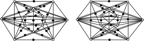
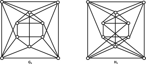
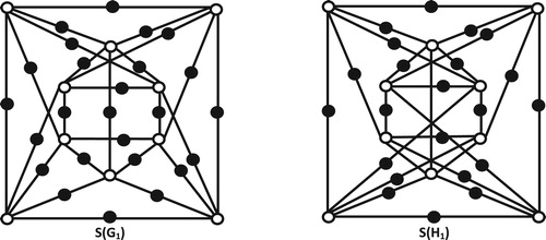
Example 2.1

Applying Theorem 2.5, here we construct two $\mathcal{L}$-cospectral graphs. We consider regular cospectral graphs $G_1$ and $H_1$ [16] as given in Fig. 1.

We also consider the simplest regular graph $K_2$. In Fig. 2 we present subdivision graphs of $G_1$ and $H_1$. Then by Theorems 2.1 and 2.5, $G_1\dot{\vee }{K}_2$ and $H_1\dot{\vee }{K}_2$ are $\mathcal{L}$-cospectral graphs (see Fig. 3). Similarly, graphs $G_1⊻K_2$, $G_1〈\mathrm{v}〉K_2$ and $G_1〈\mathrm{e}〉K_2$ are $\mathcal{L}$-cospectral with graphs $H_1⊻K_2$, $H_1〈\mathrm{v}〉K_2$ and $H_1〈\mathrm{e}〉K_2$ respectively.

Fig. 1 Two cospectral regular graphs.

Fig. 2 Subdivision of $G_1$ and $H_1$.

Fig. 3 Non-regular nonisomorphic $\mathcal{L}$-cospectral graphs $G_1\dot{\vee }{K}_2$ and $H_1\dot{\vee }{K}_2$.

Notes

Peer review under responsibility of Kalasalingam University.

References

- Chung F.R.K. Spectral Graph Theory CBMS. Reg. Conf. Ser. Math. vol. 92 (1997) AMS. providence, RI.
- Banerjee A. Jost J. On the spectrum of the normalized graph Laplacian Linear Algebra Appl. 428 2008 3015 3022
- Butler S. Grout J. A construction of cospectral graphs for the normalized Laplacian Electron. J. Combin. 18 2011 231
- Li H.H. Li J.S. A note on the normalized Laplacian spectra Taiwanese J. Math. 15 2011 129 139
- Harary F. Graph Theory 1969 Addison-Wesley Reading, PA
- Butler S. (Ph.D. dissertation) Eigenvalues and Structures of Graphs 2008 University of California San Diego
- Cvetkovic D. Rowlinson P. Simic S. An Introduction to the Theory of Graph Spectra 2009 Cambridge University Press
- Xie P. Zhang Z. Comellas F. The normalized Laplacian spectrum of subdivisions of a graph Appl. Math. Comput. 286 2016 250 256
- Cvetkovic D.M. Doob M. Sachs H. Spectra of Graphs–Theory and Applications third ed. 1995 Johann Ambrosius Barth Heidelberg
- X.G. Liu, Z.H. Zhang, Spectra of subdivision-vertex and subdivision-edge joins of graphs, (submitted for publication), http://arxiv:1212.0619.
- Liu X. Zhou J. Bu C. Resistance distance and Kirchhoff index of R-vertex join and R-edge join of two graphs Discrete Appl. Math. 187 2015 130 139
- Indulal G. Spectra of two new joins of graphs and infinite families of integral graphs Kragujevac J. Math. 36 2012 133 139
- Godsil C. Royle G. Algebraic Graph Theory 2001 Springer New York
- Cui S.Y. Tian G.X. The spectrum and the signless Laplacian spectrum of coronae Linear Algebra Appl. 437 2012 1692 1703
- McLeman C. McNicholas E. Spectra of coronae Linear Algebra Appl. 435 2011 998 1007
- Vandam E.R. Haemers W.H. Which graphs are determined by their spectrum? Linear Algebra Appl. 373 2003 241 272