Status connectivity indices and co-indices of graphs and its computation to some distance-balanced graphs

Abstract

The status of a vertex $u$, denoted by ${\sigma }_G\left(u\right)$, is the sum of the distances between $u$ and all other vertices in a graph $G$. The first and second status connectivity indices of a graph $G$ are defined as $S_1\left(G\right)={\sum }_{uv\in E\left(G\right)}[{\sigma }_G\left(u\right)+{\sigma }_G\left(v\right)]$ and $S_2\left(G\right)={\sum }_{uv\in E\left(G\right)}{\sigma }_G\left(u\right){\sigma }_G\left(v\right)$ respectively, where $E\left(G\right)$ denotes the edge set of $G$. In this paper we have defined the first and second status co-indices of a graph $G$ as $\overline{S_1}\left(G\right)={\sum }_{uv\notin E\left(G\right)}[{\sigma }_G\left(u\right)+{\sigma }_G\left(v\right)]$ and $\overline{S_2}\left(G\right)={\sum }_{uv\notin E\left(G\right)}{\sigma }_G\left(u\right){\sigma }_G\left(v\right)$ respectively. Relations between status connectivity indices and status co-indices are established. Also these indices are computed for intersection graph, hypercube, Kneser graph and achiral polyhex nanotorus.

Keywords:

• Distance in graph
• Status indices
• Distance-balanced graphs

1 Introduction

The graph theoretic models can be used to study the properties of molecules in theoretical chemistry. The oldest well known graph parameter is the Wiener index which was used to study the chemical properties of paraffins [1]. The Zagreb indices were used to study the structural property models [2,3]. Ramane and Yalnaik [4] obtained the status connectivity indices and analyzed its correlation with the boiling point of benzenoid hydrocarbons. In this paper we define the status co-indices of a graph and establish the relations between the status connectivity indices and status co-indices. Also we obtain the bounds for the status connectivity indices of connected complement graphs. Further we compute these status indices for intersection graph, hypercube, Kneser graph and achiral polyhex nanotorus.

Let $G$ be a connected graph with $n$ vertices and $m$ edges. Let $V\left(G\right)$ be the vertex set of $G$ and $E\left(G\right)$ be an edge set of $G$. The edge joining the vertices $u$ and $v$ is denoted by $uv$. The degree of a vertex $u$ in a graph $G$ is the number of edges incident to $u$ and is denoted by $d_G\left(u\right)$. The distance between the vertices $u$ and $v$ is the length of shortest path joining $u$ and $v$ and is denoted by $d_G(u,v)$. The diameter of $G$ is the maximum distance between all pair of vertices of $G$ and is denoted by $diam\left(G\right)$.

The status (or transmission) of a vertex $u\in V\left(G\right)$, denoted by ${\sigma }_G\left(u\right)$ is defined as [5], $${\sigma }_G\left(u\right)=\sum _{v\in V\left(G\right)}{d}_G(u,v).$$

A connected graph $G$ is self-median if the value ${\sigma }_G\left(u\right)$ is constant for all vertices $u$ of $G$ [6]. A graph $G$ is distance-balanced if for all edges $uv$ of $G$, the following equality holds [7,8], $$\left|\{w\in V\left(G\right)\mid d_G(w,u)<d_G(w,v)\}\right|=\left|\{w\in V\left(G\right)\mid d_G(w,v)<d_G(w,u)\}\right|.$$

Balakrishnan et al. [9] noticed that the concepts of distance-balanced and self-median are the same. A connected graph is distance-balanced if and only if it is self-median.

A connected graph $G$ is said to be $k$-distance-balanced if ${\sigma }_G\left(u\right)=k$ for every vertex $u\in V\left(G\right)$.

The Wiener index $W\left(G\right)$ of a connected graph $G$ is defined as [1], $$W\left(G\right)=\sum _{\{u,v\}\subseteq V\left(G\right)}{d}_G(u,v)=\frac{1}{2}\sum _{u\in V\left(G\right)}{\sigma }_G\left(u\right).$$More results about Wiener index can be found in [10–16].

The first and second Zagreb indices of a graph $G$ are defined as [2] $$M_1\left(G\right)=\sum _{uv\in E\left(G\right)}\left[d_G\left(u\right)+d_G\left(v\right)\right]\mathrm{and}{M}_2\left(G\right)=\sum _{uv\in E\left(G\right)}{d}_G\left(u\right)d_G\left(v\right).$$Results on the Zagreb indices can be found in [17–23].

The first and second Zagreb co-indices of a graph $G$ are defined as [24] $$\overline{M_1}\left(G\right)=\sum _{uv\notin E\left(G\right)}\left[d_G\left(u\right)+d_G\left(v\right)\right]\mathrm{and}\overline{M_2}\left(G\right)=\sum _{uv\notin E\left(G\right)}{d}_G\left(u\right)d_G\left(v\right).$$More results on Zagreb co-indices can be found in [25,26].

The first status connectivity index $S_1\left(G\right)$ and second status connectivity index $S_2\left(G\right)$ of a graph $G$ are defined as [4] (1) $$S_1\left(G\right)=\sum _{uv\in E\left(G\right)}\left[{\sigma }_G\left(u\right)+{\sigma }_G\left(v\right)\right]\mathrm{and}{S}_2\left(G\right)=\sum _{uv\in E\left(G\right)}{\sigma }_G\left(u\right){\sigma }_G\left(v\right).$$(1)

We observe that the first status connectivity index is nothing but the degree distance of a graph introduced by Dobrynin and Kotchetova [27] and Gutman [28]. The degree distance of $G$ is $$D^{\prime }\left(G\right)=\sum _{u\in V\left(G\right)}{d}_G\left(u\right){\sigma }_G\left(u\right)=\sum _{\{u,v\}\subseteq V\left(G\right)}[d_G\left(u\right)+d_G\left(v\right)]d_G(u,v).$$The degree distance of graphs is well studied in the literature [29–36].

Analog to Eq. (1) and the definition of Zagreb co-indices, we define the first status co-index $\overline{S_1}\left(G\right)$ and the second status co-index $\overline{S_2}\left(G\right)$ as $$\overline{S_1}\left(G\right)=\sum _{uv\notin E\left(G\right)}\left[{\sigma }_G\left(u\right)+{\sigma }_G\left(v\right)\right]\mathrm{and}\overline{S_2}\left(G\right)=\sum _{uv\notin E\left(G\right)}\left[{\sigma }_G\left(u\right){\sigma }_G\left(v\right)\right].$$

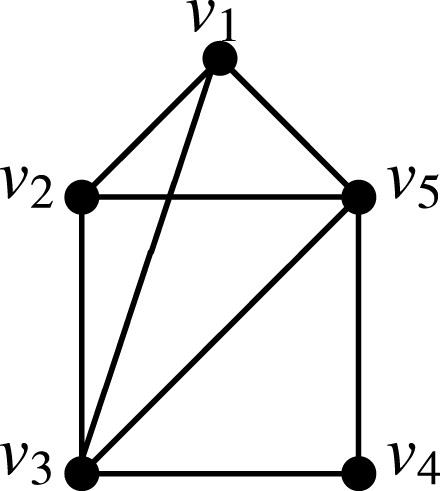
For a graph given in Fig. 1, $S_1=74$, $S_2=169$, $\overline{S_1}=22$ and $\overline{S_2}=60$.

short-legendFig. 1

2 Status connectivity indices and co-indices

In [4] the results on status connectivity indices are obtained. In this section we obtain further results on the status connectivity indices and co-indices of graphs.

Proposition 2.1

Let $G$ be a connected graph on $n$ vertices. Then $$\overline{S_1}\left(G\right)=2(n-1)W\left(G\right)-S_1\left(G\right)$$and $$\overline{S_2}\left(G\right)=2{\left(W\left(G\right)\right)}^2-\frac{1}{2}\sum _{u\in V\left(G\right)}{\left({\sigma }_G\left(u\right)\right)}^2-S_2\left(G\right).$$

Proof

$$\overline{S_1}\left(G\right)=\sum _{uv\notin E\left(G\right)}\left[{\sigma }_G\left(u\right)+{\sigma }_G\left(v\right)\right]$$$$=\sum _{\left\{u,v\right\}\subseteq V\left(G\right)}\left[{\sigma }_G\left(u\right)+{\sigma }_G\left(v\right)\right]-\sum _{uv\in E\left(G\right)}\left[{\sigma }_G\left(u\right)+{\sigma }_G\left(v\right)\right]$$$$=(n-1)\sum _{u\in V\left(G\right)}{\sigma }_G\left(u\right)-S_1\left(G\right)$$$$=2(n-1)W\left(G\right)-S_1\left(G\right).$$Also $$\overline{S_2}\left(G\right)=\sum _{uv\notin E\left(G\right)}\left[{\sigma }_G\left(u\right){\sigma }_G\left(v\right)\right]$$$$=\sum _{\left\{u,v\right\}\subseteq V\left(G\right)}\left[{\sigma }_G\left(u\right){\sigma }_G\left(v\right)\right]-\sum _{uv\in E\left(G\right)}\left[{\sigma }_G\left(u\right){\sigma }_G\left(v\right)\right]$$$$=\frac{1}{2}\left[{\left[\sum _{u\in V\left(G\right)}{\sigma }_G\left(u\right)\right]}^2-\sum _{u\in V\left(G\right)}{\sigma }_G{\left(u\right)}^2\right]-S_2\left(G\right)$$$$=2{\left(W\left(G\right)\right)}^2-\frac{1}{2}\sum _{u\in V\left(G\right)}{\left({\sigma }_G\left(u\right)\right)}^2-S_2\left(G\right).$$

Corollary 2.2

Let $G$ be a connected graph with $n$ vertices, $m$ edges and $diam\left(G\right)\le 2$. Then $$\overline{S_1}\left(G\right)=2n{(n-1)}^2-6m(n-1)+M_1\left(G\right)$$and $$\overline{S_2}\left(G\right)={(n-1)}^2\left[2n(n-1)-8m\right]+2m^2+\left(2n-\frac{5}{2}\right)M_1\left(G\right)-M_2\left(G\right).$$

Proof

For any graph $G$ of $diam\left(G\right)\le 2$, ${\sigma }_G\left(u\right)=2n-2-d_G\left(u\right)$ and $$W\left(G\right)=m+2\left[\frac{n(n-1)}{2}-m\right]=n(n-1)-m.$$Also $S_1\left(G\right)=4m(n-1)-M_1\left(G\right)$ and $S_2\left(G\right)=4m{(n-1)}^2-2(n-1)M_1\left(G\right)+M_2\left(G\right)$ [4]. Therefore by Proposition 2.1, $$\overline{S_1}\left(G\right)=2(n-1)[n(n-1)-m]-\left\{4m(n-1)-M_1\left(G\right)\right\}$$$$=2n{(n-1)}^2-6m(n-1)+M_1\left(G\right)$$and $$\overline{S_2}\left(G\right)=2{\left[n(n-1)-m\right]}^2-\frac{1}{2}\sum _{u\in V\left(G\right)}{(2n-2-d_G\left(u\right))}^2-\left[4m{(n-1)}^2-2(n-1)M_1\left(G\right)+M_2\left(G\right)\right]$$$$=2{\left[n(n-1)-m\right]}^2-\frac{1}{2}\left[\sum _{u\in V\left(G\right)}{(2n-2)}^2-2(2n-2)\sum _{u\in V\left(G\right)}{d}_G\left(u\right)+\sum _{u\in V\left(G\right)}{\left(d_G\left(u\right)\right)}^2\right]$$$$-\left[4m{(n-1)}^2-2(n-1)M_1\left(G\right)+M_2\left(G\right)\right]$$$$=2{\left[n(n-1)-m\right]}^2-\frac{1}{2}\left[n{(2n-2)}^2-4m(2n-2)+M_1\left(G\right)\right]-\left[4m{(n-1)}^2-2(n-1)M_1\left(G\right)+M_2\left(G\right)\right]$$$$={(n-1)}^2\left[2n(n-1)-8m\right]+2m^2+\left(2n-\frac{5}{2}\right)M_1\left(G\right)-M_2\left(G\right).$$

Proposition 2.3

Let $G$ be a connected graph with $n$ vertices, $m$ edges and $diam\left(G\right)\le 2$. Then $$\overline{S_1}\left(G\right)=2(n-1)\left[n(n-1)-2m\right]-\overline{M_1}\left(G\right)$$and $$\overline{S_2}\left(G\right)=2{(n-1)}^2\left[n(n-1)-2m\right]-2(n-1)\overline{M_1}\left(G\right)+\overline{M_2}\left(G\right).$$

Proof

For any graph $G$ of $diam\left(G\right)\le 2$, ${\sigma }_G\left(u\right)=2n-2-d_G\left(u\right)$. Therefore $$\overline{S_1}\left(G\right)=\sum _{uv\notin E\left(G\right)}\left[(2n-2-d_G\left(u\right))+(2n-2-d_G\left(v\right))\right]$$$$=\left[\frac{n(n-1)}{2}-m\right](4n-4)-\sum _{uv\notin E\left(G\right)}\left[d_G\left(u\right)+d_G\left(v\right)\right]$$$$=2(n-1)\left[n(n-1)-2m\right]-\overline{M_1}\left(G\right)$$and $$\overline{S_2}\left(G\right)=\sum _{uv\notin E\left(G\right)}\left[(2n-2-d_G\left(u\right))(2n-2-d_G\left(v\right))\right]$$$$=\left[\frac{n(n-1)}{2}-m\right]{(2n-2)}^2-(2n-2)\sum _{uv\notin E\left(G\right)}\left[d_G\left(u\right)+d_G\left(v\right)\right]+\sum _{uv\notin E\left(G\right)}\left(d_G\left(u\right)d_G\left(v\right)\right)$$$$=2{(n-1)}^2\left[n(n-1)-2m\right]-2(n-1)\overline{M_1}\left(G\right)+\overline{M_2}\left(G\right).$$

Proposition 2.4

Let $G$ be a graph with $n$ vertices and $m$ edges. Let $\overline{G}$ be the complement of $G$ and it is connected. Then $$S_1\left(\overline{G}\right)\ge (n-1)[n(n-1)-2m]+\overline{M_1}\left(G\right)$$and $$S_2\left(\overline{G}\right)\ge {(n-1)}^2\left[\frac{n(n-1)}{2}-m\right]+(n-1)\overline{M_1}\left(G\right)+\overline{M_2}\left(G\right).$$Equality in both cases holds if and only if $diam\left(\overline{G}\right)\le 2$.

Proof

For any vertex $u$ in $\overline{G}$ there are $n-1-d_G\left(u\right)$ vertices which are at distance $1$ and the remaining $d_G\left(u\right)$ vertices are at distance at least $2$. Therefore $${\sigma }_{\overline{G}}\left(u\right)\ge [n-1+d_G\left(u\right)]+2d_G\left(u\right)$$$$=n-1+d_G\left(u\right).$$Therefore, $$S_1\left(\overline{G}\right)=\sum _{uv\in E\left(\overline{G}\right)}\left[{\sigma }_{\overline{G}}\left(u\right)+{\sigma }_{\overline{G}}\left(v\right)\right]$$$$\ge \sum _{uv\in E\left(\overline{G}\right)}\left[n-1+d_G\left(u\right)+n-1+d_G\left(v\right)\right]$$$$=\sum _{uv\notin E\left(G\right)}\left[2n-2+d_G\left(u\right)+d_G\left(v\right)\right]$$$$=\left[\frac{n(n-1)}{2}-m\right](2n-2)+\sum _{uv\notin E\left(G\right)}[d_G\left(u\right)+d_G\left(v\right)]$$$$=[n(n-1)-2m](n-1)+\overline{M_1}\left(G\right).$$And $$S_2\left(\overline{G}\right)=\sum _{uv\in E\left(\overline{G}\right)}{\sigma }_{\overline{G}}\left(u\right){\sigma }_{\overline{G}}\left(v\right)$$$$\ge \sum _{uv\in E\left(\overline{G}\right)}[n-1+d_G\left(u\right)][n-1+d_G\left(v\right)]$$$$=\sum _{uv\notin E\left(G\right)}\left[{(n-1)}^2+(n-1)[d_G\left(u\right)+d_G\left(v\right)]+\left[d_G\left(u\right)d_G\left(v\right)\right]\right]$$$$=\left[\frac{n(n-1)}{2}-m\right]{(n-1)}^2+(n-1)\overline{M_1}\left(G\right)+\overline{M_2}\left(G\right).$$

For equality: If the diameter of $\overline{G}$ is $1$ or $2$ then the equality holds.

Conversely, let $S_1\left(\overline{G}\right)=(n-1)[n(n-1)-2m]+\overline{M_1}\left(G\right)$.

Suppose, $diam\left(\overline{G}\right)\ge 3$, then there exists at least one pair of vertices, say $u_1$ and $u_2$ such that $d_{\overline{G}}(u_1,u_2)\ge 3$.

Therefore ${\sigma }_{\overline{G}}\left(u_1\right)\ge d_{\overline{G}}\left(u_1\right)+3+2(n-2-d_{\overline{G}}\left(u_1\right))=n+d_G\left(u_1\right)$. Similarly ${\sigma }_{\overline{G}}\left(u_2\right)\ge n+d_G\left(u_2\right)$ and for all other vertices $u$ of $\overline{G}$, ${\sigma }_{\overline{G}}\left(u\right)\ge n-1+d_G\left(u\right)$.

Partition the edge set of $\overline{G}$ into three sets $E_1$, $E_2$ and $E_3$, where $$E_1=\left\{u_{1}v\right|{\sigma }_{\overline{G}}\left(u_1\right)\ge n+d_G\left(u_1\right)\text{and}{\sigma }_{\overline{G}}\left(v\right)\ge n-1+d_G\left(v\right)\},$$ $$E_2=\left\{u_{2}v\right|{\sigma }_{\overline{G}}\left(u_2\right)\ge n+d_G\left(u_2\right)\text{and}{\sigma }_{\overline{G}}\left(v\right)\ge n-1+d_G\left(v\right)\}$$and $$E_3=\left\{uv\right|{\sigma }_{\overline{G}}\left(u\right)\ge n-1+d_G\left(u\right)\text{and}{\sigma }_{\overline{G}}\left(v\right)\ge n-1+d_G\left(v\right)\}.$$It is easy to check that $\left|E_1\right|=d_{\overline{G}}\left(u_1\right)$, $\left|E_2\right|=d_{\overline{G}}\left(u_2\right)$ and $\left|E_3\right|=\left(\genfrac{}{}{0ex}{}{n}{2}\right)-m-d_{\overline{G}}\left(u_1\right)-d_{\overline{G}}\left(u_2\right)$.

Therefore $$S_1\left(\overline{G}\right)=\sum _{uv\in E\left(\overline{G}\right)}\left[{\sigma }_{\overline{G}}\left(u\right)+{\sigma }_{\overline{G}}\left(v\right)\right]$$$$=\sum _{uv\in E_1}\left[{\sigma }_{\overline{G}}\left(u\right)+{\sigma }_{\overline{G}}\left(v\right)\right]+\sum _{uv\in E_2}\left[{\sigma }_{\overline{G}}\left(u\right)+{\sigma }_{\overline{G}}\left(v\right)\right]+\sum _{uv\in E_3}\left[{\sigma }_{\overline{G}}\left(u\right)+{\sigma }_{\overline{G}}\left(v\right)\right]$$$$\ge \sum _{uv\in E_1}\left[2n-1+d_G\left(u\right)+d_G\left(v\right)\right]+\sum _{uv\in E_2}\left[2n-1+d_G\left(u\right)+d_G\left(v\right)\right]+\sum _{uv\in E_3}\left[2n-2+d_G\left(u\right)+d_G\left(v\right)\right]$$$$=(2n-1)d_{\overline{G}}\left(u_1\right)+(2n-1)d_{\overline{G}}\left(u_2\right)+(2n-2)\left[\left(\genfrac{}{}{0ex}{}{n}{2}\right)-m-d_{\overline{G}}\left(u_1\right)-d_{\overline{G}}\left(u_2\right)\right]+\sum _{uv\in E\left(\overline{G}\right)}\left[d_G\left(u\right)+d_G\left(v\right)\right]$$$$=(n-1)[n(n-1)-2m]+d_{\overline{G}}\left(u_1\right)+d_{\overline{G}}\left(u_2\right)+\overline{M_1}\left(G\right),$$which is a contradiction. Hence $diam\left(\overline{G}\right)\le 2$.

The equality of $S_2\left(\overline{G}\right)$ can be proved analogously.

3 Status connectivity indices and co-indices of some distance-balanced graphs

A bijection $\alpha$ on $V\left(G\right)$ is called an automorphism of $G$ if it preserves $E\left(G\right)$. In other words, $\alpha$ is an automorphism if for each $u,v\in V\left(G\right)$, $e=uv\in E\left(G\right)$ if and only if $\alpha \left(e\right)=\alpha \left(u\right)\alpha \left(v\right)\in E\left(G\right)$. Let $$Aut\left(G\right)=\{\alpha \mid \alpha :V\left(G\right)⟶V\left(G\right)\text{such that}\alpha \text{and}{\alpha }^{-1}\text{preserve adjacency}\}.$$It is known that $Aut\left(G\right)$ forms a group under the composition of mappings. A graph $G$ is called vertex-transitive if for every two vertices $u$ and $v$ of $G$, there exists an automorphism $\alpha$ of $G$ such that $\alpha \left(u\right)=v$. 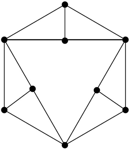It is known that any vertex-transitive graph is vertex degree regular, distance-balanced and self-centered. The graph depicted in Fig. 2 is 14-distance-balanced graph but not degree regular and therefore not vertex-transitive (see [37,38]).

Fig. 2 The distance-balanced but not degree regular graph.

The following lemma is straightforward from the definition of status connectivity indices.

Lemma 3.1

Let $G$ be a connected $k$-distance-balanced graph with $m$ edges. Then $S_1\left(G\right)=2mk$ and $S_2\left(G\right)=m{k}^2.$

Theorem 3.2

[39] Let $G$ be a connected graph on $n$ vertices with the automorphism group $Aut\left(G\right)$ and the vertex set $V\left(G\right)$. Let $V_1,V_2,\dots ,V_t$ be all orbits of the action $Aut\left(G\right)$ on $V\left(G\right)$. Suppose that for each $1\le i\le t$, $k_i$ are the status of vertices in the orbit $V_i$. Then $$W\left(G\right)=\frac{1}{2}\sum _{i=1}^t\left|V_i\right|k_i.$$Specially, if $G$ is vertex-transitive (that is, $t=1$), then $W\left(G\right)=\frac{1}{2}nk$, where $k$ is the status of each vertex of $G$.

Analogous to Theorem 3.2 and as a consequence of Proposition 2.1, we have the following.

Theorem 3.3

Let $G$ be a connected graph on $n$ vertices with the automorphism group $Aut\left(G\right)$ and the vertex set $V\left(G\right)$. Let $V_1,V_2,\dots ,V_t$ be all orbits of the action $Aut\left(G\right)$ on $V\left(G\right)$. Suppose that for each $1\le i\le t$, $d_i$ and $k_i$ are the vertex degree and the status of vertices in the orbit $V_i$, respectively. Then $$S_1\left(G\right)=\sum _{i=1}^t\left|V_i\right|d_i{k}_i\text{and}\overline{S_1}\left(G\right)=(n-1)\sum _{i=1}^t\left[\left|V_i\right|k_i\left(1-\frac{d_i}{n-1}\right)\right].$$Specially, if $G$ is vertex-transitive (that is, $t=1$), then $$S_1\left(G\right)=ndk,S_2\left(G\right)=\frac{1}{2}nd{k}^2,$$ $$\overline{S_1}\left(G\right)=2\left(\genfrac{}{}{0ex}{}{n}{2}\right)k-ndk,\overline{S_2}\left(G\right)=\left[\left(\genfrac{}{}{0ex}{}{n}{2}\right)-\frac{nd}{2}\right]k^2,$$where $d$ and $k$ are the degree and the status of each vertex of $G$ respectively.

The following is a direct consequence of Proposition 2.1, Lemma 3.1 and Theorem 3.2.

Lemma 3.4

Let $G$ be a connected $k$-distance-balanced graph with $m$ edges. Then $$\overline{S_1}\left(G\right)=2\left(\genfrac{}{}{0ex}{}{n}{2}\right)k-2mk\text{and}\overline{S_2}\left(G\right)=\left(\genfrac{}{}{0ex}{}{n}{2}\right)k^2-m{k}^2.$$

Let $S$ be a set and $F=\{S_1,\dots ,S_q\}$ be a non-empty family of distinct non-empty subsets of $S$ such that $S={\bigcup }_{i=1}^q{S}_i$. The intersection graph [40] of $S$ which is denoted by $\Omega \left(F\right)$ has $F$ as its set of vertices and two distinct vertices $S_i$ and $S_j$, $i\ne j$, are adjacent if and only if $S_i\bigcap S_j\ne \varnothing$. Here we will consider a set $S$ of cardinality $p$ and let $F$ be the set of all subsets of $S$ of cardinality $t$, $1<t<p$, which is denoted by $S^{\left\{t\right\}}$. Upon convenience we may set $S=\{1,2,\dots ,p\}$. Let us denote the intersection graph $\Omega \left(S^{\left\{t\right\}}\right)$ by ${\Gamma }^{\left\{t\right\}}=(V,E)$. The number of vertices of this graph is $\left|V\right|=\left(\genfrac{}{}{0ex}{}{p}{t}\right)$ and the degree $d$ of each vertex is as follows: $$d=\left\{\begin{array}{cc}\left(\genfrac{}{}{0ex}{}{p}{t}\right)-\left(\genfrac{}{}{0ex}{}{p-t}{t}\right)-1,\hfill & p\ge 2t\text{;}\hfill \\ \left(\genfrac{}{}{0ex}{}{p}{t}\right)-1,\hfill & p<2t\text{.}\hfill \end{array}\right.$$The number of its edges is as follows: $$\left|E\right|=\left\{\begin{array}{cc}\frac{1}{2}\left(\genfrac{}{}{0ex}{}{p}{t}\right)\left[\left(\genfrac{}{}{0ex}{}{p}{t}\right)-\left(\genfrac{}{}{0ex}{}{p-t}{t}\right)-1\right],\hfill & p\ge 2t\text{;}\hfill \\ \frac{1}{2}\left(\genfrac{}{}{0ex}{}{p}{t}\right)\left[\left(\genfrac{}{}{0ex}{}{p}{t}\right)-1\right],\hfill & p<2t\text{.}\hfill \end{array}\right.$$

Lemma 3.5

[41] The intersection graph ${\Gamma }^{\left\{t\right\}}$ is vertex-transitive and for any $t$-element subset $A$ of $S$ we have $${\sigma }_{{\Gamma }^{\left\{t\right\}}}\left(A\right)=\left\{\begin{array}{cc}\left(\genfrac{}{}{0ex}{}{p}{t}\right)+\left(\genfrac{}{}{0ex}{}{p-t}{t}\right)-1,\hfill & p\ge 2t\text{;}\hfill \\ \left(\genfrac{}{}{0ex}{}{p}{t}\right)-1,\hfill & p<2t\text{.}\hfill \end{array}\right.$$Moreover, $$W\left({\Gamma }^{\left\{t\right\}}\right)=\left\{\begin{array}{cc}\frac{1}{2}\left(\genfrac{}{}{0ex}{}{p}{t}\right)\left(\left(\genfrac{}{}{0ex}{}{p}{t}\right)+\left(\genfrac{}{}{0ex}{}{p-t}{t}\right)-1\right),\hfill & p\ge 2t\text{;}\hfill \\ \frac{1}{2}\left(\genfrac{}{}{0ex}{}{p}{t}\right)\left(\left(\genfrac{}{}{0ex}{}{p}{t}\right)-1\right),\hfill & p<2t\text{.}\hfill \end{array}\right.$$

Theorem 3.6

For intersection graph ${\Gamma }^{\left\{t\right\}}$, $$S_1\left({\Gamma }^{\left\{t\right\}}\right)=\left\{\begin{array}{cc}\left(\genfrac{}{}{0ex}{}{p}{t}\right)\left(\left(\genfrac{}{}{0ex}{}{p}{t}\right)-\left(\genfrac{}{}{0ex}{}{p-t}{t}\right)-1\right)\left(\left(\genfrac{}{}{0ex}{}{p}{t}\right)+\left(\genfrac{}{}{0ex}{}{p-t}{t}\right)-1\right),\hfill & p\ge 2t\text{;}\hfill \\ \left(\genfrac{}{}{0ex}{}{p}{t}\right){\left(\left(\genfrac{}{}{0ex}{}{p}{t}\right)-1\right)}^2,\hfill & p<2t\text{.}\hfill \end{array}\right.$$

$$S_2\left({\Gamma }^{\left\{t\right\}}\right)=\left\{\begin{array}{cc}\frac{1}{2}\left(\genfrac{}{}{0ex}{}{p}{t}\right)\left(\left(\genfrac{}{}{0ex}{}{p}{t}\right)-\left(\genfrac{}{}{0ex}{}{p-t}{t}\right)-1\right){\left(\left(\genfrac{}{}{0ex}{}{p}{t}\right)+\left(\genfrac{}{}{0ex}{}{p-t}{t}\right)-1\right)}^2,\hfill & p\ge 2t\text{;}\hfill \\ \frac{1}{2}\left(\genfrac{}{}{0ex}{}{p}{t}\right){\left(\left(\genfrac{}{}{0ex}{}{p}{t}\right)-1\right)}^3,\hfill & p<2t\text{.}\hfill \end{array}\right.$$

$$\overline{S_1}\left({\Gamma }^{\left\{t\right\}}\right)=\left\{\begin{array}{cc}\left(\genfrac{}{}{0ex}{}{p-t}{t}\right)\left(\genfrac{}{}{0ex}{}{p}{t}\right)\left(\left(\genfrac{}{}{0ex}{}{p}{t}\right)+\left(\genfrac{}{}{0ex}{}{p-t}{t}\right)-1\right),\hfill & p\ge 2t\text{;}\hfill \\ 2\left(\genfrac{}{}{0ex}{}{\left(\genfrac{}{}{0ex}{}{p}{t}\right)}{2}\right)\left(\left(\genfrac{}{}{0ex}{}{p}{t}\right)-1\right)-\left(\genfrac{}{}{0ex}{}{p}{t}\right){\left(\left(\genfrac{}{}{0ex}{}{p}{t}\right)-1\right)}^2,\hfill & p<2t\text{.}\hfill \end{array}\right.$$

$$\overline{S_2}\left({\Gamma }^{\left\{t\right\}}\right)=\left\{\begin{array}{cc}\left[\left(\genfrac{}{}{0ex}{}{\left(\genfrac{}{}{0ex}{}{p}{t}\right)}{2}\right)-\frac{1}{2}\left(\genfrac{}{}{0ex}{}{p}{t}\right)\left(\left(\genfrac{}{}{0ex}{}{p}{t}\right)-\left(\genfrac{}{}{0ex}{}{p-t}{t}\right)-1\right)\right]{\left(\left(\genfrac{}{}{0ex}{}{p}{t}\right)+\left(\genfrac{}{}{0ex}{}{p-t}{t}\right)-1\right)}^2,\hfill & p\ge 2t\text{;}\hfill \\ \left[\left(\genfrac{}{}{0ex}{}{\left(\genfrac{}{}{0ex}{}{p}{t}\right)}{2}\right)-\frac{1}{2}\left(\genfrac{}{}{0ex}{}{p}{t}\right)\left(\left(\genfrac{}{}{0ex}{}{p}{t}\right)-1\right)\right]{\left(\left(\genfrac{}{}{0ex}{}{p}{t}\right)-1\right)}^2,\hfill & p<2t\text{.}\hfill \end{array}\right.$$

Proof

It is a direct consequence of Theorem 3.3 and Lemma 3.5.

The vertex set of the hypercube $H_n$ consists of all $n$-tuples $(b_1,b_2,\dots ,b_n)$ with $b_i\in \{0,1\}$. Two vertices are adjacent if the corresponding tuples differ in precisely one place. Moreover, $H_n$ has exactly $2n$ vertices and $n{2}^{n-1}$ edges. Darafsheh [41] proved that $H_n$ is vertex-transitive and for every vertex $u$, ${\sigma }_{H_n}\left(u\right)=n{2}^{n-1}$. Therefore, by Lemmas 3.1 and 3.4 we have following result.

Theorem 3.7

For hypercube $H_n$, $$S_1\left(G\right)=n^2{2}^{2n-1}\text{and}{S}_2\left(G\right)=n^3{2}^{3n-3},$$ $$\overline{S_1}\left(G\right)=n^2{2}^n(2n-1-2^{n-1})\text{and}\overline{S_2}\left(G\right)=n^3{2}^{2n-2}(2n-1-2^{n-1}).$$

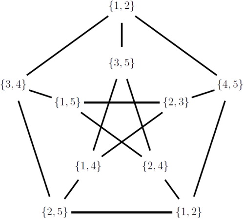
The Kneser graph $K{G}_{p,k}$ is the graph whose vertices correspond to the $k$-element subsets of a set of $p$ elements, and where two vertices are adjacent if and only if the two corresponding sets are disjoint. Clearly we must impose the restriction $p\ge 2k$. The Kneser graph $K{G}_{p,k}$ has $\left(\genfrac{}{}{0ex}{}{p}{k}\right)$ vertices and it is regular of degree $\left(\genfrac{}{}{0ex}{}{p-k}{k}\right)$. Therefore the number of edges of $K{G}_{p,k}$ is $\frac{1}{2}\left(\genfrac{}{}{0ex}{}{p}{k}\right)\left(\genfrac{}{}{0ex}{}{p-k}{k}\right)$ (see [42]). The Kneser graph $K{G}_{n,1}$ is the complete graph on $n$ vertices. The Kneser graph $K{G}_{2p-1,p-1}$ is known as the odd graph $O_p$. The odd graph $O_3=K{G}_{5,2}$ is isomorphic to the Petersen graph (see Fig. 3).

Fig. 3 The odd graph $O_3=K{G}_{5,2}$.

Lemma 3.8

[42] The Kneser graph $K{G}_{p,k}$ is vertex-transitive and for each $k$-subset $A$, ${\sigma }_{K{G}_{p,k}}\left(A\right)=\frac{2W\left(K{G}_{p,k}\right)}{\left(\genfrac{}{}{0ex}{}{p}{k}\right)}$.

Following proposition follows from Lemmas 3.8 and 3.1.

Proposition 3.9

For a Kneser graph $K{G}_{p,k}$ we have $$S_1\left(K{G}_{p,k}\right)=2W\left(K{G}_{p,k}\right)\left(\genfrac{}{}{0ex}{}{p-k}{k}\right)$$and $$S_2\left(K{G}_{p,k}\right)=\left(\genfrac{}{}{0ex}{}{p-k}{k}\right)\left[\frac{2{\left(W\left(K{G}_{p,k}\right)\right)}^2}{\left(\genfrac{}{}{0ex}{}{p}{k}\right)}\right].$$

Following proposition follows from Proposition 2.1, Lemma 3.8 and Proposition 3.9.

Proposition 3.10

For a Kneser graph $K{G}_{p,k}$ we have $$\overline{S_1}\left(K{G}_{p,k}\right)=2W\left(K{G}_{p,k}\right)\left[\left(\genfrac{}{}{0ex}{}{p}{k}\right)-\left(\genfrac{}{}{0ex}{}{p-k}{k}\right)-1\right]$$and $$\overline{S_2}\left(K{G}_{p,k}\right)=2{\left(W\left(K{G}_{p,k}\right)\right)}^2-W\left(K{G}_{p,k}\right)-\left(\genfrac{}{}{0ex}{}{p-k}{k}\right)\left[\frac{2{\left(W\left(K{G}_{p,k}\right)\right)}^2}{\left(\genfrac{}{}{0ex}{}{p}{k}\right)}\right].$$

A nanostructure called achiral polyhex nanotorus (or toroidal fullerenes) of perimeter $p$ and length $q$, denoted by $T[p,q]$ is depicted in Fig. 4 and its 2-dimensional molecular graph is in Fig. 5. It is regular of degree 3 and has $pq$ vertices and $\frac{3pq}{2}$ edges.

Fig. 4 A achiral polyhex nanotorus (or toroidal fullerenes) $T[p,q]$.

Fig. 5 A 2-dimensional lattice for an achiral polyhex nanotorus $T[p,q]$.

The following lemma was proved in [39,43].

Lemma 3.11

[39,43] The achiral polyhex nanotorus $T=T[p,q]$ is vertex-transitive such that for an arbitrary vertex $u\in V\left(T\right)$, $${\sigma }_T\left(u\right)=\left\{\begin{array}{cc}\frac{q}{12}(6p^2+q^2-4),\hfill & q<p\text{;}\hfill \\ \frac{p}{12}(3q^2+3pq+p^2-4),\hfill & q\ge p\text{.}\hfill \end{array}\right.$$

The following is a direct consequence of Lemmas 3.1 and 3.11.

Corollary 3.12

Let $T=T[p,q]$ be a achiral polyhex nanotorus. Then $$S_1\left(T\right)=\left\{\begin{array}{cc}\frac{p{q}^2}{4}(6p^2+q^2-4),\hfill & q<p\text{;}\hfill \\ \frac{p^{2}q}{4}(3q^2+3pq+p^2-4),\hfill & q\ge p\hfill \end{array}\right.$$and $$S_2\left(T\right)=\left\{\begin{array}{cc}\frac{p{q}^3}{96}{(6p^2+q^2-4)}^2,\hfill & q<p\text{;}\hfill \\ \frac{p^{3}q}{96}{(3q^2+3pq+p^2-4)}^2,\hfill & q\ge p\text{.}\hfill \end{array}\right.$$

Corollary 3.13

Let $T=T[p,q]$ be a achiral polyhex nanotorus. Then $$\overline{S_1}\left(T\right)=\left\{\begin{array}{cc}\frac{p{q}^2}{12}(pq-4)(6p^2+q^2-4),\hfill & q<p\text{;}\hfill \\ \frac{p^{2}q}{12}(pq-4)(3q^2+3pq+p^2-4),\hfill & q\ge p\hfill \end{array}\right.$$and $$\overline{S_2}\left(T\right)=\left\{\begin{array}{cc}\frac{p{q}^3}{288}(pq-4){(6p^2+q^2-4)}^2,\hfill & q<p\text{;}\hfill \\ \frac{p^{3}q}{288}(pq-4){(3q^2+3pq+p^2-4)}^2,\hfill & q\ge p\text{.}\hfill \end{array}\right.$$

Proof

Since $2W\left(G\right)={\sum }_{u\in V\left(G\right)}{\sigma }_G\left(u\right)$ and polyhex nanotorus $T[p,q]$ has $pq$ vertices, by Lemma 3.11, the Wiener index of polyhex nanotorus $T[p,q]$ is as follows 43]: $$W\left(T\right)=\left\{\begin{array}{cc}\frac{p{q}^2}{24}(6p^2+q^2-4),\hfill & q<p\text{;}\hfill \\ \frac{p^{2}q}{24}(3q^2+3pq+p^2-4),\hfill & q\ge p\text{.}\hfill \end{array}\right.$$

Substituting this and Corollary 3.12 in Proposition 2.1 we get the results.

Acknowledgments

Authors are thankful to the referees for their suggestions. The first author HSR is thankful to the University Grants Commission (UGC), New Delhi, India for support through grant under UGC-SAP DRS-III, 2016–2021: F.510/3/DRS-III /2016 (SAP-I). The second author ASY is thankful to the University Grants Commission (UGC), New Delhi, India for support through Rajiv Gandhi National Fellowship No. F1-17.1/2014–15/RGNF-2014-15-SC-KAR-74909.

References

- WienerH., Structural determination of paraffin boiling points, J. Am. Chem. Soc., 69 1947 17–20
- GutmanI., TrinajstićN., Graph theory and molecular orbitals. Total π-electron energy of alternant hydrocarbons, Chem. Phys. Lett., 17 1972 535–538
- TodeschiniR., ConsonniV., Handbook of Molecular Descriptors 2000Wiley-VCH Weinheim
- RamaneH.S., YalnaikA.S., Status connectivity indices of graphs and its applications to the boiling point of benzenoid hydrocarbons, J. Appl. Math. Comput., 55 2017 609–627
- HararyF., Status and contrastatus, Sociometry, 22 1959 23–43
- CabelloS., LukšičP., The complexity of obtaining a distance-balanced graph, Electron. J. Combin., 18 2011 Paper 49
- HandaK., Bipartite graphs with balanced (a,b)-partitions, Ars Combin., 51 1999 113–119
- JerebicJ., KlavžarS., RallD.F., Distance-balanced graphs, Ann. Comb., 12 2008 71–79
- BalakrishnanK., ChangatM., PeterinI., ŠpacapanS., ŠparlP., SubhamathiA.R., Strongly distance-balanced graphs and graph products, European J. Combin., 30 2009 1048–1053
- DasK.C., GutmanI., Estimating the Wiener index by means of number of vertices, number of edges and diameter, MATCH Commun. Math. Comput. Chem., 64 2010 647–660
- DobryninA.A., EntringerR., GutmanI., Wiener index of trees: theory and applications, Acta Appl. Math., 66 2001 211–249
- GutmanI., YehY., LeeS., LuoY., Some recent results in the theory of the Wiener number, Indian J. Chem., 32A 1993 651–661
- NikolićS., TrinajstićN., MihalićZ., The Wiener index: development and applications, Croat. Chem. Acta, 68 1995 105–129
- RamaneH.S., ManjalapurV.V., Note on the bounds on Wiener number of a graph, MATCH Commun. Math. Comput. Chem., 76 2016 19–22
- RamaneH.S., RevankarD.S., GanagiA.B., On the Wiener index of a graph, J. Indones. Math. Soc., 18 2012 57–66
- WalikarH.B., ShigehalliV.S., RamaneH.S., Bounds on the Wiener number of a graph, MATCH Commun. Math. Comput. Chem., 50 2004 117–132
- BorovicaninB., DasK.C., FurtulaB., GutmanI., Zagreb indices: bounds and extremal graphs GutmanI., FurtulaB., DasK.C., MilovanovicE., MilovanovicI.Bounds in Chemical Graph Theory - Basics2017Uni. Kragujevac Kragujevac 67–153
- DasK.C., XuK., NamJ., Zagreb indices of graphs, Front. Math. China, 10 2015 567–582
- GutmanI., DasK.C., The first Zagreb index 30 years after, MATCH Commun. Math. Comput. Chem., 50 2004 83–92
- GutmanI., FurtulaB., Kovijanić VukićevićŽ., PopivodaG., On Zagreb indices and coindices, Math. Comput. Chem., 74 2015 5–16
- KhalifehM.H., Yousefi-AzariH., AshrafiA.R., The first and second Zagreb indices of some graph operations, Discrete Appl. Math., 157 2009 804–811
- NikolićS., KovačevićG., MiličevićA., TrinajstićN., The Zagreb indices 30 years after, Croat. Chem. Acta, 76 2003 113–124
- ZhouB., GutmanI., Further properties of Zagreb indices, MATCH Commun. Math. Comput. Chem., 54 2005 233–239
- DošlićT., Vertex-weighted Wiener polynomials for composite graphs, Ars Math. Contemp., 1 2008 66–80
- AshrafiA.R., DošlićT., HamzehA., The Zagreb coindices of graph operations, Discrete Appl. Math., 158 2010 1571–1578
- AshrafiA.R., DošlićT., HamzehA., Extremal graphs with respect to the Zagreb coindices, MATCH Commun. Math. Comput. Chem., 65 2011 85–92
- DobryninA.A., KochetovaA.A., Degree distance of a graph: a degree analogue of the Wiener index, J. Chem. Inf. Comput. Sci., 34 1994 1082–1086
- GutmanI., Selected properties of the Schultz molecular topological index, J. Chem. Inf. Comput. Sci., 34 1994 1087–1089
- BucicovschiO., CioabăS.M., The minimum degree distance of graphs of given order and size, Discrete Appl. Math., 156 2008 3518–3521
- DankelmannP., GutmanI., MurkembiS., SwartH.C., On the degree distance of a graph, Discrete Appl. Math., 157 2009 2773–2777
- DasK.C., SuG., XiongL., Relation between degree distance and Gutman index of graphs, MATCH Commun. Math. Comput. Chem., 76 2016 221–232
- IlićA., StevanovićD., FengL., YuG., DankelmannP., Degree distance of unicyclic and bicyclic graphs, Discrete Appl. Math., 159 2011 779–788
- TomescuA.I., Unicyclic and bicyclic graphs having minimum degree distance, Discrete Appl. Math., 156 2008 125–130
- TomescuI., Some extremal properties of the degree distance of a graph, Discrete Appl. Math., 98 1999 159–163
- TomescuI., Properties of connected graphs having minimum degree distance, Discrete Math., 309 2009 2745–2748
- WangH., KangL., Further properties on the degree distance of graphs, J. Comb. Optim., 31 2016 427–446
- AouchicheM., CaporossiG., HansenP., Variable neighborhood search for extremal graphs, 8. Variations on Graffiti 105, Congr. Numer., 148 2001 129–144
- AouchicheM., HansenP., On a conjecture about the Szeged index, European J. Combin., 31 2010 1662–1666
- AshrafiA.R., Wiener index of nanotubes, toroidal fullerenes and nanostars CataldoF., GraovacA., OriO.The Mathematics and Topology of Fullerenes2011Springer Netherlands Dordrecht 21–38
- HararyF., Graph Theory 1968Addison Wesley Reading
- DarafshehM.R., Computation of topological indices of some graphs, Acta Appl. Math., 110 2010 1225–1235
- MohammadyariR., DarafshehM.R., Topological indices of the Kneser graph KGn,k, Filomat, 26 2012 665–672
- YousefiS., Yousefi-AzariH., AshrafiA.R., KhalifehM.H., Computing Wiener and Szeged indices of an achiral polyhex nanotorus, J. Sci. Univ. Teharan, 33 2008 7–11