An algorithm for generating generalized splines on graphs such as complete graphs, complete bipartite graphs and hypercubes

Abstract

An edge labeled graph is a graph $G$ whose edges are labeled with non-zero ideals of a commutative ring $R$. A Generalized Spline on an edge labeled graph $G$ is a vertex labeling of $G$ by elements of the ring $R$, such that the difference between any two adjacent vertex labels belongs to the ideal corresponding to the edge joining both the vertices. The set of generalized splines forms a subring of the product ring $R^{\left|V\right|}$, with respect to the operations of coordinate-wise addition and multiplication. This ring is known as the generalized spline ring $R_G$, defined on the edge labeled graph $G$, for the commutative ring $R$. We have considered particular graphs such as complete graphs, complete bipartite graphs and hypercubes, labeling the edges with the non-zero ideals of an integral domain $R$ and have identified the generalized spline ring $R_G$ for these graphs. Also, general algorithms have been developed to find these splines for the above mentioned graphs, for any number of vertices and Python code has been written for finding these splines.

Keywords:

• Generalized splines
• Complete graphs
• Hypercubes

1 Introduction

The term spline refers to a class of functions used in data interpolation by mathematicians. The simplest spline is a piecewise polynomial function, defined over a subdivided domain, satisfying certain number of smoothness conditions at the nodes (control points) of the subdivision. These smooth curves find extensive use in interpolating complex curves, CAGD and also generate approximate solutions to differential equations. With the application of the algebraic, geometric and topological techniques, the analytic study of splines got enriched both in terms of understanding and applicability. Spline Theory developed independently in topology and geometry. Billera [1] pioneered the study of algebraic splines, introducing methods from Commutative Algebra [2]. Haas [3], Rose [4] and others [5–7] studied the homological and algebraic properties of splines.

Algebraically, the set of splines over a subdivision of domains was seen to be a subring of the product ring $R\times R\times R...\times R$ ($n$ copies), where $R$ was the ring of polynomials and $n$ denoted number of subdivisions of the domain. Also, it was observed that the above spline ring was a module over the ring of polynomials. Identifying the dimension and finding suitable bases for the free spline modules became an active area of research for many mathematicians, still remaining far from being completely understood [8,9]. Classical splines were piecewise polynomials on polytopes with certain order of smoothness conditions imposed on the boundary faces [10]. Simcha Gilbert, Shira Polster and Julianna Tymoczko [11], expanded the family of objects on which these splines were defined to arbitrary graphs, which they called the generalized splines. Billera and Rose [4] have shown that the spline rings built on the dual graphs of polytopes were equivalent to the generalized spline rings defined on arbitrary graphs [11]. Handschy, Melmick and Reinders [12] have studied the generalized spline modules on cycle graphs over the ring of integers $Z$. They have shown the existence of flow-up basis for the spline modules on cycle graphs, thus proving that these spline modules are free. Bowden and Tymoczko [10] considered the module of generalized splines over the quotient ring $Z∕mZ$, which is not an integral domain. They have shown that over $Z∕mZ$, the minimum generating sets are smaller than expected. In fact, it was proved that over a domain, the module of splines contained a free submodule of rank at least the number of vertices [10]. Handschy, Melmick and Reinders [12] have shown that over a PID the module of splines is free with rank equal to the number of vertices. With these, many interesting properties of the generalized splines were studied, which took into consideration the interplay between the graph theoretic and ring theoretic properties. This opened up the possibility of further exploration in this area, as many open questions were left unanswered in these fields.

We have extended the study further and in this paper, we have addressed the open questions posed by Gilbert, Polster and Tymoczko in [11]. We have constructed nontrivial generalized splines for the special cases, where $G$ is a complete graph, complete bipartite graph and hypercubes. All these graphs find extensive applications in network theory and hence our work is important as it adds to the understanding of the algebraic structures of these graphs. In fact, one of the graphs that we have considered is a $n$-dimensional hypercube, which is used to understand structures like communication signals, computer networks, computer graphics, space, virus, etc. We have developed a general algorithm to express the ring of generalized splines for hypercubes of any dimension $n$ $\ge$ 2, taking into account the bipartite nature [13] and Hamiltonian property of the graph [14]. Also, Python code was developed which calculated the elements of the generalized spline ring $R_G$, for complete graphs and complete bipartite graphs. Throughout our work, we have considered the ring $R$ to be an integral domain and the edge labels as the non-zero ideals of the ring $R$.

2 Results & methods used

2.1 Preliminaries

In this section, we give the formal definition of the generalized spline ring $R_G$, for a graph $G$ over a commutative ring $R$, with the edge labels as the non-zero ideals of the ring $R$, as discussed in [11]. We then give the fundamental results which describe the algebraic structure of the ring $R_G$, along with examples, which are used to construct new generalized splines for the complete graphs, complete bipartite graphs and hypercubes. Throughout the manuscript, we have used the notations of [11], except in some cases which we have mentioned clearly.

The definition of an edge labeled graph is as follows:

2.1.1 Definition

Let $G$ $=$ ($V$, $E$) be a graph. Let $R$ be an arbitrary commutative ring with identity which is also an integral domain and let $S$ denote the set of all non-zero ideals of $R$. Let a function $\alpha$ : $E$ $⟶$ $S$ be an edge labeling of G by the non-zero ideals of R. Given an edge labeling $\alpha$, a vertex labeling p : V $⟶$ R is called a generalized spline if $p_u-p_v$ is in $\alpha \left(e\right)$ for every edge $e=〈uv〉$ in E. Let $R_G$ denote the set of all generalized splines of (G, $\alpha$). Then ${\mathit{R}}_{\mathit{G}}$ is an R-module under the operations of co-ordinate wise addition and scalar multiplication.

The compatibility condition known as “edge conditions” used on the edges are defined as:

2.1.2 Definition

Let G $=$ (V, $\alpha$) be an edge labeled graph. An element p $\in$ ${⨁}_{v\in \mathit{V}}$ R, expressed as

p $=$ ($p_{v_1}$, $p_{v_2}$, $\dots$, $p_{v_n}$) satisfies the edge condition at an edge e $=$ $〈v_i{v}_j〉$ if $p_{v_i}-p_{v_j}$ $\in$ $\alpha$ $\left({\mathit{e}}_{\mathit{ij}}\right)$.

The set of splines with the edge conditions is denoted by ${\mathit{R}}_{\mathit{G},\alpha }$. Each element of ${\mathit{R}}_{\mathit{G},\alpha }$ is called a generalized spline. If the edge labeling is clear, it is denoted as ${\mathit{R}}_{\mathit{G}}$.

We now give the definition of nontrivial generalized spline.

2.1.3 Definition

A nontrivial generalized spline is an element $p$ $\in$ $R_G$, that is not in the principal ideal $R\mathbf{1}$, where 1 is the identity element in $R_G$ defined as $\mathbf{1}=(1,1,\dots ,1)$.

The following theorem [11] shows that ${\mathit{R}}_{\mathit{G}}$ is a ring with unity with the operations of coordinate-wise addition and multiplication.

2.1.4 Theorem

${\mathit{R}}_{\mathit{G}}$ is a ring with unity 1, where ${\mathbf{1}}_v$ $=$ 1 for each vertex $v\in V$.

It is proved [11] that ${\mathit{R}}_{\mathit{G}}$ becomes a module over the ring R with the operation of coordinate-wise addition and scalar multiplication where multiplication by $r\in R$, gives the element $$rp=(r{p}_{v_1},r{p}_{v_2},\dots ,r{p}_{v_n})\in R_G$$

Figs. 1 and 2 (discussed in [11]) are two examples of the ring of generalized splines $R_{C_4}$ and $R_{K_4}$, defined on the 4-cycle $C_4$ and the complete graph $K_4$. Here, R is any commutative ring with unity and (${\alpha }_e$) denotes the ideal generated by the single ring element of $R$.

Fig. 1 Example of a generalized spline on the 4-cycle $C_4$.

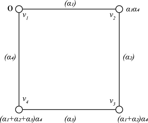
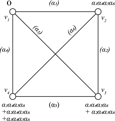
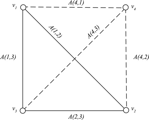
Fig. 2 Example of a generalized spline on the complete graph $K_4$.

Thus, $p$ $=$ ($0$, ${\alpha }_1{\alpha }_4$,(${\alpha }_1$ $+$ ${\alpha }_2$)${\alpha }_4$,(${\alpha }_1$ $+$ ${\alpha }_2+{\alpha }_3$)${\alpha }_4$) $=$ ($p_{v_1}$, $p_{v_2}$, $p_{v_3}$, $p_{v_4}$) represents a generalized spline for $C_4$, because the difference $p_{v_2}-p_{v_1}={\alpha }_1{\alpha }_4$ $\in$ (${\alpha }_1$), and similarly for other adjacent vertices.

Another example giving a generalized spline for the complete graph $K_4$ is given in Fig. 2. Once again, a generalized spline on $K_4$ will be written as $$p=(0,{\alpha }_1{\alpha }_4{\alpha }_5{\alpha }_6,{\alpha }_1{\alpha }_4{\alpha }_5{\alpha }_6+{\alpha }_2{\alpha }_4{\alpha }_5{\alpha }_6,{\alpha }_1{\alpha }_4{\alpha }_5{\alpha }_6+{\alpha }_2{\alpha }_4{\alpha }_5{\alpha }_6+{\alpha }_3{\alpha }_4{\alpha }_5{\alpha }_6)=(p_{v_1},p_{v_2},p_{v_3},p_{v_4},p_{v_5},p_{v_6})$$ which satisfies the edge conditions for all pairs of adjacent vertices. As discussed earlier, the set of generalized splines on an edge labeled graph has a ring structure and $R$-module structure like classical splines. Gilbert, Polster and Tymoczko [11] proved foundational results about the set of generalized splines, completely analyzing the ring of generalized splines for trees. They have obtained the generalized splines for arbitrary cycles and have shown that the study of generalized splines for arbitrary graphs can be reduced to the case of different sub graphs, especially cycles or trees.

Basic problems that arise naturally in the theory of generalized splines is that it focuses on particular examples e.g. a particular choice of the ring $R$, the graph $G$ and the edge labeling function $\alpha$ which maps the edges to the ideals of the ring $R$. Also, the module structure of the ring of generalized splines remains far from being understood in terms of freeness and existence of basis or generating set, for an arbitrary choice of the ring $R$ [11]. However, it is not clear how the ring $R_G$ will be affected under the graph theoretic constructions such as addition or deletion of vertices.

In the rest of the paper, we have extended the study further and addressed the open question posed by Simcha Gilbert, Shira Polster and Juliana Tymoczko in [11]. We have constructed the ring of generalized splines for the special cases, where G is a complete graph $K_n$, complete bipartite graph $K_{n_1,n_2}$ and also for the hypercubes $Q_n$. In all these graphs, the ring $R$ is a commutative ring with identity which is also an integral domain and the edge labels are the non-zero ideals of the ring $R$. Also, the methods of constructing the generalized splines over the complete graphs $K_n$(for any $n$) and complete bipartite graphs $K_{n_1,n_2}$ (for any $n_1$, $n_2$) have been generalized and Python code is developed to write these splines. The bipartite structure and Hamiltonicity of the hypercubes (as defined in [13]) are used to find the general algorithm for writing the set of generalized splines $R_{Q_n}$ (for any $n$).

We discuss the example of generalized spline ring $R_{C_3}$ over the ring of integers for the cycle graph $C_3$ [15].

2.1.5 Example of generalized integer spline on cycle graph $C_3$

Here the generalized integer spline $f$ $=$ ($f_1$, $f_2$, $f_3$) $\in$ $R_{C_3}$, where $C_3$ is a 3-cycle with the edge labels $a_1$, $a_2$, $a_3$ where $a_1$, $a_2$ and $a_3$ are natural numbers (see Fig. 3).

Fig. 3 Example of generalized integer spline on the 3-cycle $C_3$.

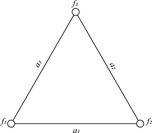
The vertex labels ($f_1$, $f_2$, $f_3$) belonging to $Z$ $\times$ $Z$ $\times$ $Z$ satisfy the following conditions $$f_1\equiv f_{2}mod{a}_1,$$$$f_2\equiv f_{3}mod{a}_2\text{and}$$$$f_3\equiv f_{1}mod{a}_3.$$

We will refer to the preliminaries in the following subsection, throughout the manuscript.

2.2 Important results on $R_G$

Some of the important results for the generalized spline ring $R_G$, relevant to our work are mentioned in this subsection. The first result is theorem 3.8 from [11], which is as follows:

2.2.1 Theorem

Let $C_n$ be a finite edge labeled cycle, given by vertices $v_1$, $v_2$, …, $v_n$ in order. Define the vector $p\in$ $R^{\left|V\right|}$ with $$\left[\begin{array}{c}\hfill p_{v_1}\hfill \\ \hfill p_{v_2}\hfill \\ \hfill p_{v_3}\hfill \\ \hfill ⋮\hfill \\ \hfill ⋮\hfill \\ \hfill ⋮\hfill \\ \hfill p_{v_{n-1}}\hfill \\ \hfill p_{v_n}\hfill \end{array}\right]=p_{v_n}\left[\begin{array}{c}\hfill 1\hfill \\ \hfill 1\hfill \\ \hfill 1\hfill \\ \hfill ⋮\hfill \\ \hfill ⋮\hfill \\ \hfill ⋮\hfill \\ \hfill 1\hfill \\ \hfill 1\hfill \end{array}\right]+{\alpha }_{1,n}\left[\begin{array}{c}\hfill 00\cdots 00\hfill \\ \hfill 10\cdots 00\hfill \\ \hfill 11\cdots 00\hfill \\ \hfill ⋮⋮\cdots ⋮⋮\hfill \\ \hfill ⋮⋮\cdots ⋮⋮\hfill \\ \hfill ⋮⋮\cdots ⋮⋮\hfill \\ \hfill 11\cdots 10\hfill \\ \hfill 11\cdots 11\hfill \end{array}\right]=\left[\begin{array}{c}\hfill {\alpha }_{1,2}\hfill \\ \hfill {\alpha }_{2,3}\hfill \\ \hfill {\alpha }_{3,4}\hfill \\ \hfill ⋮\hfill \\ \hfill ⋮\hfill \\ \hfill ⋮\hfill \\ \hfill {\alpha }_{n-2,n-1}\hfill \\ \hfill {\alpha }_{n-1,n}\hfill \end{array}\right]$$

With arbitrary choices of $p_{v_1}$ $\in$ $R$, ${\alpha }_{i,i+1}$ $\in$ $\alpha \left(e_{i,i+1}\right)$, and ${\alpha }_{1,n}$ $\in$ $\alpha$ $\left(e_{1,n}\right)$. Then $p$ is a generalized spline for $C_n$. The spline $p$ is nontrivial exactly when ${\alpha }_{1,n}$ and at least one of the ${\alpha }_{i,i+1}$ are non-zero.

We have used the following results (corollaries 5.4 and 5.6 from [11]) in proving our results and in obtaining the nontrivial generalized splines for the graphs that we have considered.

2.2.2 Corollary

If $G$ contains any subgraph $G^{\prime }$ for which $R_{G^{\prime }}$ contains a nontrivial generalized spline, then $R_G$ also contains a nontrivial generalized spline.

2.2.3 Corollary

Let $R$ be an integral domain. If the graph $G$ contains at least two vertices, then $R_G$ contains a nontrivial generalized spline.

We will be using the following result for the cycle graph $C_3$, which is also the complete graph $K_3$ (Theorem 3.8 [11]) to identify the ring $R_G$, for the complete graph $K_n$, for $n$ $\ge$ 3.

2.3 Generalized splines for complete graphs, $K_n$,n $\ge$ 3

First we construct nontrivial generalized splines for complete graph $K_3$ [Fig. 4]. Here the edges ($v_1$, $v_2$), ($v_2$, $v_3$) and ($v_3$, $v_1$) of the graph $K_3$ are labeled with the non-zero ideals $A(1,2)$, $A(2,3)$ and $A(3,1)$ respectively of the ring $R$, when $R$ is an integral domain.

Fig. 4 Generalized spline on $K_3$.

It follows from Theorem 3.8 in [11], a generalized spline $p_{K_3}$ on the complete graph $K_3$ is $$p_{K_3}=\left[\begin{array}{c}\hfill 0\hfill \\ \hfill \alpha (1,2)\alpha (1,3)\hfill \\ \hfill (\alpha (1,2)+\alpha (2,3))\alpha (1,3)\hfill \end{array}\right]=\left[\begin{array}{c}\hfill p_{v_1}\hfill \\ \hfill p_{v_2}\hfill \\ \hfill p_{v_3}\hfill \end{array}\right]$$

Here we see that $p_{K_3}$ satisfies the edge conditions on $K_3$, because if the vertices $v_i$ and $v_j$ are adjacent, then $p_{v_i}-p_{v_j}$ $\in$ $A(i,j)$, as $\alpha (i,j)$ is a factor of $p_{v_i}-p_{v_j}$. Here $\alpha (i,j)$ represents any element of the edge ideal $A(i,j)$.

Let $R_{K_3}$ denote the set of all generalized splines of ($K_3$, $\alpha$).

Since $R$ is an integral domain and each $\alpha (i,j)$ is not equal to zero, $R_{K_3}$ contains non-trivial generalized splines.

Using the above result, we have generated the algorithm for developing the generalized spline for the complete graph $K_n$, for any $n\ge 4$.

Also, we will be using the edge conditions (Section 2.1.2) to identify the ring $R_G$, where graph $G$ is complete bipartite graph $K_{n_1,n_2}$, for any $n_1$ and $n_2$.

2.4 Generalized splines for complete bipartite graphs, $K_{n_1,n_2}$

We have generated the algorithm for developing the generalized spline for the complete bipartite graphs with the vertex sets $V_1$ containing $n_1$ vertices and $V_2$ containing $n_2$ vertices. We have used similar notations as above, where we denote the edge ideal corresponding to the edge joining the $i$th and $j$th vertices by $A(i,j)$ and $\alpha (i,j)$ represents an element of the non-zero ideal $A(i,j)$.

We will be using the edge conditions (Section 2.1.2) to identify the ring $R_G$, where graph $G$ is hypercube $Q_n$, for $n\ge 2$.

2.5 Hypercubes

We have extended the method of writing algorithm for the generalized splines to hypercubes, $Q_n$, for $n\ge$ 2 in Section 3.5. Hypercubes, denoted by $Q_n$, are graphs which find extensive use in coding theory in Computer Science and other areas of Mathematics.

3 Results & discussions

3.1 Complete graphs

In this section, we extend the method of constructing the ring of generalized splines $R_{K_n}$, for any $n\ge 4$ starting with the ring $R_{K_3}$ for the complete graph $K_3$ (Section 2.3). In order to get the graph $K_n$, we add a new vertex to the graph $K_{n-1}$ and join the new vertex to the existing $n-1$ vertices in $K_{n-1}$. In the following constructions we consider the ring $R$ to be a commutative ring with identity and also an integral domain. First we construct the graph $K_4$ from the graph $K_3$ and obtain the set of generalized splines $R_{K_4}$ from the ring $R_{K_3}$.

3.1.1 Complete graph ($K_4$), $n$ $=$ 4

We add the vertex $v_4$ to $K_3$ (Fig. 4) and join the new vertex $v_4$ with the vertices $v_1$, $v_2$, $v_3$ of $K_3$ (Fig. 5). The new edges are labeled with the non-zero ideals $A(4,1)$, $A(4,2)$, $A(4,3)$ of integral domain $R$ and $\alpha (4,1)$, $\alpha (4,2)$, $\alpha (4,3)$ are the elements of the respective edge ideals. It can be seen that every vertex label for $p_{K_3}$ $\in$ $R_{K_3}$ (Section 2.3) is multiplied by the factor $\alpha (4,1)\alpha (4,2)\alpha (4,3)$ to get the corresponding vertex labels for the spline $p_{K_4}$ $\in$ $R_{K_4}$, where $R_{K_4}$ denotes the set of all generalized splines for the edge labeled graph ($K_4$, $\alpha$). It is easily verified that if the new vertex $v_4$ is labeled with $p_{v_4}$ $=$ $\alpha (4,1)\alpha (4,2)\alpha (4,3)$, then $p_{K_4}$ becomes a generalized spline for $R_{K_4}$ since the edge conditions are satisfied for the adjacent vertices in $K_4$. So we have $$p_{K_4}=\left[\begin{array}{c}\hfill 0\hfill \\ \hfill \alpha (1,2)\alpha (1,3)〈\alpha (4,1)\alpha (4,2)\alpha (4,3)〉\hfill \\ \hfill (\alpha (1,2)+\alpha (2,3))\alpha (1,3)〈\alpha (4,1)\alpha (4,2)\alpha (4,3)〉\hfill \\ \hfill 〈\alpha (4,1)\alpha (4,2)\alpha (4,3)〉\hfill \end{array}\right]=\left[\begin{array}{c}\hfill p_{v_1}\hfill \\ \hfill p_{v_2}\hfill \\ \hfill p_{v_3}\hfill \\ \hfill p_{v_4}\hfill \end{array}\right]$$

Fig. 5 Generalized spline on $K_4$.

$p_{v_1}-p_{v_2}$ $\in$ $A(1,2)$, since $\alpha (1,2)\in A(1,2)$ is a factor of $p_{v_1}-p_{v_2}$.

Similarly we have $$p_{v_1}-p_{v_3}\in A(1,3),\text{since}\alpha (1,3)\text{is a factor of}{p}_{v_1}-p_{v_3}$$$$p_{v_2}-p_{v_3}\in A(2,3),\text{since}\alpha (2,3)\text{is a factor of}{p}_{v_2}-p_{v_3}$$$$p_{v_4}-p_{v_1}\in A(4,1),\text{since}\alpha (4,1)\text{is a factor of}{p}_{v_4}-p_{v_1}$$$$p_{v_4}-p_{v_2}\in A(4,2),\text{since}\alpha (4,2)\text{is a factor of}{p}_{v_4}-p_{v_2}$$$$p_{v_4}-p_{v_3}\in A(4,3),\text{since}\alpha (4,3)\text{is a factor of}{p}_{v_4}-p_{v_3}$$

Here $p_{v_4}$ $=$ $\alpha (4,1)\alpha (4,2)\alpha (4,3)$ is non-zero because $R$ is an integral domain. Also since $K_3$ is a sub-graph of $K_4$ and $R_{K_3}$ contains nontrivial generalized splines (Sections 2.2.2, 2.2.3) $R_{K_4}$ also contains nontrivial generalized splines.

Using similar methods, we can identify the ring of generalized splines for the complete graph $K_5$.

[cvskip-5pt]

3.1.2 Complete graph ($K_5$), $n$ $=$ 5

We can get $K_5$ by adding the vertex $v_5$ to $K_4$ and the four edges joining $v_5$ to the four vertices $v_1$, $v_2$, $v_3$, $v_4$ of $K_4$ (Fig. 6).

Fig. 6 Generalized spline on $K_5$.

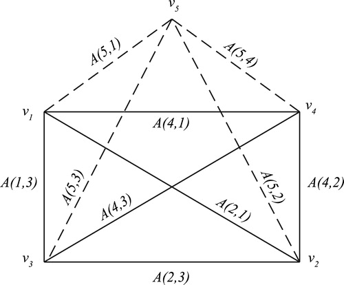
Then in order to get any element of $R_{K_5}$, we multiply each element of $R_{K_4}$ by $\alpha$(5, 1)$\alpha$(5, 2)$\alpha$(5, 3)$\alpha$(5, 4) and label the added vertex $v_5$ with the element $\alpha$(5, 1)$\alpha$(5, 2)$\alpha$(5, 3)$\alpha$(5, 4) $\in$ $R$.

Then any element of $R_{K_5}$ will be of the form: $$p_{K_5}=\left[\begin{array}{c}\hfill 0\hfill \\ \hfill \alpha (1,2)\alpha (1,3)〈\alpha (4,1)\alpha (4,2)\alpha (4,3)〉〈\alpha (5,1)\alpha (5,2)\alpha (5,3)\alpha (5,4)〉\hfill \\ \hfill (\alpha (1,2)+\alpha (2,3))\alpha (1,3)〈\alpha (4,1)\dots \alpha (4,3)〉〈\alpha (5,1)\alpha (5,2)\alpha (5,3)\alpha (5,4)〉\hfill \\ \hfill 〈\alpha (4,1)\alpha (4,2)\alpha (4,3)〉〈\alpha (5,1)\alpha (5,2)\alpha (5,3)\alpha (5,4)〉\hfill \\ \hfill 〈\alpha (5,1)\alpha (5,2)\alpha (5,3)\alpha (5,4)〉\hfill \end{array}\right]=\left[\begin{array}{c}\hfill p_{v_1}\hfill \\ \hfill p_{v_2}\hfill \\ \hfill p_{v_3}\hfill \\ \hfill p_{v_4}\hfill \\ \hfill p_{v_5}\hfill \end{array}\right]$$

Now, we give the algorithm for writing the generalized spline for complete graph $K_n$, for any $n$.

3.1.3 Theorem

We obtain the complete graph $K_n$ by adding the $n\mathrm{th}$ vertex $v_n$ and the edges ($v_n$, $v_1$ ), ($v_n$, $v_2$ ), …, ($v_n$, $v_{n-1}$ ) to the complete graph $K_{n-1}$. Labeling the new edges with the ideals $A(n,1),A(n,2),\dots ,A(n,n-1)$, we get the generalized spline ring $R_{K_n}$, with the elements of the type: $$p_{K_n}=\left[\begin{array}{c}\hfill 0\hfill \\ \hfill \alpha (1,2)\alpha (1,3)〈N_4〉\dots 〈N_n〉\hfill \\ \hfill (\alpha (1,2)+\alpha (2,3))\alpha (1,3)〈N_4〉\dots 〈N_n〉\hfill \\ \hfill 〈N_4〉\dots 〈N_n〉\hfill \\ \hfill 〈N_5〉\dots 〈N_n〉\hfill \\ \hfill ⋮\hfill \\ \hfill ⋮\hfill \\ \hfill ⋮\hfill \\ \hfill 〈N_n〉\hfill \end{array}\right]=\left[\begin{array}{c}\hfill p_{v_1}\hfill \\ \hfill p_{v_2}\hfill \\ \hfill p_{v_3}\hfill \\ \hfill p_{v_4}\hfill \\ \hfill p_{v_5}\hfill \\ \hfill ⋮\hfill \\ \hfill ⋮\hfill \\ \hfill ⋮\hfill \\ \hfill p_{v_n}\hfill \end{array}\right]$$

Here, the notations $N_4$, $N_5$, …, $N_n$ are as follows: $$\begin{array}{c}{N}_4=\alpha (4,1)\alpha (4,2)\alpha (4,3)\hfill \\ N_5=\alpha (5,1)\alpha (5,2)\alpha (5,3)\alpha (5,4)\hfill \\ ⋮\hfill \\ ⋮\hfill \\ ⋮\hfill \\ N_n=\alpha (n,1)\alpha (n,2)\dots \alpha (n,n-1)\hfill \end{array}$$

Proof

We use mathematical induction to prove the algorithm. Let the number of vertices in $K_n$ be $n$. For $n$ $=$ 3, $K_3$ is a cycle graph and it has already been proved in [11] that a generalized spline on $K_3$ is of the form: $$p_{K_3}=\left[\begin{array}{c}\hfill 0\hfill \\ \hfill \alpha (1,2)\alpha (1,3)\hfill \\ \hfill (\alpha (1,2)+\alpha (2,3))\alpha (1,3)\hfill \end{array}\right]=\left[\begin{array}{c}\hfill p_{v_1}\hfill \\ \hfill p_{v_2}\hfill \\ \hfill p_{v_3}\hfill \end{array}\right]$$

As discussed before, we get the generalized spline $p_{K_4}$ for the complete graph $K_4$ by adding one vertex and three edges to $K_3$. The ring of generalized splines $R_{K_4}$ will have elements of the type: $$p_{K_4}=\left[\begin{array}{c}\hfill 0\hfill \\ \hfill \alpha (1,2)\alpha (1,3)〈\alpha (4,1)\alpha (4,2)\alpha (4,3)〉\hfill \\ \hfill (\alpha (1,2)+\alpha (2,3))\alpha (1,3)〈\alpha (4,1)\alpha (4,2)\alpha (4,3)〉\hfill \\ \hfill 〈\alpha (4,1)\alpha (4,2)\alpha (4,3)〉\hfill \end{array}\right]=\left[\begin{array}{c}\hfill p_{v_1}\hfill \\ \hfill p_{v_2}\hfill \\ \hfill p_{v_3}\hfill \\ \hfill p_{v_4}\hfill \end{array}\right]$$

Clearly, the difference $p_{v_i}-p_{v_j}$ of adjacent vertices $v_i$ and $v_j$ is a multiple of $\alpha (i,j)\in A(i,j)$, where $A(i,j)$ is the edge label for the edge joining $v_i$ and $v_j$. We conclude that $p_{K_4}$ satisfies the edge condition for generalized spline over the graph $K_4$.

Inductive step: Assume that there exists a generalized spline $p_{K_{n-1}}$ for the complete graph $K_{n-1}$. Then we have generalized spline $p_{K_{n-1}}$ defined as: $$p_{K_{n-1}}=\left[\begin{array}{c}\hfill 0\hfill \\ \hfill \alpha (1,2)\alpha (1,3)〈N_4〉\dots 〈N_{n-1}〉\hfill \\ \hfill (\alpha (1,2)+\alpha (2,3))\alpha (1,3)〈N_4〉\dots 〈N_{n-1}〉\hfill \\ \hfill 〈N_4〉\dots 〈N_{n-1}〉\hfill \\ \hfill 〈N_5〉\dots 〈N_{n-1}〉\hfill \\ \hfill ⋮\hfill \\ \hfill ⋮\hfill \\ \hfill ⋮\hfill \\ \hfill 〈N_{n-1}〉\hfill \end{array}\right]=\left[\begin{array}{c}\hfill p_{v_1}\hfill \\ \hfill p_{v_2}\hfill \\ \hfill p_{v_3}\hfill \\ \hfill p_{v_4}\hfill \\ \hfill p_{v_5}\hfill \\ \hfill ⋮\hfill \\ \hfill ⋮\hfill \\ \hfill ⋮\hfill \\ \hfill p_{v_{n-1}}\hfill \end{array}\right]$$where $N_4$, $N_5$, …, $N_{n-1}$ are defined as: $$\begin{array}{c}{N}_4=\alpha (4,1)\alpha (4,2)\alpha (4,3)\hfill \\ N_5=\alpha (5,1)\alpha (5,2)\alpha (5,3)\alpha (5,4)\hfill \\ ⋮\hfill \\ ⋮\hfill \\ ⋮\hfill \\ N_{n-1}=\alpha (n-1,1)\alpha (n-1,2)\dots \alpha (n-1,n-2)\hfill \end{array}$$

Let the vertex ‘$v_n$’ and the new edges joining the vertex $v_n$ to the remaining $(n-1)$ vertices be added to $K_{n-1}$ to obtain the complete graph $K_n$. Let the edge labels of the newly added edges be the ideals $A(n,1),A(n,2),\dots ,A(n,n-1)$ of the ring $R$.

Taking the $n$th vertex label as $p_{v_n}$ $=$ $\alpha (n,1)\alpha (n,2)....\alpha (n,n-1)$ $=$ $N_n$, where $\alpha (n,j)\in A(n,j)$, for $j=1,2,\dots .,n-1$ and multiplying each vertex label of the generalized spline for $K_{n-1}$ by $N_n$, we get the generalized spline $p_{K_n}$ for $K_n$ as: $$p_{K_n}=\left[\begin{array}{c}\hfill 0\hfill \\ \hfill \alpha (1,2)\alpha (1,3)〈N_4〉〈N_5〉\dots 〈N_n〉\hfill \\ \hfill (\alpha (1,2)+\alpha (2,3))\alpha (1,3)〈N_4〉〈N_5〉\dots 〈N_n〉\hfill \\ \hfill 〈N_4〉〈N_5〉\dots 〈N_n〉\hfill \\ \hfill 〈N_5〉〈N_6〉\dots 〈N_n〉\hfill \\ \hfill ⋮\hfill \\ \hfill ⋮\hfill \\ \hfill ⋮\hfill \\ \hfill 〈N_n〉\hfill \end{array}\right]$$where $N_n$ $=$ $\alpha (n,1)\alpha (n,2)\dots \alpha (n,n-1)$ is the vertex label for the new vertex $v_n$.

Here we can see the difference between the vertex labels of the vertices $v_n$ and any of the remaining $n-1$ vertices of $K_{n-1}$ is a multiple of $\alpha (n,j)\in A(n,j)$, for $j=1,2,\dots .,n-1$.

Hence, we conclude that $p_{K_n}$ satisfies the edge conditions for the generalized spline for $K_n$.

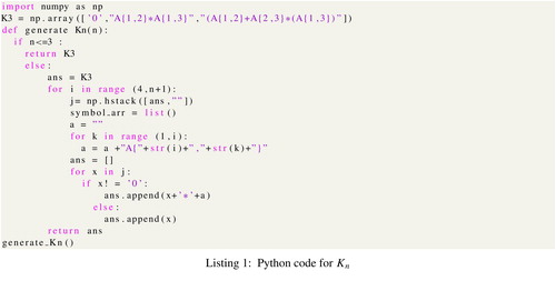
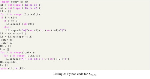
3.1.4 Python code for $K_n$

The Python code is given as

Next we discuss the complete bipartite graphs.

3.2 Complete bipartite graphs ($K_{n_1,n_2}$)

Let $K_{n_1,n_2}$ ($V_1$, $V_2$, $E$) be a complete bipartite graph with vertices partitioned into two disjoint sets $V_1$ and $V_2$, consisting of $n_1$ and $n_2$ vertices respectively. Let $R$ be a commutative ring with unity which is an integral domain and let $S$ denote the set of all non-zero ideals of $R$.

We now extend our method to develop an algorithm for the elements of the generalized spline ring $R_{K_{n_1,n_2}}$, for the complete bipartite graph $K_{n_1,n_2}$. We consider the simple cases for $n_1$, $n_2$ $=$ 1, 2 and 3. The vertices are ordered in the clockwise sense, starting with the first left hand side vertex in the set $V_1$ as the initial vertex.

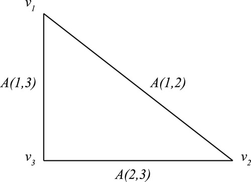
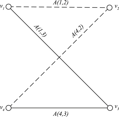
3.2.1 Complete bipartite graph $K_{1,2}$ or $K_{2,1}$

It can be easily seen that $p$ constructed in each of the following situations is a generalized spline since the edge conditions are satisfied by the vertex labels of the adjacent vertices (see Fig. 7). $$p_{K_{1,2}}=\left[\begin{array}{c}\hfill 0\hfill \\ \hfill \alpha (1,2)\hfill \\ \hfill \alpha (1,3)\hfill \end{array}\right]=\left[\begin{array}{c}\hfill p_{v_1}\hfill \\ \hfill p_{v_2}\hfill \\ \hfill p_{v_3}\hfill \end{array}\right]$$ $$p_{K_{2,1}}=\left[\begin{array}{c}\hfill 0\hfill \\ \hfill \alpha (1,2)\alpha (2,3)\hfill \\ \hfill 0\hfill \end{array}\right]=\left[\begin{array}{c}\hfill p_{v_1}\hfill \\ \hfill p_{v_2}\hfill \\ \hfill p_{v_3}\hfill \end{array}\right]$$

Fig. 7 Generalized splines on$K_{1,2}$ and $K_{2,1}$.

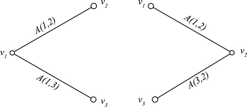
Here the spline $p_{K_{1,2}}$ is nontrivial since $\alpha$(1,2) and $\alpha$(1,3) are non-zero and also the spline $p_{K_{2,1}}$ is nontrivial since $R$ is an integral domain.

3.2.2 Complete bipartite graph $K_{2,2}$

With the clockwise ordering of the vertices, we have the generalized spline for the complete bipartite graph $K_{2,2}$ as follows (see Fig. 8): $$p_{K_{2,2}}=\left[\begin{array}{c}\hfill 0\hfill \\ \hfill \alpha (1,2)〈\alpha (4,2)\alpha (4,3)〉\hfill \\ \hfill \alpha (1,3)〈\alpha (4,2)\alpha (4,3)〉\hfill \\ \hfill 0\hfill \end{array}\right]=\left[\begin{array}{c}\hfill p_{v_1}\hfill \\ \hfill p_{v_2}\hfill \\ \hfill p_{v_3}\hfill \\ \hfill p_{v_4}\hfill \end{array}\right]$$Also, since $K_{1,2}$ or $K_{2,1}$ is a sub graph of $K_{2,2}$ and $R_{K_{1,2}}$, $R_{K_{2,1}}$ contain nontrivial generalized splines (refer Sections 2.2.2, 2.2.3) $R_{K_{2,2}}$ also contains nontrivial generalized splines. It can be easily seen that the edge conditions are satisfied by the vertex labels of the adjacent vertices.

Fig. 8 Generalized spline on $K_{2,2}$.

Now we give the generalized spline for the complete bipartite graph $K_{3,3}$ as follows (Fig. 9):

Fig. 9 Generalized spline on $K_{3,3}$.

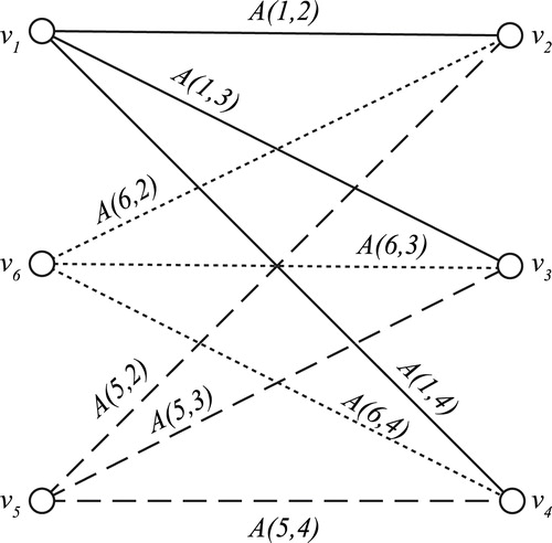
Fig. 10 Generalized spline on $K_{n_1,n_2}$.

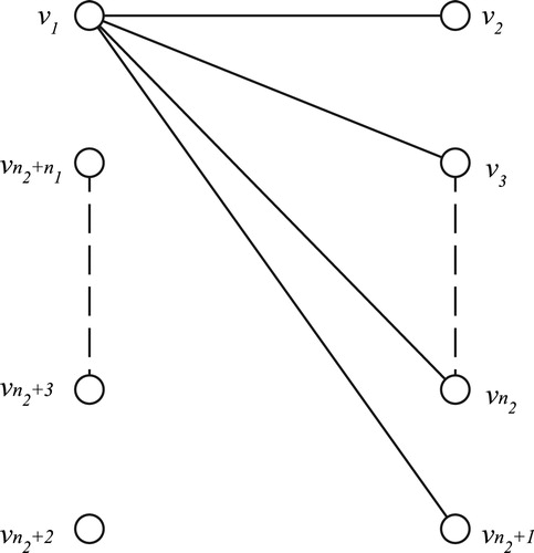
Fig. 11 Hypercubes $Q_1$, $Q_2$ and $Q_3$.

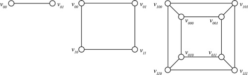
Fig. 12 Hamiltonicity of hypercubes $Q_2$ and $Q_3$.

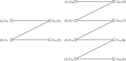
Fig. 13 Bipartite structure of Hypercubes $Q_2$ and $Q_3$.

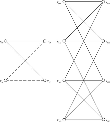
Fig. 14 Graph of Hypercube $Q_4$.

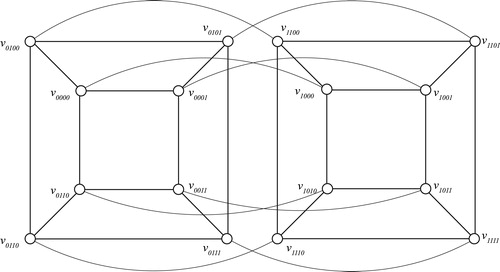
Fig. 15 Bipartite structure and Hamiltonicity of Hypercube $Q_4$.

3.3 Complete bipartite graph $K_{3,3}$

We define $N_5$ and $N_6$ as $$N_5=\alpha (5,2)\alpha (5,3)\alpha (5,4)$$$$N_6=\alpha (6,2)\alpha (6,3)\alpha (6,4)$$ $$p_{K_{3,3}}=\left[\begin{array}{c}\hfill 0\hfill \\ \hfill \alpha (1,2)〈N_5〉〈N_6〉\hfill \\ \hfill \alpha (1,3)〈N_5〉〈N_6〉\hfill \\ \hfill \alpha (1,4)〈N_5〉〈N_6〉\hfill \\ \hfill 0\hfill \\ \hfill 0\hfill \end{array}\right]=\left[\begin{array}{c}\hfill p_{v_1}\hfill \\ \hfill p_{v_2}\hfill \\ \hfill p_{v_3}\hfill \\ \hfill p_{v_4}\hfill \\ \hfill p_{v_5}\hfill \\ \hfill p_{v_6}\hfill \end{array}\right]$$ Next, we consider the general case of complete bipartite graph, where the vertex sets $V_1$ and $V_2$ contain $n_1$ and $n_2$ vertices respectively (see Fig. 10). Here we introduce the notation $$N_{n_2+i}=\alpha (n_2+i,2)\alpha (n_2+i,3)\dots \alpha (n_2+i,n_2+1)\text{for}i=2,3,\dots ,n_1$$

3.3.1 Theorem

Let $K_{n_1,n_2}$ be a complete bipartite graph with vertices partitioned into two disjoint sets $V_1$ and $V_2$, consisting of $n_1$ and $n_2$ vertices respectively (Fig. 10). Then, ordering the vertices in clockwise sense as before, the following $p_{K_{n_1,n_2}}$ gives a generalized spline for the complete bipartite graph $K_{n_1,n_2}$. $$p_{K_{n_1,n_2}}=\left[\begin{array}{c}\hfill 0\hfill \\ \hfill \alpha (1,2)〈N_{(n_2+2)}〉〈N_{(n_2+3)}〉\dots 〈N_{(n_2+n_1)}〉\hfill \\ \hfill \alpha (1,3)〈N_{(n_2+2)}〉〈N_{(n_2+3)}〉\dots 〈N_{(n_2+n_1)}〉\hfill \\ \hfill ⋮\hfill \\ \hfill ⋮\hfill \\ \hfill \alpha (1,n_2+1)〈N_{(n_2+2)}〉〈N_{(n_2+3)}〉\dots 〈N_{(n_2+n_1)}〉\hfill \\ \hfill 0\hfill \\ \hfill ⋮\hfill \\ \hfill ⋮\hfill \\ \hfill 0\hfill \end{array}\right]=\left[\begin{array}{c}\hfill p_{v_1}\hfill \\ \hfill p_{v_2}\hfill \\ \hfill p_{v_3}\hfill \\ \hfill ⋮\hfill \\ \hfill ⋮\hfill \\ \hfill p_{v_{n_2+1}}\hfill \\ \hfill ⋮\hfill \\ \hfill ⋮\hfill \\ \hfill ⋮\hfill \\ \hfill p_{v_{n_2+n_1}}\hfill \end{array}\right]$$ where $N_{n_2+i}=\alpha (n_2+i,2)$ $\alpha (n_2+i,3)$ $\dots$ $\alpha (n_2+i,n_2+1)$, for $i$ $=$ 2,3, $\dots$, $n_1$.

Proof

The proof of the above theorem follows from the observation that the difference of the vertex labels of adjacent vertices is a multiple of the elements belonging to the corresponding edge ideals. However, we note that the algorithm for generating a generalized spline for any complete bipartite graph holds only for the particular ordering of the vertices in the clockwise sense.

Here $N_{n_2+i}=\alpha (n_2+i,2)$ $\alpha (n_2+i,3)$ $\dots$ $\alpha (n_2+i,n_2+1)$,for $i=2,3,\dots ,n_1$ is non-zero since $R$ is an integral domain. Also since $K_{n_1-1,n_2-1}$ is sub graph of $K_{n_1,n_2}$ and $R_{K_{n_1-1,n_2-1}}$ contains nontrivial generalized splines, $R_{K_{n_1,n_2}}$ also contains nontrivial generalized splines.

Here we give the software code for the above algorithm using Python. Using this we can obtain generalized spline $p_{K_{n_1,n_2}}$ for $K_{n_1,n_2}$, for any value of $n_1$, $n_2$. Here we have used the notation $A(i,j)$ for the ideal as well as for the elements of the ideal.

3.4 Python code for $K_{n_1,n_2}$

In the following section, we give the method of writing the generalized spline for the $n$-dimensional hypercube $Q_n$.

3.5 Hypercubes

Before constructing the generalized splines for the $n$-dimensional hypercube $Q_n$, we discuss about the Gray code, which was given by Frank Gray in 1947 to prevent the spurious output from electro-chemical switches. In the present time, they are widely used for error correction in digital communications. The Gray code is an $n$-bit code which is an ordering of the $2^n$ strings of length $n$ over $\left\{0,1\right\}$, such that every pair of successive strings differ in exactly one position. For example a 2-bit Gray code is 00, 01, 11, 10 and a 3-bit Gray code is 000, 001, 101, 111, 011, 010,110, 100. These Gray codes exist for all $n$ [16].

Here we discuss about the $n$-dimensional hypercube $Q_n$, which is a regular graph with $2^n$ vertices, where each vertex corresponds to a binary string of length $n$ [17] . Two vertices labeled by strings $x$ and $y$ are joined by an edge if $x$ can be obtained from $y$ by changing a single bit. The hypercubes for $n$ $=$ 1,2,3 are shown in Fig. 11.

Interestingly, the existence of one dimensional Gray code is related to a basic property of the $n$-dimensional hypercube $Q_n$, which says that for every integer $n\ge 2$, $Q_n$ has a Hamiltonian cycle. Here, the term Hamiltonian cycle means a cycle in a graph $G$ that contains all the vertices exactly once in $G$ [14]. Fig. 12 expresses the Hamiltonian property of $Q_2$ and $Q_3$.

We define an ordering of the vertices of the hypercube in the same way as they appear in the Hamiltonian cycle. Thus, we number the vertices 1, 2, 3, …, $2^n$ as shown in Fig. 12, with the vertices 2,4,8… expressed as 2, $2^2$, $2^3$, …. $2^n$ and call this the Hamiltonian ordering. This helps us in identifying pattern in which the non-zero vertex labels appear in the generalized spline for the $n$-dimensional hypercube. Also, hypercubes are regular graphs with degree of each vertex equal to $n$. Another important property of hypercubes which we have used in the construction of generalized splines is the bipartite nature of these graphs [13]. This means that the vertex set of hypercube can be partitioned into two subsets $V_1$ and $V_2$ such that

1.	No vertices of either of the subsets $V_1$ and $V_2$ are adjacent to vertices within the same set.
2.	Every vertex in $V_1$ is adjacent to exactly $n$ vertices $V_2$ and vice versa.

We give the bipartite representation of the hypercubes for $n=2$ and $n=3$ (Fig. 13).

3.5.1 Generalized spline for the hypercube $Q_2$

In this section we construct generalized spline for the graph $Q_2$ over $R$ which is a commutative ring with identity and also an integral domain. The edges of $Q_2$ are labeled with non-zero ideals of $R$. The vertices are ordered in the way they appear in Hamiltonian cycle (Fig. 12).

Then it can be easily verified that a generalized spline for $Q_2$ is given by: $$p_{Q_2}=\left[\begin{array}{c}\hfill 0\hfill \\ \hfill {\alpha }_{01,00}{\alpha }_{01,11}\hfill \\ \hfill 0\hfill \\ \hfill {\alpha }_{10,00}{\alpha }_{10,11}\hfill \end{array}\right]=\left[\begin{array}{c}\hfill p_{v_{00}}\hfill \\ \hfill p_{v_{01}}\hfill \\ \hfill p_{v_{11}}\hfill \\ \hfill p_{v_{10}}\hfill \end{array}\right]=\left[\begin{array}{c}\hfill p_{v_1}\hfill \\ \hfill p_{v_2}\hfill \\ \hfill p_{v_3}\hfill \\ \hfill p_{v_{2^2}}\hfill \end{array}\right]$$

Here we have used similar notations in previous sections, i.e., ${\alpha }_{ij,rs}$, (for $i,j,r,s$ $=$ 0 or 1) denote an element of the edge ideal associated with the edge joining the vertices $v_{ij}$ and $v_{rs}$. Interestingly, we note that the non-zero vertex labels in $p_{Q_2}$ appear for the vertices 2 and $2^2$. Next, we construct the generalized spline for $Q_3$.

3.6 Generalized splines for the hypercube ($Q_3$)

To construct the generalized splines for the hypercube $Q_3$, we refer to the bipartite structure and Hamiltonian ordering of $Q_3$ (Figs. 12 and 13). Then it can be easily verified that a generalized spline for $Q_3$ is given by: $$p_{Q_3}=\left[\begin{array}{c}\hfill 0\hfill \\ \hfill {\alpha }_{001,000}{\alpha }_{001,011}{\alpha }_{001,101}\hfill \\ \hfill 0\hfill \\ \hfill {\alpha }_{010,000}{\alpha }_{010,011}{\alpha }_{010,110}\hfill \\ \hfill 0\hfill \\ \hfill 0\hfill \\ \hfill 0\hfill \\ \hfill {\alpha }_{100,000}{\alpha }_{100,101}{\alpha }_{100,110}\hfill \end{array}\right]=\left[\begin{array}{c}\hfill p_{v_{000}}\hfill \\ \hfill p_{v_{001}}\hfill \\ \hfill p_{v_{011}}\hfill \\ \hfill p_{v_{010}}\hfill \\ \hfill p_{v_{110}}\hfill \\ \hfill p_{v_{111}}\hfill \\ \hfill p_{v_{101}}\hfill \\ \hfill p_{v_{100}}\hfill \end{array}\right]=\left[\begin{array}{c}\hfill p_{v_1}\hfill \\ \hfill p_{v_2}\hfill \\ \hfill p_{v_3}\hfill \\ \hfill p_{v_{2^2}}\hfill \\ \hfill p_{v_5}\hfill \\ \hfill p_{v_6}\hfill \\ \hfill p_{v_7}\hfill \\ \hfill p_{v_{2^3}}\hfill \end{array}\right]$$

The vertices of $Q_3$ are $v_{i_1{i}_2{i}_3}$ where ($i_1$, $i_2$, $i_3$) is a binary string of length 3 and two vertices are adjacent if their respective strings differ only at one position. Also, we see that, the Hamiltonian cycle in $Q_3$ is one in which the vertices follow a 3-bit gray code 000, 001, 011, 010, 110, 111, 101, 100. We again give the Hamiltonian ordering to the vertices in $Q_3$ by numbering the vertices 000, …,100 as 1,2, …,8.

Constructing the generalized spline for $Q_3$ starts with labeling the vertex $v_{000}$ as 0. Now, the vertices adjacent to $v_{000}$ are $v_{100}$, $v_{010}$ and $v_{001}$, which are numbered as 2, $2^2$, $2^3$ according to Hamiltonian ordering of the vertices. We see that these are the only vertices which are labeled with non-zero elements in $p_{Q_3}$. Also the vertex labels of these vertices are obtained by taking the product of the elements belonging to the edge ideals corresponding to the three edges which are adjacent to these vertices.

It can be verified that with these vertex labelings, $p_{Q_3}$ becomes a generalized spline for the hypercube $Q_3$, because the edge conditions are satisfied by the vertex labels of adjacent vertices.

We can extend the above method of writing the generalized spline to higher dimensional hypercubes.

3.6.1 Generalized spline for the hypercube ($Q_4$)

The graph of 4-dimensional hypercube $Q_4$ is in Fig. 14.

The bipartite structure and Hamiltonian path of the hypercube $Q_4$ are as follows (see Fig. 15):

For $Q_4$ we have the first vertex as $v_{0000}$ which is adjacent to the vertices $v_{0001}$, $v_{0010}$, $v_{0100}$ and $v_{1000}$. Using the bipartite structure of $Q_4$ and Hamiltonian ordering, we get the generalized spline for $Q_4$ as follows: $$p_{Q_4}=\left[\begin{array}{c}\hfill 0\hfill \\ \hfill {\alpha }_{0001,0000}{\alpha }_{0001,0011}{\alpha }_{0001,0101}{\alpha }_{0001,1001}\hfill \\ \hfill 0\hfill \\ \hfill {\alpha }_{0010,0000}{\alpha }_{0010,0011}{\alpha }_{0010,0110}{\alpha }_{0010,1010}\hfill \\ \hfill 0\hfill \\ \hfill 0\hfill \\ \hfill 0\hfill \\ \hfill {\alpha }_{0100,0000}{\alpha }_{0100,0101}{\alpha }_{0100,0110}{\alpha }_{0100,1100}\hfill \\ \hfill 0\hfill \\ \hfill 0\hfill \\ \hfill 0\hfill \\ \hfill 0\hfill \\ \hfill 0\hfill \\ \hfill 0\hfill \\ \hfill 0\hfill \\ \hfill {\alpha }_{1000,0000}{\alpha }_{0100,1001}{\alpha }_{1000,1010}{\alpha }_{1000,1100}\hfill \end{array}\right]=\left[\begin{array}{c}\hfill p_{v_{0000}}\hfill \\ \hfill p_{v_{0001}}\hfill \\ \hfill p_{v_{0011}}\hfill \\ \hfill p_{v_{0010}}\hfill \\ \hfill p_{v_{0110}}\hfill \\ \hfill p_{v_{0111}}\hfill \\ \hfill p_{v_{0101}}\hfill \\ \hfill p_{v_{0100}}\hfill \\ \hfill p_{v_{1100}}\hfill \\ \hfill p_{v_{1101}}\hfill \\ \hfill p_{v_{1111}}\hfill \\ \hfill p_{v_{1110}}\hfill \\ \hfill p_{v_{1010}}\hfill \\ \hfill p_{v_{1011}}\hfill \\ \hfill p_{v_{1001}}\hfill \\ \hfill p_{v_{1000}}\hfill \end{array}\right]=\left[\begin{array}{c}\hfill p_{v_1}\hfill \\ \hfill p_{v_2}\hfill \\ \hfill p_{v_3}\hfill \\ \hfill p_{v_{2^2}}\hfill \\ \hfill p_{v_5}\hfill \\ \hfill p_{v_6}\hfill \\ \hfill p_{v_7}\hfill \\ \hfill p_{v_{2^3}}\hfill \\ \hfill p_{v_9}\hfill \\ \hfill p_{v_{10}}\hfill \\ \hfill p_{v_{11}}\hfill \\ \hfill p_{v_{12}}\hfill \\ \hfill p_{v_{13}}\hfill \\ \hfill p_{v_{14}}\hfill \\ \hfill p_{v_{15}}\hfill \\ \hfill p_{v_{2^4}}\hfill \end{array}\right]$$

Once again, we see that the non-zero vertex labels appear only for the vertices numbered as 2, $2^2$, $2^3$ and $2^4$. These are the vertices adjacent to the vertex 1 in the Hamiltonian ordering of the vertex $v_{0000}$ in the bipartite structure. Also, the non-zero vertex labels are obtained by taking the product of the four elements of the edge ideals corresponding to the four edges which are incident to the respective vertices. Thus, the vertex $v_{0001}$ is labeled with the product of the four elements ${\alpha }_{0001,0000}{\alpha }_{0001,0011}{\alpha }_{0001,0101}{\alpha }_{0001,1001}$, because it is adjacent to the vertices $v_{0000}$, $v_{0011}$, $v_{0101}$ and $v_{1001}$.

This gives us an algorithm for writing the generalized spline for the edge labeled $n$-dimensional hypercube $Q_n$, for any $n$.

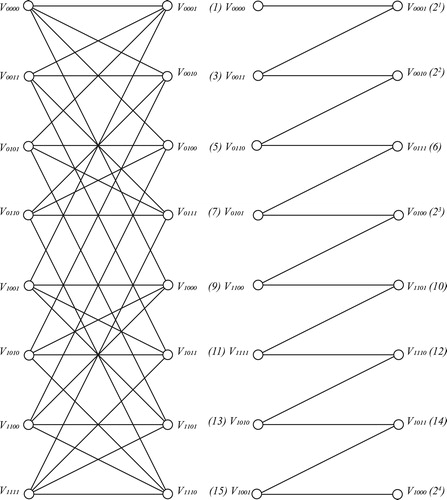
3.7 Theorem

Let $Q_n$ be an $n$-regular hypercube with the vertices partitioned into two disjoint subsets $V_1$ and $V_2$, containing $2^{n-1}$ vertices each. We introduce the Hamiltonian ordering for the vertices of $Q_n$ so that the vertices are numbered as 1, 2, 3, $2^2$, …, $2^n$. Let the first vertex be $v_{00\dots 0}$ in $V_1$ and adjacent vertices $v_{0\dots 01},v_{0\dots 010},v_{0\dots 100}$, …$v_{10\dots 0}$ in $V_2$ which are numbered as 2, $2^2$, $2^3$, …, $2^n$. The vertex labels corresponding to the generalized spline $p_{Q_n}$ defined for $Q_n$ are as follows:

1.	The vertex $v_{00\dots 0}$ is labeled with the element 0 $\in$ $R$, i.e, $p_{v_{0\dots 0}}$ $=$ 0.
2.	The vertex $v_{0\dots 01}$ which is adjacent to $v_{0\dots 0}$ is labeled as $p_{v_{0\dots 01}}$ and is equal to the product of the $n$ elements belonging to the edge ideals associated with the $n$ edges adjacent to $v_{00...01}$.

Then, $$p_{v_{00...01}}={\alpha }_{0\dots 01,0\dots 00}{\alpha }_{00\dots 01,0\dots 011}{\alpha }_{00\dots 01,0\dots 0101}\dots {\alpha }_{00\dots 01,10\dots 01}$$

Similarly the vertex $v_{00...10}$ is labeled as $p_{v_{0\dots 10}}$ associated with the $n$ edges adjacent to the vertex $v_{00...010}$. Then,

$p_{v_{00...010}}={\alpha }_{0\dots 10,0\dots 00}{\alpha }_{00\dots 10,0\dots 011}{\alpha }_{00\dots 10,0\dots 0110}$…${\alpha }_{00\dots 10,10\dots 010}$ and so on.

These are the only vertices with non-zero vertex labels where each vertex label is a product of $n$ elements belonging to $n$ edge ideals and the remaining vertices are labeled as zero.

It can be easily verified that $p_{Q_n}$ is a generalized spline on the hypercube $Q_n$ as the edge conditions are satisfied for the adjacent vertices and also, $p_{Q_n}$ is nontrivial since $R$ is an integral domain.

4 Conclusions

We conclude our work by developing an algorithm to construct the generalized spline rings for the special graphs such as the complete graphs, complete bipartite graphs and hypercubes. These graphs find important applications in network and approximation theory and the present work adds to the existing knowledge and understanding in these and related areas. Also, it opens a vast field for research as we can think of studying the generalized splines over these and other graphs by changing the base rings to other rings such as the polynomial rings and ring of Laurent polynomials. As these rings are PIDs, we can also try to find suitable bases for the generalized splines for these graphs.

5 List of abbreviations

The following are the list of abbreviations used in this paper:

1. CAGD: Computer-Aided Geometric Design

2. PID: Principal Ideal Domain

References

- BilleraL.J.RoseL.L., A dimension series for multivariate splines Discrete Comput. Geom. 6 2 1991 107–128. 10.1007/BF02574678
- DummitD.Foote.R.Abstract AlgebraInternational Series of Monographs on Physics2003Wiley
- HaasR., Module and vector space bases for spline spaces J. Approx. Theory 65 1 1991 73–89
- RoseL.L., Graphs, syzygies, and multivariate splines Discrete Comput. Geom. 32 4 2004 623–637. 10.1007/s00454-004-1141-3
- DiPasqualeM.R., Shellability and freeness of continuous splines J. Pure Appl. Algebra 216 11 2012 2519–2523. 10.1016/j.jpaa.2012.03.010
- DalbecJ.P.SchenckH., On a conjecture of rose J. Pure Appl. Algebra 165 2 2001 151–154. 10.1016/S0022-4049(00)00175-4URLhttp://www.sciencedirect.com/science/article/pii/S0022404900001754
- BilleraL.J.RoseL.L., Modules of piecewise polynomials and their freeness Math. Z. 209 1 1992 485–497. 10.1007/BF02570848
- YuzvinskyS., Modules of splines on polyhedral complexes Math. Z. 210 1 1992 245–254. 10.1007/BF02571795
- J. Tymoczko, Splines in geometry and topology, ArXiv e-prints (11 2015).
- N. Bowden, J. Tymoczko, Splines mod m, ArXiv e-prints (2015).
- S. Gilbert, S. Polster, J. Tymoczko, Generalized splines on arbitrary graphs, ArXiv e-prints (2013).
- M. Handschy, J. Melnick, S. Reinders, Integer Generalized Splines on Cycles, ArXiv e-prints (sep 2014).arXiv:1409.1481.
- S. F. Florkowski III, Spectral graph theory of the hypercube, Tech. rep. NAVAL POSTGRADUATE SCHOOL MONTEREY CA (2008).
- DybizbaskiJ.SzepietowskiA., Hamiltonian paths in hypercubes with local traps Inform. Sci. 3752017 258–270. 10.1016/j.ins.2016.10.011URLhttp://www.sciencedirect.com/science/article/pii/S0020025516311756
- E. Gjoni, Basis criteria for n-cycle integer splines, Bard College Senior Projects Spring (2015).
- NikolopoulosS.D., Optimal gray-code labeling and recognition algorithms for hypercubes Inform. Sci. 137 1 2001 189–210. 10.1016/S0020-0255(01)00120-7URLhttp://www.sciencedirect.com/science/article/pii/S0020025501001207
- WestDouglas B., Introduction to Graph Theory2000Prentice Hall