Mathematical modeling of gas phase and biofilm phase biofilter performance

Abstract

In this paper, mathematical models of biofilteration of mixtures of hydrophilic (methanol) and hydrophobic (α-pinene) volatile organic compounds (VOC's) biofilters were discussed. The model proposed here is based on the mass transfer in air–biofilm interface and chemical oxidation in the air stream phase. An approximate analytical expression of concentration profiles of methanol and α-pinene in air stream and biofilm phase have been derived using the Adomian decomposition method (ADM) for all possible values of parameters. Furthermore, in this work, the numerical simulation of the problem is also reported using the Matlab program to investigate the dynamics of the system. Graphical results are presented and discussed quantitatively to illustrate the solution. Good agreement between the analytical and numerical data is noted.

Keywords:

• Methanol
• Biofilters
• VOCs
• Mathematical modeling
• Non-linear differential equations
• Adomian decomposition method

1 Introduction

Different cleaning technologies of gaseous effluents have been developed. Among these technologies, biological methods are increasingly applied for the treatment of air polluted by a wide variety of pollutants. Biofilteration is certainly the most commonly used biological gas treatment technology. Biofilteration involves naturally occurring microorganisms immobilized in the form of biofilm on a porous medium such as peat, soil, compost, synthetic substances or their combination.

The medium provides to the microorganisms a hospitable environment in terms of oxygen, temperature, moisture, nutrients and pH. As the polluted airstream passes through the filter-bed, pollutants are transferred from the vapor phase to the biofilm developing on the packing particles [1,2].

Recently Li et al. [3] as well as other research groups [4–^{[5][6][7][8][9]}10] have investigated emissions of VOCs into the atmosphere. Currently, biological control processes have become an established technology for air pollution control. Biological control processes have many advantages over traditional methods such as lower operating fees and less secondary pollution, which is rather true for the removal of readily biodegradable VOCs at low concentrations, so these processes are investigated largely and widely. Bioreactors for VOC removal can be classified as biofilters, bio scrubbers, biotrickling filters, or rotating drum biofilters, and choice of reactors should be based on many factors including the characteristics of the target VOCs [11–^[12]15].

In order to control the emission of volatile organic compounds (VOC) like methanol, α-pinene, etc. from industries, biofilters are being used nowadays instead of chemical complex absorption method [16–^[17][18][19]20]. Biofilters offer two major advantages to an energy-starved country like India. A mathematical model is describing the dynamic physical and biological processes occurring in a packed trickle-bed air biofilters to analyze the relationship between biofilter performance and biomass accumulation in the reactor [4].

For the treatment of mixed VOCs [21–^[22]23], the presence of methanol and α-pinene in the air stream significantly influenced the removal of pollutants. The removal capacity for methanol and α-pinene per unit volume of the bed decreased linearly with increasing loading rates of methanol and α-pinene. The presence of this easily biodegradable compound suppressed the growth of the methanol and α-pinene degrading microbial community, thereby decreasing methanol and α-pinene removal capacity of the biofilters. Some researchers have studied the biofitration of pure methanol [24–^[25]26] and pure α-pinene [27,28].

Recently, few researchers have studied the biofitration of mixtures of pure methanol and pure α-pinene. Also a few researchers have tried to examine the treatment of mixtures of hydrophobic and hydrophilic VOCs and to understand the interactions between these compounds despite the fact that this situation exists in larger amount of air emissions. Mohseni and Allen [16] developed a mathematical model for methanol and α-pinene removal in VOC's biofilteration. Lim et al. [29] developed the steady state solution of biofilter model only for the limiting cases (first order and zero order kinetics). Also Lim et al. [30,31] obtained the non-steady solution of biofilter model using numerical methods. Recently some authors [32,33] solved the non-linear problems using fractional reduced differential transform method (FRDTM). To the best of our knowledge, to date, a rigorous analytical expression of concentrations of substrate in the biofilm phase and air phase has been reported. The purpose of this communication is to derive approximate analytical expressions for the concentrations in both the phases using the Adomian decomposition method [34–^[35]40].

2 Mathematical modeling of the boundary value problem

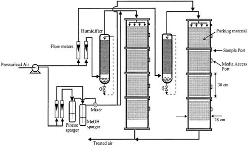
The mathematical model relating the biofiltration of blends of hydrophilic and hydrophobic VOCs is based on the biophysical model proposed by Mohseni and Allen [16]. It includes two main processes of diffusion of the compounds methanol and α-pinene through the biofilm and their degradation in the biofilm. Fig. 1 illustrates a schematic diagram of a single particle, in the biofilter, covered with a uniform layer of biofilm in which the simultaneous biodegradation of methanol and α-pinene takes place. The experimental setup for the biofilteration of this organic compound is given in Fig. 2.

Fig. 1 Biophysical model for the biofilm structure on the biofilters packing materials and the concentration profiles across the biofilm.

Fig. 2 Experimental setup for the bio filtration of methanol and α-pinene.

2.1 Mass balance in the biofilm phase

The removal of methanol and α-pinene in the biofilm at steady state is described by the following system of non-linear differential equations (Mohseni and Allen [16]):(1) $D_{em}\frac{d^2{S}_m}{d{x}^2}=\frac{X}{Y_m}\frac{{\mu }_{\max \left(m\right)}{S}_m}{K_m+S_m}$(1) (2) $D_{ep}\frac{d^2{S}_p}{d{x}^2}=\alpha \frac{X}{Y_p}\frac{{\mu }_{\max \left(p\right)}{S}_p}{K_p+S_p}$(2) where S_m and S_prepresent the concentration of methanol and α-pinene respectively.${\mu }_{\max }\text{},K,Y,D_e\text{and}x$ are maximum specific growth rate, half saturation constant, yield coefficient, effective diffusion coefficient and the distance respectively. Subscripts m and p represent methanol and α-pinene respectively. The dry cell density in the biofilm X represents the overall population of microorganisms that consist of methanol and α-pinene degraders. The coefficient for the effect of methanol on α-pinene biodegradation is defined as follows:(3) $\alpha =1/{\left(1+\left(C_m/K_i\right)\right)}^2$(3) where K_i and C_m are the inhibition constant and the concentration of methanol in the air phase respectively. The boundary conditions are(4) $S_m=\frac{C_m}{m_m}=S_{im}\text{and}{S}_P=\frac{C_P}{m_P}=S_{iP}\text{at}x=0$(4) (5) $\frac{d{S}_m}{dx}=\frac{d{S}_P}{dx}=0\text{at}x=\delta$(5)

2.2 Mass balance in gas phase

The concentrations of methanol and α-pinene in the air, along the biofilter column, are described by(6) $U_g\frac{d{C}_m}{dh}=A_s{D}_{em}{\left[\frac{d{S}_m}{dx}\right]}_{x=0}$(6) (7) $U_g\frac{d{C}_p}{dh}=A_s{D}_{ep}{\left[\frac{d{S}_{mp}}{dx}\right]}_{x=0}$(7) where C_m and C_p represent the concentration of methanol and α- pinene in the air phase. $U_g\text{},A_s\text{},D_{em}\text{},D_{ep}\text{and}h$ are the superficial gas velocity, biofilm surface area, effective diffusivity of methanol, effective diffusivity of α-pinene and position along the height of the biofilters respectively. The corresponding initial conditions are(8) $C_m=C_{mi}\text{and}{C}_p=C_{pi}\text{at}h=0$(8) where the subscript i represents the concentration of the VOCs at the biofilters inlet.

2.3 Dimensionless mass balance equation in the biofilm phase

The non-linear differential Eqs. (1)(1) $D_{em}\frac{d^2{S}_m}{d{x}^2}=\frac{X}{Y_m}\frac{{\mu }_{\max \left(m\right)}{S}_m}{K_m+S_m}$(1) and (2)(2) $D_{ep}\frac{d^2{S}_p}{d{x}^2}=\alpha \frac{X}{Y_p}\frac{{\mu }_{\max \left(p\right)}{S}_p}{K_p+S_p}$(2) are made dimensionless by defining the following dimensionless parameters:(9) $\beta =\frac{S_{im}}{K_m},{\phi }_1=\frac{X{\mu }_{\max \left(m\right)}}{Y_m}\frac{{\delta }^2}{D_{em}{K}_m},S_m\text{}*=\frac{S_m}{S_{im}}$(9) (10) ${\beta }_1=\frac{S_{ip}}{K_p},{\phi }_1=\frac{X{\mu }_{\max \left(p\right)}}{Y_p}\frac{{\delta }^2}{D_{ep}{K}_p},S_p\text{}*=\frac{S_p}{S_{ip}}$(10)

Using the above dimensionless variables, Eqs. (1)(1) $D_{em}\frac{d^2{S}_m}{d{x}^2}=\frac{X}{Y_m}\frac{{\mu }_{\max \left(m\right)}{S}_m}{K_m+S_m}$(1) and (2)(2) $D_{ep}\frac{d^2{S}_p}{d{x}^2}=\alpha \frac{X}{Y_p}\frac{{\mu }_{\max \left(p\right)}{S}_p}{K_p+S_p}$(2) reduce to the following dimensionless form:(11) $\frac{d^2{S}_m^{*}}{dX{*}^2}=\phi \left(\frac{S_m^{*}}{1+\beta S_m^{*}}\right)$(11) (12) $\frac{d^2{S}_p^{*}}{dX{*}^2}=\alpha {\phi }_1\left(\frac{S_p^{*}}{1+{\beta }_1{S}_p^{*}}\right)$(12)

The corresponding boundary conditions for the above Eqs. (11)(11) $\frac{d^2{S}_m^{*}}{dX{*}^2}=\phi \left(\frac{S_m^{*}}{1+\beta S_m^{*}}\right)$(11) and (12)(12) $\frac{d^2{S}_p^{*}}{dX{*}^2}=\alpha {\phi }_1\left(\frac{S_p^{*}}{1+{\beta }_1{S}_p^{*}}\right)$(12) can be expressed as(13) $S_m\text{}*=1,S_p\text{}*=1\text{at}X*=0$(13) (14) $\frac{d{S}_m\text{}*}{dX*}=\frac{d{S}_p\text{}*}{dX*}=0\text{at}X*=1$(14)

2.4 Dimensionless mass balance in the gas phase

The differential Eqs. (6)(6) $U_g\frac{d{C}_m}{dh}=A_s{D}_{em}{\left[\frac{d{S}_m}{dx}\right]}_{x=0}$(6) and (7)(7) $U_g\frac{d{C}_p}{dh}=A_s{D}_{ep}{\left[\frac{d{S}_{mp}}{dx}\right]}_{x=0}$(7) are made dimensionless by defining the following parameters:(15) $A=\frac{H{A}_s{D}_{em}{S}_{im}}{U_g\delta C_{mi}},A_1=\frac{H{A}_s{D}_{ep}{S}_{ip}}{U_g\delta C_{pi}},h*=\frac{h}{H},C_m^{*}=\frac{C_m}{C_{mi}},C_p^{*}=\frac{C_p}{C_{pmi}}$(15)

Using Eq. (15)(15) $A=\frac{H{A}_s{D}_{em}{S}_{im}}{U_g\delta C_{mi}},A_1=\frac{H{A}_s{D}_{ep}{S}_{ip}}{U_g\delta C_{pi}},h*=\frac{h}{H},C_m^{*}=\frac{C_m}{C_{mi}},C_p^{*}=\frac{C_p}{C_{pmi}}$(15) , Eqs. (6)(6) $U_g\frac{d{C}_m}{dh}=A_s{D}_{em}{\left[\frac{d{S}_m}{dx}\right]}_{x=0}$(6) and (7)(7) $U_g\frac{d{C}_p}{dh}=A_s{D}_{ep}{\left[\frac{d{S}_{mp}}{dx}\right]}_{x=0}$(7) can be expressed in the dimensionless form as follows:(16) $\frac{d{C}_m^{*}}{dh*}=-A{\left(\frac{d{S}_m^{*}}{dX*}\right)}_{X*=0}$(16) (17) $\frac{d{C}_{mp}^{*}}{dh*}=-\alpha A_1{\left(\frac{d{S}_p^{*}}{dX*}\right)}_{X*=0}$(17)

The corresponding initial conditions for the above Eqs. (16)(16) $\frac{d{C}_m^{*}}{dh*}=-A{\left(\frac{d{S}_m^{*}}{dX*}\right)}_{X*=0}$(16) and (17)(17) $\frac{d{C}_{mp}^{*}}{dh*}=-\alpha A_1{\left(\frac{d{S}_p^{*}}{dX*}\right)}_{X*=0}$(17) can be expressed as(18) $C_m^{*}=\frac{C_m}{C_{mi}}\text{and}{C}_p^{*}=\frac{C_{mp}}{C_{pi}}\text{at}h*=0$(18)

3 Analytical expression for the concentration of methanol and α-pinene using the Adomian decomposition method (ADM)

In recent years, many authors have applied the ADM [35–^{[36][37][38][39]}40] to various problems and demonstrated the efficiency of the ADM for handling non-linear and solving various chemistry and engineering problems. Using ADM (refer to Appendix A), we can obtain the concentration of methanol and α-pinene in the biofilm phase (see Appendix B) as follows:(19) $\begin{array}{c}{S}_m^{*}\left(X*\right)=\frac{S_m\left(x\right)}{S_{im}}=1+\frac{X{\mu }_{\max \left(m\right)}{\delta }^2}{Y_m{D}_{em}\left(K_m+S_{im}\right)}\left(\frac{x^2}{2{\delta }^2}-\frac{x}{\delta }\right)\\ =1+\frac{\phi }{\left(1+\beta \right)}\left(\frac{X{*}^2}{2}-X*\right)\end{array}$(19) (20) $\begin{array}{c}{S}_p^{*}\left(X*\right)=\frac{S_p\left(x\right)}{S_{ip}}=1+\frac{X{\mu }_{\max \left(p\right)}\alpha {\delta }^2}{Y_p{D}_{ep}\left(K_p+S_{ip}\right)}\left(\frac{x^2}{2{\delta }^2}-\frac{x}{\delta }\right)\\ =1+\frac{\alpha {\phi }_1}{\left(1+{\beta }_1\right)}\left(\frac{X{*}^2}{2}-X*\right)\end{array}$(20)

Also solving Eqs. (6–7) and (16–17) using the analytical method, we can obtain the concentration of methanol and α-pinene in the air phase.(21) $C_m^{*}\left(h*\right)=\frac{C_m\left(h\right)}{C_{mi}}=1-\frac{A_{s}X{\mu }_{\max \left(m\right)\delta }}{Y_m{U}_g{K}_m\left(1+\left(S_{im}/K_m\right)\right)}h=1-\frac{A\phi }{\left(1+\beta \right)}h*$(21) (22) $C_p^{*}\left(h*\right)=\frac{C_p\left(h\right)}{C_{pi}}=1-\alpha \frac{A_{s}X{\mu }_{\max \left(p\right)\delta }}{Y_p{U}_g{K}_p\left(1+\left(S_{ip}/K_p\right)\right)}h=1-\frac{\alpha A_1{\phi }_1}{\left(1+{\beta }_1\right)}h*$(22)

4 Analytical expression for the concentrations of methanol and α-pinene for unsaturated (first order) kinetics

Now we consider the limiting case where the substrate concentrations of methanol and α-pinene in biofilm phase are relatively low. In this case $S_m\le K_m\text{and}{S}_p\le K_p$. Eqs. (1)(1) $D_{em}\frac{d^2{S}_m}{d{x}^2}=\frac{X}{Y_m}\frac{{\mu }_{\max \left(m\right)}{S}_m}{K_m+S_m}$(1) and (2)(2) $D_{ep}\frac{d^2{S}_p}{d{x}^2}=\alpha \frac{X}{Y_p}\frac{{\mu }_{\max \left(p\right)}{S}_p}{K_p+S_p}$(2) now reduce to the following form.(23) $D_{em}\frac{d^2{S}_m}{d{x}^2}=\frac{X{\mu }_{\max \left(m\right)}}{Y_m{K}_m}{S}_m$(23) (24) $D_{ep}\frac{d^2{S}_p}{d{x}^2}=\alpha \frac{X{\mu }_{\max \left(p\right)}}{Y_p{K}_p}{S}_p$(24)

The analytical expression for concentrations of methanol and α-pinene in the biofilm phase becomes(25) $S_m^{*}\left(X*\right)=\frac{S_m\left(x\right)}{S_{im}}=\frac{\cosh \left(\sqrt{\frac{X{\mu }_{\max \left(m\right)}}{Y_m{D}_{em}{K}_m}}\left(x-\delta \right)\right)}{\cosh \left(\sqrt{\frac{X{\mu }_{\max \left(m\right)}}{Y_m{D}_{em}{K}_m}}\delta \right)}=\frac{\cosh \sqrt{\phi }\left(X*-1\right)}{\cosh \sqrt{\phi }}$(25) (26) $S_p^{*}\left(X*\right)=\frac{S_p\left(x\right)}{S_{ip}}=\frac{\cosh \left(\sqrt{\frac{\alpha X{\mu }_{\max \left(p\right)}}{Y_p{D}_{ep}{K}_p}}\left(x-\delta \right)\right)}{\cosh \left(\sqrt{\frac{\alpha X{\mu }_{\max \left(p\right)}}{Y_p{D}_{ep}{K}_p}}\delta \right)}=\frac{\cosh \sqrt{\alpha {\phi }_1}\left(X*-1\right)}{\cosh \sqrt{\alpha {\phi }_1}}$(26)

Using Eqs. (6–7) and (25–26) we obtain the analytical expression of the concentrations of methanol and α-pinene in the air phase.(27) $\begin{array}{c}{C}_m^{*}\left(h*\right)=\frac{C_m\left(h\right)}{C_{mi}}=1-\frac{A_s{D}_{em}{S}_{im}}{U_g}\sqrt{\frac{X{\mu }_{\max \left(m\right)}}{Y_m{D}_{em}{K}_m}}\tanh \sqrt{\frac{X{\mu }_{\max \left(m\right)}}{Y_m{D}_{em}{K}_m}}\delta \\ =1-\left(A\sqrt{\phi }\tanh \sqrt{\phi }\right)h*\end{array}$(27) (28) $\begin{array}{c}{C}_p^{*}\left(h*\right)=\frac{Cp\left(h\right)}{C_{pi}}=1-\frac{A_s{D}_{ep}{S}_{ip}}{U_g}\sqrt{\frac{\alpha X{\mu }_{\max \left(p\right)}}{Y_p{D}_{ep}{K}_p}}\tanh \sqrt{\frac{\alpha X{\mu }_{\max \left(p\right)}}{Y_p{D}_{ep}{K}_p}}\delta \\ =1-\left(A_1\sqrt{\alpha {\phi }_1}\tanh \sqrt{\alpha {\phi }_1}\right)h*\end{array}$(28)

5 Analytical solutions for the concentrations of methanol and α-pinene for saturated (zero order) kinetics

Next we consider the limiting case where the substrate concentrations of methanol and α-pinene in biofilm phase is relatively high. In this case $S_m\ge K_m\text{and}{S}_p\ge K_p$ and Eqs. (1)(1) $D_{em}\frac{d^2{S}_m}{d{x}^2}=\frac{X}{Y_m}\frac{{\mu }_{\max \left(m\right)}{S}_m}{K_m+S_m}$(1) and (2)(2) $D_{ep}\frac{d^2{S}_p}{d{x}^2}=\alpha \frac{X}{Y_p}\frac{{\mu }_{\max \left(p\right)}{S}_p}{K_p+S_p}$(2) reduce to the following form.(29) $D_{em}\frac{d^2{S}_m}{d{x}^2}=\frac{X}{Y_m}{\mu }_{\max \left(m\right)}$(29) (30) $D_{ep}\frac{d^2{S}_p}{d{x}^2}=\alpha \frac{X}{Y_p}{\mu }_{\max \left(p\right)}$(30)

Then the analytical expressions for concentration of methanol and α-pinene in the biofilm phase are as follows:(31) $S_m^{*}\left(X*\right)=\frac{S_m\left(x\right)}{S_{im}}=1-\frac{2X{\mu }_{\max \left(m\right)}}{Y_m{D}_{em}{S}_{im}}x+\frac{X{\mu }_{\max \left(m\right)}}{Y_m{D}_{em}{S}_{im}}{x}^2=1+\frac{\alpha \phi }{\beta }\left(X{*}^2-2X*\right)$(31) (32) $S_p^{*}\left(X*\right)=\frac{S_p\left(x\right)}{S_{ip}}=1-\frac{2X{\mu }_{\max \left(p\right)}}{Y_p{D}_{ep}{S}_{ip}}x+\frac{X{\mu }_{\max \left(p\right)}}{Y_p{D}_{ep}{S}_{ip}}{x}^2=1+\frac{\alpha {\phi }_1}{{\beta }_1}\left(X{*}^2-2X*\right)$(32)

Using Eqs. (6–7) and (31–32), we obtain the analytical expression of the concentrations of methanol and α-pinene in the air phase.(33) $C_m^{*}\left(h*\right)=\frac{C_m\left(h\right)}{C_{mi}}=1-\frac{2X{\mu }_{\max \left(m\right)}{A}_s\delta h}{Y_m{U}_g}=1-\frac{2A\phi }{\beta }h*$(33) (34) $C_p^{*}\left(h*\right)=\frac{C_p\left(h\right)}{C_{pi}}=1-\frac{2\alpha X{\mu }_{\max \left(p\right)}{A}_s\delta h}{Y_p{U}_g}=1-\frac{2\alpha A_1{\phi }_1}{{\beta }_1}h*$(34)

6 Removal ratio of methanol and α-pinene

The percentage of the methanol removal ratio is(35) ${\text{methanol}}_R=\frac{C_{mi}^{*}-C_{mf}^{*}}{C_{mi}^{*}}\times 100$(35) where $C_{mi}^{*}\text{and}{C}_{mf}^{*}$ are the initial (before treatment) and the final (after treatment) concentrations of methanol in the air phase, respectively. The percentage of the α-pinene removal ratio is(36) $\alpha -{\text{pinene}}_R=\frac{C_{pi}^{*}-C_{pf}^{*}}{C_{pi}^{*}}\times 100$(36) where $C_{pi}^{*}$ and $C_{pf}^{*}$ are the initial (before treatment) and the final (after treatment) concentrations of α-pinene in the air phase respectively.

7 Numerical simulation

In order to investigate the accuracy of the ADM solution with a finite number of terms, the system of differential equations was solved numerically. To show the efficiency of the present method, our analytical results are compared with numerical results graphically. The analytical solution of the concentrations of methanol and α-pinene in air phase and biofilm phase are compared with simulation results in Figs. 3–^{Fig. 4Fig. 5}6. Upon comparison, it gives a satisfactory agreement for all values of the dimensionless parameters $S_m\text{}*\text{},S_p\text{}*\text{},C_m^{*}\text{and}{C}_p^{*}$. The detailed Matlab program for numerical simulation is provided in Appendices C and D.

Fig. 3 Dimensionless methanol concentration $S_m^{*}$ in the biofilm phase versus dimensionless distance X^* for the various values of the parameters β and φ. When (a) φ = 10, (b) φ = 100 for various values of the parameter β and (c) β = 10, (b) β = 100 for various values of the parameter φ. The key to the graph: solid line represents Eq. (19)(19) $\begin{array}{c}{S}_m^{*}\left(X*\right)=\frac{S_m\left(x\right)}{S_{im}}=1+\frac{X{\mu }_{\max \left(m\right)}{\delta }^2}{Y_m{D}_{em}\left(K_m+S_{im}\right)}\left(\frac{x^2}{2{\delta }^2}-\frac{x}{\delta }\right)\\ =1+\frac{\phi }{\left(1+\beta \right)}\left(\frac{X{*}^2}{2}-X*\right)\end{array}$(19) and the dotted line represents the numerical simulation.

Fig. 4 Dimensionless α-pinene concentration $S_p^{*}$ in the biofilm phase versus dimensionless distance X^* for the parameters $\alpha ,{\beta }_1\text{and}{\phi }_1$. The parameter α = 1 is fixed, when (a) φ₁ = 1, (b) φ₁ = 100 for various values of the parameter β₁ and (c) β₁ = 10, (b) β₁ = 100 for various values of the parameter φ₁.The key to the graph: solid line represents Eq. (20)(20) $\begin{array}{c}{S}_p^{*}\left(X*\right)=\frac{S_p\left(x\right)}{S_{ip}}=1+\frac{X{\mu }_{\max \left(p\right)}\alpha {\delta }^2}{Y_p{D}_{ep}\left(K_p+S_{ip}\right)}\left(\frac{x^2}{2{\delta }^2}-\frac{x}{\delta }\right)\\ =1+\frac{\alpha {\phi }_1}{\left(1+{\beta }_1\right)}\left(\frac{X{*}^2}{2}-X*\right)\end{array}$(20) and the dotted line represents the numerical simulation.

Fig. 5 Dimensionless methanol concentration $C_m^{*}$ in the air phase versus dimensionless height h^* for some fixed values of the parameters $A=70\text{and}{C}_{mi}=1$. When (a) β = 100 for various values of the parameter φ and (b) φ = 1 for various values of the parameter β. The key to the graph: solid line represents Eq. (21)(21) $C_m^{*}\left(h*\right)=\frac{C_m\left(h\right)}{C_{mi}}=1-\frac{A_{s}X{\mu }_{\max \left(m\right)\delta }}{Y_m{U}_g{K}_m\left(1+\left(S_{im}/K_m\right)\right)}h=1-\frac{A\phi }{\left(1+\beta \right)}h*$(21) and the dotted line represents the numerical simulation.

Fig. 6 Dimensionless α-pinene concentration $C_p^{*}$ in the air phase versus dimensionless height h^* for some fixed values of the parameters $\alpha =1,A_1=70,\text{and}{C}_{pi}=0.27$. When (a) β₁ = 10 for various values of the parameter φ₁ and (b) φ₁ = 0.1 for various values of the parameter β₁.The key to the graph: solid line represents Eq. (22)(22) $C_p^{*}\left(h*\right)=\frac{C_p\left(h\right)}{C_{pi}}=1-\alpha \frac{A_{s}X{\mu }_{\max \left(p\right)\delta }}{Y_p{U}_g{K}_p\left(1+\left(S_{ip}/K_p\right)\right)}h=1-\frac{\alpha A_1{\phi }_1}{\left(1+{\beta }_1\right)}h*$(22) and the dotted line represents the numerical simulation.

8 Results and discussion

Eqs. (19–22) represent the simple and new analytical expression of the concentrations of methanol and α-pinene in biofilm phase $S_m\text{}*\text{},S_p\text{}*$ and in the air phase $C_m\text{}*\text{},C_p\text{}*$respectively. The concentrations of methanol and α-pinene in the biofilm phase and the air phase depend upon the parameters φ and β. The variation in the dimensionless variable φ can be achieved by varying either the thickness or dry cell density of the biofilm. The parameter β depends upon the initial concentration and half saturation constant.

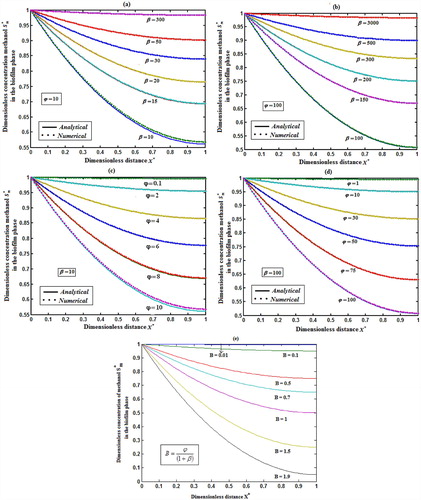
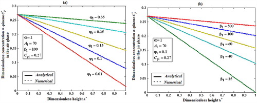
Fig. 3 represents the concentration of methanol $S_m\text{}*$ in the biofilm phase versus dimensionless distance X^* for different values of φ and β. From Fig. 3a, b, it is inferred that the concentration of methanol increases when the initial concentration of methanol β increases for the fixed values of φ. For large value of dimensionless parameter β, the concentration of methanol remains constant. In Fig. 3c, d, we present the concentration of methanol in the biofilm phase for various values of φ and for some fixed values of β. Maximum specific growth rate of methanol biodegradation φ decreases the concentration of methanol slowly and reaches the constant level. The minimum value of $S_m^{*}\left(X*\right)\text{and}{S}_p^{*}\left(X*\right)$ are $1-\left(\phi /2\left(1+\beta \right)\right)$ and $1-\left(\alpha {\phi }_1/2\left(1+{\beta }_1\right)\right)$ respectively.

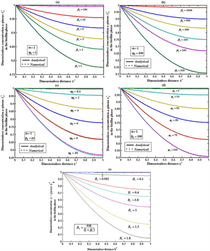
Fig. 4 exhibits the concentration of α-pinene $S_p\text{}*$ in the biofilm phase versus dimensionless distance X^* for different values of $\alpha ,{\phi }_1\text{and}{\beta }_1$. From Fig. 4a, b, it is inferred that the concentration of α-pinene increases when the initial concentration of α-pinene $\left({\beta }_1\right)$ increases for the fixed values of dry cell density φ₁. For large value of β₁, the concentration of α-pinene is uniform. In Fig. 4c, d, we show that the concentration of α-pinene in the biofilm phase for various values of cell density φ₁ and for some fixed values of dimensionless parameter β₁. From this figure, we conclude that the concentration of α-pinene $S_p\text{}*$ increases when thickness of the film decreases. The concentration of α-pinene is equal to one $\left(S_p\text{}*=1\right)$ when $\left(\phi /2\left(1+\beta \right)\right)<2$.

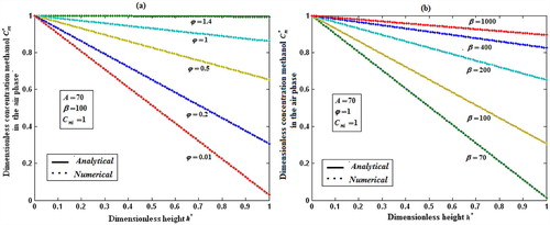
Fig. 5a, b shows the dimensionless concentration of methanol $C_m^{*}$ versus dimensionless height h^*. From Fig. 5a, it is described that the concentration of methanol slowly reaches the constant when the biofilm thickness or φ increases. In Fig. 5b, it is labeled that the concentration of methanol decreases when half saturation constant of methanol β decreases for the fixed value of other parameter.

Fig. 6a, b demonstrates the concentration of α-pinene $C_p^{*}$ in the air phase versus dimensionless height h^*. From Fig. 6a, it is inferred that the concentration of α-pinene slowly reaches a constant level when the diffusion coefficient φ₁ increases for the fixed value of other parameter. In Fig. 6b, it is labeled that the concentration of α-pinene attains the steady state values when the initial concentration of α-pinene $\left({\beta }_1\right)$ increases.

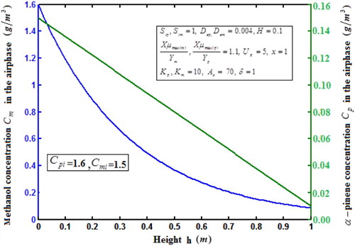
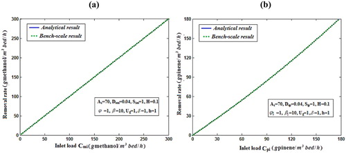
Fig. 7 shows the profile of dimension concentration of methanol and α-pinene in the air phase versus height h for some fixed value of the parameters. From these figures it is inferred that the concentration is linearly proportional to the height of the biofilter. And also the concentration of $C_m^{*}\text{and}{C}_p^{*}$ decrease when the height of the biofilter increases. Fig. 8a, b illustrates the removal ratio of methanol and α-pinene in the air phase. From this figure it is observed that the removal ratio is directly proportional to the inlet loading. Our analytical results are compared with the experimental result and excellent agreement is noted.

Fig. 7 Dimension methanol and α-pinene concentrations C_m and C_p in the air phase versus the height h using the values of the parameters$S_{im}\text{},S_{ip}=1,D_{em}\text{},D_{ep}=0.004,K_m\text{},K_p=10,$ respectively. The solid line represents Eqs. (21–22).

Fig. 8 (a) The methanol removal ratio ${\text{methanol}}_R$ versus inlet load C_mi for some fixed values of the parameters $A_s=70,D_{em}=0.04,S_{im}=1,H=0.1,\phi =1,\beta =10,U_g=1,\delta =1,,h=1$. The graph is plotted using Eq. (35)(35) ${\text{methanol}}_R=\frac{C_{mi}^{*}-C_{mf}^{*}}{C_{mi}^{*}}\times 100$(35) . (b) The α-pinene removal ratio $\alpha -{\text{pinene}}_{\mathrm{R}}$ versus inlet load ${\mathrm{C}}_{\text{pi}}$ for some fixed values of the parameters$A_s=70,D_{em}=0.04,S_{im}=1,H=0.1,{\phi }_1=1,{\beta }_1=10,U_g=1,\delta =1,,h=1$. The graph is plotted using Eqn. (36)(36) $\alpha -{\text{pinene}}_R=\frac{C_{pi}^{*}-C_{pf}^{*}}{C_{pi}^{*}}\times 100$(36) .

9 Conclusion

In this paper, the non-linear differential equations in biofiltration model have been solved analytically. Approximate analytical expressions pertaining to the concentrations of methanol and α-pinene in the biofilm phase for all the values of parameters are obtained using the Adomian decomposition method. This solution of the concentrations of methanol and α-pinene in the biofilm phase and air phase are compared with the numerical simulation results. This model is also validated using experimental results. These analytical results provide a good understanding of the system and the optimization of the parameters in biofiltration model.

Acknowledgements

This work was supported by the Department of Science and Technology (DST) (No. SB/S1/PC-50/2012). The authors are thankful to The Principal, The Madura College, Madurai and The Secretary, Madura College Board, Madurai for their encouragement.

Appendix A

Basic concepts of the Adomian decomposition method (ADM)

Consider the non-linear differential equation(A.1) $y^{″}+N\left(y\right)=g\left(x\right)$(A.1) with boundary conditions(A.2) $y\left(0\right)=A,y\left(b\right)=B$(A.2) where N(y) is a non-linear function, g(x) is the given function and A, B and b are given constants. We propose the new differential operator, as below(A.3) $L=\frac{d^2}{d{x}^2}$(A.3)

So, Eq. (A.1)(A.1) $y^{″}+N\left(y\right)=g\left(x\right)$(A.1) can be written as(A.4) $L\left(y\right)=g\left(x\right)-N\left(y\right)$(A.4)

The inverse operator $L^{-1}$ is therefore considered as a two-fold integral operator (Duan and Rach [37]), as below(A.5) $L^{-1}(.)={\displaystyle \underset{0}{\overset{x}{\int }}{\displaystyle \underset{b}{\overset{x}{\int }}(.)\mathit{dxdx}}}$(A.5)

Applying the inverse operator $L^{-1}$ on both sides of Eq. (A.4)(A.4) $L\left(y\right)=g\left(x\right)-N\left(y\right)$(A.4) yields(A.6) $y\left(x\right)=L^{-1}\left(g\left(x\right)\right)-L^{-1}\left(N\left(y\right)\right)+y^{\prime }\left(b\right)\left(x-0\right)+y\left(0\right),$(A.6)

Using the boundary conditions Eq. (A.2)(A.2) $y\left(0\right)=A,y\left(b\right)=B$(A.2) , Eq. (A.6)(A.6) $y\left(x\right)=L^{-1}\left(g\left(x\right)\right)-L^{-1}\left(N\left(y\right)\right)+y^{\prime }\left(b\right)\left(x-0\right)+y\left(0\right),$(A.6) becomes(A.7) $y\left(x\right)=L^{-1}\left(g\left(x\right)\right)-L^{-1}\left(N\left(y\right)\right)+Bx+A$(A.7)

The Adomian decomposition method introduces the solution y(x) and the non-linear function N(y) by infinite series(A.8) $y\left(x\right)={\displaystyle \sum _{n=0}^{\infty }{y}_n\left(x\right)}$(A.8) and(A.9) $N\left(y\right)={\displaystyle \sum _{n=0}^{\infty }{A}_n}$(A.9) where the components y_n(x) of the solution y(x) will be determined recurrently and the Adomian polynomials A_n of N(y) are evaluated using the formula(A.10) $A_n\left(x\right)=\frac{1}{n!}\frac{d^n}{d{\lambda }^n}N{\left({\displaystyle \sum _{n=0}^{\infty }{\lambda }^n{y}_n}\right)}_{\lambda =0}$(A.10) which gives(A.11) $\begin{array}{l}{A}_0=N\left(y_0\right),\\ A_1=N^{\prime }\left(y_0\right)y_1\text{},\\ A_2=N^{\prime }\left(y_0\right)y_2+\frac{1}{2}{N}^{″}\left(y_0\right)y_1^2\text{},\\ A_3=N^{\prime }\left(y_0\right)y_3+N^{″}\left(y_0\right)y_1{y}_2+\frac{1}{3!}{N^{\prime }}^{″}\left(y_0\right)y_1^3\text{},.\\ ⋮\end{array}$(A.11)

By substituting Eqs. (A.8)(A.8) $y\left(x\right)={\displaystyle \sum _{n=0}^{\infty }{y}_n\left(x\right)}$(A.8) and (A.9)(A.9) $N\left(y\right)={\displaystyle \sum _{n=0}^{\infty }{A}_n}$(A.9) in Eq. (A.7)(A.7) $y\left(x\right)=L^{-1}\left(g\left(x\right)\right)-L^{-1}\left(N\left(y\right)\right)+Bx+A$(A.7) gives(A.12) ${\displaystyle \sum _{n=0}^{\infty }{y}_n}=L^{-1}\left(g\left(x\right)\right)-L^{-1}\left({\displaystyle \sum _{n=0}^{\infty }{A}_n}\right)+Ax+B$(A.12)

Then equating the terms in the linear system of Eq. (A.11)(A.11) $\begin{array}{l}{A}_0=N\left(y_0\right),\\ A_1=N^{\prime }\left(y_0\right)y_1\text{},\\ A_2=N^{\prime }\left(y_0\right)y_2+\frac{1}{2}{N}^{″}\left(y_0\right)y_1^2\text{},\\ A_3=N^{\prime }\left(y_0\right)y_3+N^{″}\left(y_0\right)y_1{y}_2+\frac{1}{3!}{N^{\prime }}^{″}\left(y_0\right)y_1^3\text{},.\\ ⋮\end{array}$(A.11) gives the recurrent relation(A.13) $y_0=L^{-1}\left(g\left(x\right)\right)+Bx+A,y_{n+1}=-L^{-1}\left(A_n\right),n\ge 0$(A.13) which gives(A.14) $\begin{array}{l}{y}_0=L^{-1}\left(g\left(x\right)\right)+Ax+B,\\ y_1=-L^{-1}\left(A_0\right),\\ y_2=-L^{-1}\left(A_1\right),\\ y_3=-L^{-1}\left(A_2\right),.\\ ⋮\end{array}$(A.14)

From Eqs. (A.11)(A.11) $\begin{array}{l}{A}_0=N\left(y_0\right),\\ A_1=N^{\prime }\left(y_0\right)y_1\text{},\\ A_2=N^{\prime }\left(y_0\right)y_2+\frac{1}{2}{N}^{″}\left(y_0\right)y_1^2\text{},\\ A_3=N^{\prime }\left(y_0\right)y_3+N^{″}\left(y_0\right)y_1{y}_2+\frac{1}{3!}{N^{\prime }}^{″}\left(y_0\right)y_1^3\text{},.\\ ⋮\end{array}$(A.11) and (A.14)(A.14) $\begin{array}{l}{y}_0=L^{-1}\left(g\left(x\right)\right)+Ax+B,\\ y_1=-L^{-1}\left(A_0\right),\\ y_2=-L^{-1}\left(A_1\right),\\ y_3=-L^{-1}\left(A_2\right),.\\ ⋮\end{array}$(A.14) , we can determine the components y_n(x), and hence the series solution of y_n(x) in Eq. (A.7)(A.7) $y\left(x\right)=L^{-1}\left(g\left(x\right)\right)-L^{-1}\left(N\left(y\right)\right)+Bx+A$(A.7) can be immediately obtained.

Appendix B

Analytical solution of Eqs. (11)(11) $\frac{d^2{S}_m^{*}}{dX{*}^2}=\phi \left(\frac{S_m^{*}}{1+\beta S_m^{*}}\right)$(11) and (12)(12) $\frac{d^2{S}_p^{*}}{dX{*}^2}=\alpha {\phi }_1\left(\frac{S_p^{*}}{1+{\beta }_1{S}_p^{*}}\right)$(12)

In this appendix, we have derived the solution of Eqs. (11)(11) $\frac{d^2{S}_m^{*}}{dX{*}^2}=\phi \left(\frac{S_m^{*}}{1+\beta S_m^{*}}\right)$(11) and (12)(12) $\frac{d^2{S}_p^{*}}{dX{*}^2}=\alpha {\phi }_1\left(\frac{S_p^{*}}{1+{\beta }_1{S}_p^{*}}\right)$(12) using the Adomian decomposition method. Eq. (11)(11) $\frac{d^2{S}_m^{*}}{dX{*}^2}=\phi \left(\frac{S_m^{*}}{1+\beta S_m^{*}}\right)$(11) can be written with the operator form(B.1) $L(S_m^{*})=\phi N(S_m^{*})$(B.1) (B.2) $\text{wherethe differential operator}L=\frac{d^2}{dX{*}^2}\text{and}N(S_m^{*})=\frac{S_m^{*}}{1+\beta S_m^{*}}$(B.2)

Applying the inverse operator $L^{-1}(.)={\displaystyle \underset{0}{\overset{x*}{\int }}{\displaystyle \underset{1}{\overset{x*}{\int }}(.)dX*dX*}}$ on both sides of Eq. (B.1)(B.1) $L(S_m^{*})=\phi N(S_m^{*})$(B.1) yields(B.3) $S_m^{*}\left(X*\right)=AX*+B+\phi L^{-1}\left[\frac{S_m^{*}}{1+\beta S_m^{*}}\right]$(B.3) Where $A=S_m^{*}\prime \left(1\right)$ and $B=S_m^{*}\left(0\right)$. We let,(B.4) $S_m^{*}\left(X*\right)={\displaystyle \sum _{n=0}^{\infty }{S}_{m_n}^{*}\left(X*\right)}$(B.4) (B.5) $N[S_m^{*}\left(X*\right)]=\frac{S_m^{*}}{1+\beta S_m^{*}}={\displaystyle \sum _{n=0}^{\infty }{A}_n}$(B.5)

In view of Eqs. (B.4)(B.4) $S_m^{*}\left(X*\right)={\displaystyle \sum _{n=0}^{\infty }{S}_{m_n}^{*}\left(X*\right)}$(B.4) and (B.5)(B.5) $N[S_m^{*}\left(X*\right)]=\frac{S_m^{*}}{1+\beta S_m^{*}}={\displaystyle \sum _{n=0}^{\infty }{A}_n}$(B.5) , Eq. (B.3)(B.3) $S_m^{*}\left(X*\right)=AX*+B+\phi L^{-1}\left[\frac{S_m^{*}}{1+\beta S_m^{*}}\right]$(B.3) gives(B.6) ${\displaystyle \sum _{n=0}^{\infty }{S}_{m_n}^{*}\left(X*\right)}=AX*+B+\phi L^{-1}{\displaystyle \sum _{n=0}^{\infty }{A}_n}$(B.6)

We identify the zeroth component as(B.7) $S_{m_0}^{*}\left(x*\right)=AX*+B$(B.7) and the remaining components as the recurrence relation(B.8) $S_{m_{n+1}}^{*}\left(X*\right)=\phi L^{-1}{A}_n\text{},n\ge 0$(B.8) where A_n are the Adomian polynomials of $S_{m1}^{*}\text{},S_{m2}^{*}\cdots S_{mn}^{*}$. We can find the first few A_n as follows:(B.9) $A_0=N(S_{m0}^{*})=\frac{S_{m0}^{*}}{1+\beta S_{m0}^{*}}$(B.9) (B.10) $A_1={\frac{d}{d\lambda }[N(S_{m0}^{*}+\lambda S_{m1}^{*})]|}_{\lambda =0}=\frac{S_{m1}^{*}}{{\left(1+\beta \right)}^2}$(B.10)

The remaining polynomials can be generated easily, and so,(B.11) $S_{m0}^{*}\left(X*\right)=1$(B.11) (B.12) $S_{m1}^{*}\left(x*\right)=\frac{\phi }{\left(1+\beta \right)}\left(\frac{X{*}^2}{2}-X*\right)$(B.12)

Adding (B.11)(B.11) $S_{m0}^{*}\left(X*\right)=1$(B.11) and (B.12)(B.12) $S_{m1}^{*}\left(x*\right)=\frac{\phi }{\left(1+\beta \right)}\left(\frac{X{*}^2}{2}-X*\right)$(B.12) , we get Eq. (19)(19) $\begin{array}{c}{S}_m^{*}\left(X*\right)=\frac{S_m\left(x\right)}{S_{im}}=1+\frac{X{\mu }_{\max \left(m\right)}{\delta }^2}{Y_m{D}_{em}\left(K_m+S_{im}\right)}\left(\frac{x^2}{2{\delta }^2}-\frac{x}{\delta }\right)\\ =1+\frac{\phi }{\left(1+\beta \right)}\left(\frac{X{*}^2}{2}-X*\right)\end{array}$(19) in the text. Similarly, we can apply the above method to find the solution of Eq. (12)(12) $\frac{d^2{S}_p^{*}}{dX{*}^2}=\alpha {\phi }_1\left(\frac{S_p^{*}}{1+{\beta }_1{S}_p^{*}}\right)$(12) . Higher order iteration will be considered to improve the accuracy of the results.

Appendix C

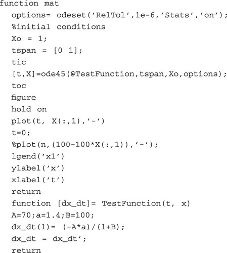
Matlab program for the numerical solution of Eqs. (11)(11) $\frac{d^2{S}_m^{*}}{dX{*}^2}=\phi \left(\frac{S_m^{*}}{1+\beta S_m^{*}}\right)$(11) and (12)(12) $\frac{d^2{S}_p^{*}}{dX{*}^2}=\alpha {\phi }_1\left(\frac{S_p^{*}}{1+{\beta }_1{S}_p^{*}}\right)$(12)

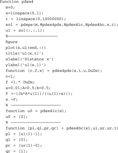
Appendix D

Matlab program for the numerical solution of Eqs. (16)(16) $\frac{d{C}_m^{*}}{dh*}=-A{\left(\frac{d{S}_m^{*}}{dX*}\right)}_{X*=0}$(16) and (17)(17) $\frac{d{C}_{mp}^{*}}{dh*}=-\alpha A_1{\left(\frac{d{S}_p^{*}}{dX*}\right)}_{X*=0}$(17)

Appendix E

Nomenclature

Table

Symbols	Definitions	Units
As	Biofilm surface area per unit volume of the biofilters	$m^2/m^3$
Cm	Concentration of methanol in the air stream	$g/m^3$
$C_{mi}$	Concentration of methanol in the inlet air stream	$g/m^3$
Cp	Concentration of α-pinene in the air stream	$g/m^3$
$C_{pi}$	Concentration of α-pinene in the inlet air stream	$g/m^3$
$D_{em}$	Effective diffusivity of methanol in the biofilm	$m^2/h$
$D_{ep}$	Effective diffusivity of α-pinene in the biofilm	$m^2/h$
h	Dimension along the height of the biofilters	m
H	Total height of the biofilters	m
Ki	Inhibition constant for α-pinene in the presence of methanol	$g/m^3$
Km	Half saturation constant of methanol in Monod kinetics obtained from differential biofilters experiments	$g/m^3$
Kp	Half saturation constant of α-pinene in Monod kinetics	$g/m^3$
mm	Air/biofilm partition coefficient for methanol, dimensionless	–
mp	Air/biofilm partition coefficient for α-pinene, dimensionless -
Sm	Concentration of methanol in the biofilm	$g/m^3$
Sp	Concentration of α-pinene in the biofilm	$g/m^3$
Ug	Superficial velocity of air through the biofilters	m/s
X	Dry cell density of the biofilm	$kg/m^3$
Y	Organic carbon content of the biofilm	$g/g$
Ym	Biomass yield coefficient for methanol	$kg/\mathit{cell}/kg$methanol
Yp	Biomass yield coefficient for α-pinene	kg/cell/kg α-pinene
$S_m=\frac{C_m}{m_m}=S_{im}$	Initial concentration of methanol in the biofilm	$g/m^3$
$S_p=\frac{C_p}{m_p}=S_{ip}$	Initial concentration of α-pinene in the biofilm	$g/m^3$
L	Linear operator
An	Adomian polynomial
Greek letters
α	Coefficient for the effect of methanol on α-pinene biodegradation, dimensionless	–
δ	Biofilm thickness	m
${\mu }_{\max \left(m\right)}$	Maximum specific growth rate for methanol biodegradation	$h^{-1}$
${\mu }_{\max \left(p\right)}$	Maximum specific growth rate for α-pinene biodegradation	h^−1
ρb	Density of the biofilm	kg/m^3
Dimensionless Parameters:
$\beta =\frac{S_{im}}{K_m}$	Dimensionless constant of methanol in Monod kinetics obtained from differential biofilters experiments	–
$\phi =\frac{X{\mu }_{\max \left(m\right)}}{Y_m}\frac{{\delta }^2}{D_{em}{K}_m}$	Dimensionless parameter	–
$X*=\frac{x}{\delta }$	Dimensionless coordinate in dry cell density of the biofilm	–
$S_m\text{}*=\frac{S_m}{S_{im}}$	Dimensionless concentration of methanol in the biofilm	–
${\beta }_1=\frac{S_{ip}}{K_p}$	Dimensionless constant of α-pinene in Monod kinetics obtained from bench-scale biofiltration results	–
${\phi }_1=\frac{\alpha X{\mu }_{\max \left(m\right)}}{Y_m}\frac{{\delta }^2}{D_{em}{K}_m}$	Dimensionless parameter	–
$S_p\text{}*=\frac{S_p}{S_{ip}}$	Dimensionless concentration of α-pinene in the biofilm	–
$A=\frac{H{A}_s{D}_{em}{S}_{im}}{U_g\delta C_{mi}}$	Dimensionless parameter	–
$A_1=\frac{H{A}_s{D}_{ep}{S}_{ip}}{U_g\delta C_{pi}}$	Dimensionless parameter	–
$C_m^{*}=\frac{C_m}{C_{mi}}$	Dimensionless concentration of methanol in the air stream	–
$C_p^{*}=\frac{C_p}{C_{pi}}$	Dimensionless concentration of α-pinene in the air stream	–
$C_{mi}^{*}$	Initial (before treatment) concentration of methanol	–
$C_{mf}^{*}$	Finial (before treatment) concentration of methanol	–
$C_{pi}^{*}$	Initial (before treatment) concentration of α-pinene	–
$C_{pf}^{*}$	Initial (before treatment) concentration of α-pinene	–
$h*=\frac{h}{H}$	Dimensionless along the height of the biofilters	–