
Abstract
Exact solutions of nonlinear evolution equations (NLEEs) play a vital role to reveal the internal mechanism of complex physical phenomena. In this article, we implemented the modified simple equation (MSE) method for finding the exact solutions of NLEEs via the (2+1)-dimensional cubic Klein–Gordon (cKG) equation and the (3+1)-dimensional Zakharov–Kuznetsov (ZK) equation and achieve exact solutions involving parameters. When the parameters are assigned special values, solitary wave solutions are originated from the exact solutions. It is established that the MSE method offers a further influential mathematical tool for constructing exact solutions of NLEEs in mathematical physics.
1 Introduction
Nonlinear phenomena exist in all areas of science and engineering, such as fluid mechanics, plasma physics, optical fibers, biology, solid state physics, chemical kinematics, chemical physics and so on. It is well known that many NLEEs are widely used to describe these complex physical phenomena. Therefore, research to look for exact solutions of NLEEs is extremely crucial. So, to find effective methods to discover analytic and numerical solutions of nonlinear equations have drawn an abundance of interest by a diverse group of researchers. Accordingly, they established many powerful and efficient methods and techniques to explore the exact traveling wave solutions of nonlinear physical phenomena, such as, the Hirota’s bilinear transformation method (Hirota, Citation1973; Hirota and Satsuma, Citation1981), the tanh-function method (Malfliet, Citation1992; Nassar et al., Citation2011), the (G′/G)-expansion method (Wang et al., Citation2008; Zayed, Citation2010; Zayed and Gepreel, Citation2009; Akbar et al., Citation2012a,Citationb,Citationc,Citationd; Akbar and Ali, Citation2011a; Shehata, Citation2010), the Exp-function method (He and Wu, Citation2006; Akbar and Ali, Citation2011b; Naher et al., Citation2011, Citation2012), the homogeneous balance method (Wang, Citation1995; Zayed et al., Citation2004), the F-expansion method (Zhou et al., Citation2003), the Adomian decomposition method (Adomian, Citation1994), the homotopy perturbation method (Mohiud-Din, Citation2007), the extended tanh-method (Abdou, Citation2007; Fan, Citation2000), the auxiliary equation method (Sirendaoreji, Citation2004), the Jacobi elliptic function method (Ali, Citation2011), Weierstrass elliptic function method (Liang et al., Citation2011), modified Exp-function method (He et al., Citation2012), the modified simple equation method (Jawad et al., Citation2010; Zayed, Citation2011a, Zayed and Ibrahim, Citation2012; Zayed and Arnous, Citation2012), the extended multiple Riccati equations expansion method (Gepreel and Shehata, Citation2012; Gepreel, Citation2011a; Zayed and Gepreel, Citation2011) and others (Gepreel, Citation2011b,Citationc).
Table
The objective of this article is to look for new study relating to the MSE method to examine exact solutions to the celebrated (2+1)-dimensional cKG equation and the (3+1)-dimensional ZK equations to establish the advantages and effectiveness of the method. The cKG equation is used to model many different nonlinear phenomena, including the propagation of dislocation in crystals and the behavior of elementary particles and the propagation of fluxions in Josephson junctions. The (3+1)-dimensional Zakharov–Kuznetsov equation describes weakly nonlinear wave process in dispersive and isotropic media e.g., waves in magnetized plasma or water waves in shear flows.
The article is organized as follows: In Section 2, the MSE method is discussed. In Section 3 we exert this method to the nonlinear evolution equations pointed out above, in Section 4 physical explanation, in Section 5 comparisons and in Section 6 conclusions are given.
2 The MSE method
Suppose the nonlinear evolution equation is in the form,(2.1) where F is a polynomial of u(x, y, z, t) and its partial derivatives wherein the highest order derivatives and nonlinear terms are involved. The main steps of the MSE method (Jawad et al., Citation2010; Zayed, Citation2011a; Zayed and Ibrahim, Citation2012; Zayed and Arnous, Citation2012) are as follows:
- Step 1:
The traveling wave transformation,
(2.2) allows us to reduce Eq. Equation(2.1)
- Step 2:
We suppose that Eq. Equation(2.3)
- Step 3:
We determine the positive integer n appearing in Eq. Equation(2.4)
- Step 4:
We substitute Eq. Equation(2.4)
3 Applications
3.1 The (2+1)-dimensional cubic Klein–Gordon (cKG) equation
In this sub-section, first we will exert the MSE method to find the exact solutions and solitary wave solutions of the celebrated (2+1)-dimensional cKG equation,(3.1) where α and β are non zero constants.
The traveling wave transformation(3.2) transforms the Eq. Equation(3.1)
(3.1) to the following ODE:
(3.3) Balancing the highest order derivative and nonlinear term of the highest order, yields n = 1.
Thus, the solution Eq. Equation(2.4)(2.4) takes the form,
(3.4) where C0 and C1 are constants such that C1 ≠ 0, and ϕ(ξ) is an unspecified function to be determined. It is simple to calculate that
(3.5)
(3.6)
(3.7) Substituting the values of u, u″, and u3 into Eq. Equation(3.3)
(3.3) and equating the coefficients of ϕ0,ϕ−1,ϕ−2,ϕ−3 to zero, yields
(3.8)
(3.9)
(3.10)
(3.11) Solving Eq. Equation(3.8)
(3.8) , we obtain
And solving Eq. Equation(3.11)
(3.11) , we obtain
Case-I: When C0 = 0, we obtain trivial solution, therefore the case is rejected.
Case-II: When
Integrating, Eq. Equation(3.12)(3.12) with respect to ξ, we obtain
(3.13) Using Eq. Equation(3.13)
(3.13) , from Eq. Equation(3.10)
(3.10) , we obtain
(3.14) Upon integration, we obtain
(3.15) where a1 and a2 are constants of integration. Therefore, the exact solution of the cKG Eq. Equation(3.1)
(3.1) is
(3.16) Substituting the values of C0, C1, and l and simplifying, we obtain
(3.17) where ξ = x + y − λt.
We can arbitrarily choose the parameters a1 and a2. Therefore, if we set , Eq. Equation(3.17)
(3.17) reduces to:
(3.18) Again if we set
, Eq. Equation(3.17)
(3.17) reduces to:
(3.19) Using hyperbolic function identities, from Eqs. (3.Equation18)
(3.18) and Equation(3
(3.19) .19), we obtain the following periodic solutions
(3.20) And
(3.21)
Remark 1
Solutions (3.16)–(3.21) have been verified by substituting them back into the original equation and found correct.
3.2 The (3+1)-dimensional Zakharov–Kuznetsov (ZK) equation
Now we will study the MSE method to find exact solutions and then the solitary wave solutions to the (3+1)-dimensional ZK equation(3.22) where
(3.23) The traveling wave transformation Equation(3.23)
(3.23) reduces to Eq. Equation(3.22)
(3.22) to the following ODE:
(3.24) Integrating Eq. Equation(3.24)
(3.24) with respect to ξ, we obtain
(3.25) Balancing the highest order derivative u′ and nonlinear term u2, we obtain 2n = n + 1, which gives n = 1.
Therefore, the solution Equation(2.4)(2.4) takes the form
(3.26) where C0 and C1 are constants such that C1 ≠ 0, and ϕ(ξ) is an unstipulated function to be determined. It is easy to make out that
(3.27)
(3.28) Substituting the values of u, u′ and u2 from (3.26), (3.27), and (3.28) into Eq. Equation(3.25)
(3.25) and then equating the coefficients of ϕ0, ϕ−1, and ϕ−2 to zero, we respectively obtain
(3.29)
(3.30)
(3.31) From Eq. Equation(3.29)
(3.29) , we obtain
And from Eq. Equation(3.31)
(3.31) , we obtain
Case-I: When C0 = 0 Eqs. Equation(3.30)
Integrating Equation(3.33)(3.33) with respect to ξ, we obtain
(3.34) where a2 is a constant of integration.
Therefore, the exact solution of the (3+1)-dimensional ZK equation Equation(3.22)(3.22) is
(3.35) Substituting the values of C0 and C1 into Eq. Equation(3.35)
(3.35) and simplifying, we obtain
(3.36) where ξ = x + y + z − λt.
We can randomly choose the parameters a1 and a2. Setting , Eq. Equation(3.36)
(3.36) reduces to:
(3.37) Again setting
Eq. Equation(3.36)
(3.36) reduces to:
(3.38)
Case-II: When
Remark 2
Solutions (3.35)–(3.39) have been checked by substituting them back into the original equation and found correct.
4 Physical explanations
In this section, physical explanations of the determined solutions are illustrated to show the effectiveness and convenience of the MSE method for seeking exact solitary wave solution and periodic traveling wave solution of nonlinear wave equations named (2+1)-dimensional cKG equation and the (3+1)-dimensional ZK equation.
4.1 Explanations
4.1.1 The (2+1)-dimensional cubic Klein–Gordon (cKG) equation
The wave speed λ and the nonzero constants α, and β play an important role in the physical structure of the solutions obtained in Eqs. (3.18)–(3.21). Now we will discuss the physical structure of Eqs. (3.Equation18)(3.18) and Equation(3
(3.19) .19). For different values of λ, α and β the following cases arise in Eqs. (3.Equation18)
(3.18) and Equation(3
(3.19) .19):
- (i)
In Eqs. (3.18)–(3.21), the wave speed
- (ii)
If
- (iii)
If
- (iv)
If
- (v)
If
- (vi)
If
- (vii)
If
- (viii)
If
- (ix)
If
4.1.2 The (3+1)-dimensional Zakharov–Kuznetsov (ZK) equation
The wave speed λ and the nonzero constant a play a significant role in the physical structure of the solutions obtained in Eqs. (3.37)–(3.39). For different values of λ and a the following cases arise in Eqs. (3.37)–(3.39):
- (i)
In Eqs. (3.37)–(3.39) λ ≠ 0 and a ≠ 0. For other values of λ and a Eq. Equation(3.37)
- (ii)
If λ < 0 and a < 0 or a > 0 then Eq. Equation(3.39)
- (iii)
If λ > 0 and a > 0 then Eq. Equation(3.39)
- (iv)
If λ > 0 and a < 0 then Eq. Equation(3.39)
- (v)
In Eq. Equation(3.39)
4.2 Graphical representation
Some of our obtained traveling wave solutions are represented in the following figures via symbolic computation software Maple with explanations:
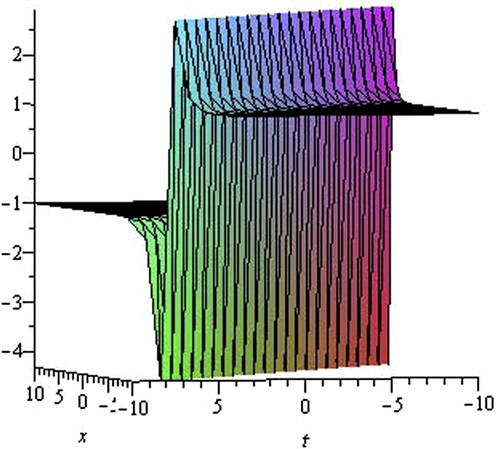
The solution Eq. Equation(3.18)(3.18) that comes infinity as in trigonometry, is Singular kink solution. shows the shape of the exact singular kink-type solution of the (2+1)-dimensional cKG Eq. Equation(3.1)
(3.1) (only shows the shape of Eq. Equation(3.18)
(3.18) with wave speed λ = −1, y = 2,α = 1, β = −1 and −10 ⩽ x,t ⩽ 10).
Figure 1 The shape of Eq. Equation(3.18)(3.18) with y = 2, λ = −1, α = 1, β = −1 and −10 ⩽ x,t ⩽ 10.
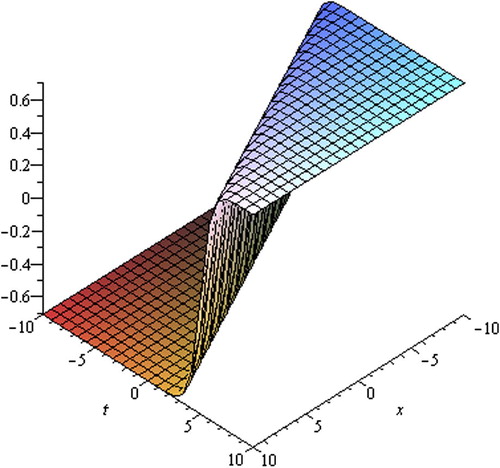
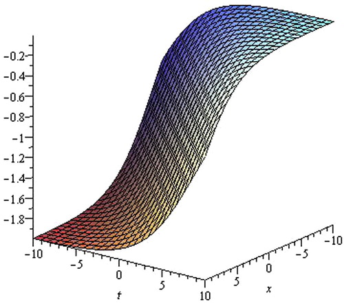
The solution Eq. Equation(3.19)(3.19) is called the kink solution. shows the shape of the exact kink-type solution of the (2+1)-dimensional cKG Eq. Equation(3.1)
(3.1) (only shows the shape of Eq. Equation(3.19)
(3.19) with wave speed λ = 2, y = 0,α = −1, β = 2 and −10 ⩽ x,t ⩽ 10)). The disturbance represented by u(x,y,t) is moving in the positive x-direction. If we take wave speed λ < 0, then the propagation will be in the negative x-direction.
Figure 2 The shape of Eq. Equation(3.19)(3.19) with y = 0,λ = 2,α = −1,β = 2 and −10 ⩽ x,t ⩽ 10.
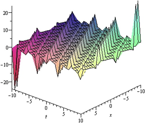
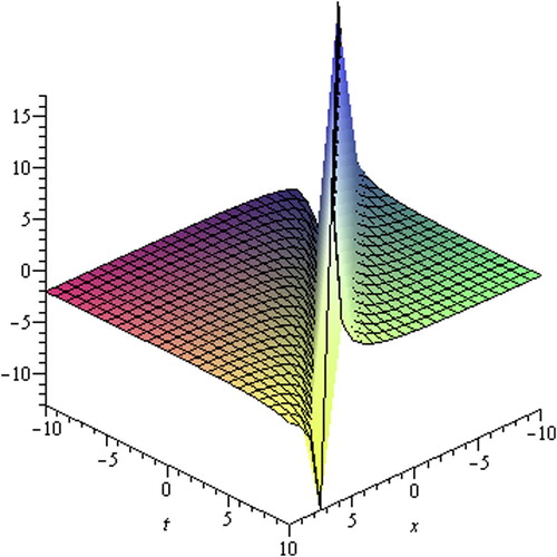
Eqs. (3.Equation20)(3.20) and Equation(3
(3.21) .21) are the exact periodic traveling wave solutions of the (2+1)-dimensional cKG Eq. Equation(3.1)
(3.1) , shapes are represented in and , respectively. shows the shape of Eq. Equation(3.20)
(3.20) with wave speed λ = 2, y = 2, α = 0.50,β = 1 in the interval −10 ⩽ x,t ⩽ 10 and shows the shape of Eq. Equation(3.21)
(3.21) with wave speed λ = 2, y = 0,α = 1,β = 2 in the interval − 10 ⩽ x,t ⩽ 10. The Eq. Equation(3.20)
(3.20) is singular periodic traveling wave solution and Eq. Equation(3.21)
(3.21) is periodic traveling wave solution.
Figure 3 The shape of Eq. Equation(3.20)(3.20) with λ = 2, y = 2, α = 0.5, β = 1 and −10 ⩽ x,t ⩽ 10.
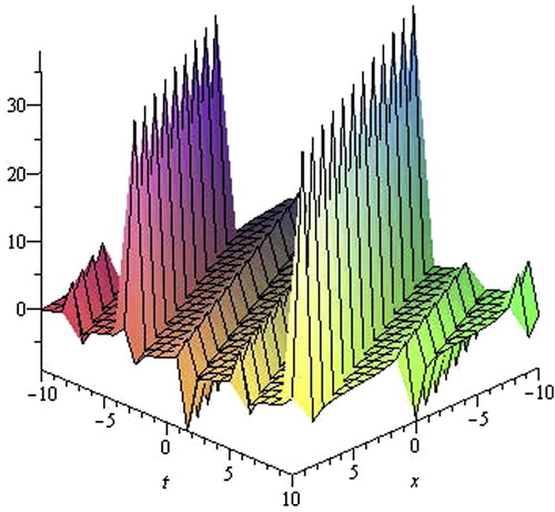
Figure 4 The shape of Eq. Equation(3.21)(3.21) with λ = 2, y = 0, α = 1, β = 2 and −10 ⩽ x,t ⩽ 10.
The solution Eqs. (3.Equation37)(3.37) and Equation(3
(3.39) .39) are the kink solutions. and show the shape of the exact kink-type solution of the (3+1)-dimensional ZK Eq. Equation(3.22)
(3.22) (only show the shape of Eq. Equation(3.37)
(3.37) with wave speed λ = 2,a = 1, y = z = 0 in the interval −10 ⩽ x, t ⩽ 10 and Eq. Equation(3.39)
(3.39) with wave speed λ = 1, a = −1, a1 = 1, a2 = −1, y = 1,z = 1 in the interval −10 ⩽ x, t ⩽ 10 respectively. The disturbance with y = z = 0 represented by u(x, y, z, t) is moving in the positive x-direction. If we take wave speed λ < 0 the propagation will be in the negative x-direction. These types of waves are traveling waves whose evolution from one asymptotical state at ξ → − ∞ to other asymptotical state at ξ → ∞.
Figure 5 The shape of Eq. Equation(3.37)(3.37) with λ = 2, a = 1, y = z = 0, −10 ⩽ x,t ⩽ 10.
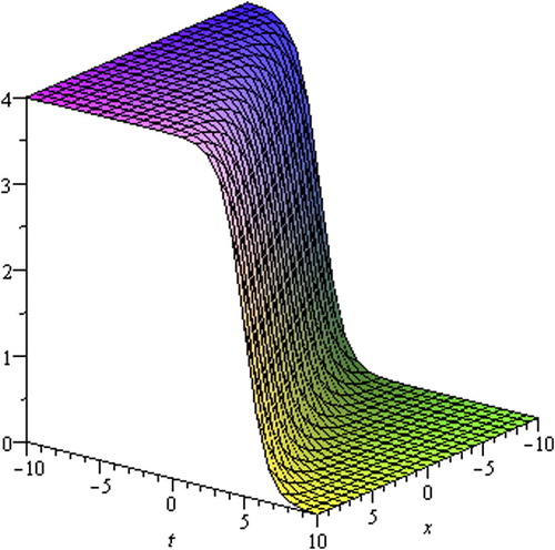
Figure 7 The shape of Eq. Equation(3.39)(3.39) with λ = 1, a = −1, a1 = 1, a2 = −1, y = z = 1, −10 ⩽ x,t ⩽ 10.
The solution Eq. Equation(3.38)(3.38) that comes infinity, is singular kink wave solution. shows the shape of the exact singular kink-type solution of the (3+1)-dimensional ZK Eq. Equation(3.22)
(3.22) (only shows the shape of Eq. Equation(3.38)
(3.38) with wave speed λ = 3, a = 1, y = 1, z = 2 and −10 ⩽ x, t ⩽ 10) (see ).
Figure 6 The shape of Eq. Equation(3.38)(3.38) with λ = 1, a = −1, y = 1, z = 2 and −10 ⩽ x,t ⩽ 10.
5 Comparison
Zayed (Citation2011b) studied solutions of the (2+1)-dimensional cKG equation using the (G′/G)-expansion method combined with the Riccati equation. The solutions of the (2+1)-dimensional cKG equation obtained by MSE method are different from those of the (G′/G)-expansion method combined with the Riccati equation (see Appendix). Comparing the MSE method with the (G′/G)-expansion method we might conclude that the exact solutions have investigated using the (G′/G)-expansion method with the help of the symbolic computation software, such as, Mathematica, Maple, to facilitate the complex algebraic computations. On the other hand via the MSE method the exact solutions to these equations have been achieved without using any symbolic computation software because the method is very simple and easy for computations. Moreover, in Exp-function method, tanh function method, Jacobi elliptic function method, (G′/G)-expansion method, etc., ϕ(ξ) is a pre-defined function or solution of a pre-defined differential equation. But, since in the MSE method ϕ (ξ) is not pre-defined or not solution of any pre-defined equation, some fresh solutions might be found. Consequently, much new and more general exact solutions of the (2+1)-dimensional cKG equation can be obtained by means of the MSE method with less effort.
6 Conclusions
In this article, we have found the traveling wave solutions of the (2+1)-dimensional cubic Klein–Gordon (cKG) equation and (3+1)-dimensional Zakharov–Kuznetsov (ZK) equation using the MSE method. These traveling wave solutions are expressed in terms of hyperbolic, and trigonometric functions involving arbitrary parameters. When these parameters are taken special values, the solitary waves are originated from the traveling waves. Compared to the methods used before, one can see that this method is direct, concise and effective. This method can also be used to many other nonlinear equations.
Acknowledgment
The authors would like to express their sincere thanks to the anonymous referee(s) for their detail comments and valuable suggestions.
Notes
Peer review under responsibility of University of Bahrain.
Related Research Data
References
- M.A.AbdouThe extended tanh-method and its applications for solving nonlinear physical modelsApp. Math. Comput.1902007988996
- G.AdomianSolving Frontier Problems of Physics: The Decomposition Method1994Kluwer AcademicBoston, MA
- M.A.AkbarN.H.M.AliThe alternative (G′/G)-expansion method and its applications to nonlinear partial differential equationsInt. J. Phys. Sci.635201179107920
- M.A.AkbarN.H.M.AliExp-function method for Duffing equation and new solutions of (2+1) dimensional dispersive long wave equationsProg. Appl. Math.1220113042
- M.A.AkbarN.H.M.AliE.M.E.ZayedAbundant exact traveling wave solutions of the generalized Bretherton equation via (G′/G)-expansion methodCommun. Theor. Phys.572012173178
- M.A.AkbarN.H.M.AliE.M.E.ZayedA generalized and improved (G′/G)-expansion method for nonlinear evolution equationsMath. Prob. Engr.201220122210.1155/2012/459879
- M.A.AkbarN.H.M.AliS.T.Mohyud-DinThe alternative (G′/G)-expansion method with generalized Riccati equation: application to fifth order (1+1)-dimensional Caudrey–Dodd–Gibbon equationInt. J. Phys. Sci.752012743752
- M.A.AkbarN.H.M.AliS.T.Mohyud-DinSome new exact traveling wave solutions to the (3+1)-dimensional Kadomtsev–Petviashvili equationWorld Appl. Sci. J.1611201215511558
- A.T.AliNew generalized Jacobi elliptic function rational expansion methodJ. Comput. Appl. Math.235201141174127
- E.G.FanExtended tanh-method and its applications to nonlinear equationsPhys. Lett. A2772000212218
- K.A.GepreelExact complexiton soliton solutions for nonlinear partial differential equationsInt. Math. Forum626201112611272
- K.A.GepreelA generalized (G′/G)-expansion method for finding traveling wave solutions of nonlinear evolution equationsJ. Partial Diff. Eq.2420115569
- K.A.GepreelExact solutions for nonlinear PDEs with the variable coefficients in mathematical physicsJ. Inf. Comput. Sci.62011003014
- K.A.GepreelA.R.ShehataExact complexiton soliton solutions for nonlinear partial differential equations in mathematical physicsSci. Res. Essays722012149157
- J.H.HeX.H.WuExp-function method for nonlinear wave equationsChaos Solitons Fract.302006700708
- Y.HeS.LiY.LongExact solutions of the Klein–Gordon equation by modified Exp-function methodInt. Math. Forum742012175182
- R.HirotaExact envelope soliton solutions of a nonlinear wave equationJ. Math. Phys.141973805810
- R.HirotaJ.SatsumaSoliton solutions of a coupled KDV equationPhys. Lett. A851981404408
- A.J.M.JawadM.D.PetkovicA.BiswasModified simple equation method for nonlinear evolution equationsAppl. Math. Comput.2172010869877
- M.S.LiangA method to construct Weierstrass elliptic function solution for nonlinear equationsInt. J. Modern Phys. B254201119311939
- M.MalflietSolitary wave solutions of nonlinear wave equationsAm. J. Phys.601992650654
- S.T.Mohiud-DinHomotopy perturbation method for solving fourth-order boundary value problemsMath. Prob. Engr.2007200711510.1155/2007/98602 Article ID 98602
- H.NaherA.F.AbdullahM.A.AkbarThe Exp-function method for new exact solutions of the nonlinear partial differential equationsInt. J. Phys. Sci.629201167066716
- H.NaherA.F.AbdullahM.A.AkbarNew traveling wave solutions of the higher dimensional nonlinear partial differential equation by the Exp-function methodJ. Appl. Math.20121410.1155/2012/575387 Article ID 575387
- H.A.NassarM.A.Abdel-RazekA.K.SeddeekExpanding the tanh-function method for solving nonlinear equationsAppl. Math.2201110961104
- A.R.ShehataThe traveling wave solutions of the perturbed nonlinear Schrodinger equation and the cubic–quintic Ginzburg Landau equation using the modified (G′/G)-expansion methodAppl. Math. Comput.2172010110
- SirendaorejiNew exact travelling wave solutions for the Kawahara and modified Kawahara equationsChaos Solitons Fract.192004147150
- M.WangSolitary wave solutions for variant Boussinesq equationsPhys. Lett. A1991995169172
- M.WangX.LiJ.ZhangThe (G′/G)-expansion method and travelling wave solutions of nonlinear evolution equations in mathematical physicsPhys. Lett. A3722008417423
- E.M.E.ZayedTraveling wave solutions for higher dimensional nonlinear evolution equations using the (G′/G)-expansion methodJ. Appl. Math. Informatics282010383395
- E.M.E.ZayedA note on the modified simple equation method applied to Sharma–Tasso–Olver equationAppl. Math. Comput.218201139623964
- E.M.E.ZayedThe (G′/G)-expansion method combined with the Riccati equation for finding exact solutions of nonlinear PDEsJ. Appl. Math. Informatics292011351367
- E.M.E.ZayedA.H.ArnousExact solutions of the nonlinear ZK–MEW and the Potential YTSF equations using the modified simple equation methodAIP Conf. Proc.1479201220442048
- E.M.E.ZayedK.A.GepreelThe (G′/G)-expansion method for finding the traveling wave solutions of nonlinear partial differential equations in mathematical physicsJ. Math. Phys.502009013502013514
- E.M.E.ZayedK.A.GepreelA series of complexiton soliton solutions for nonlinear Jaulent–Miodek PDEs using Riccati equations methodProc. R. Soc. Edinburgh A Math.141A201110011015
- E.M.E.ZayedS.A.H.IbrahimExact solutions of nonlinear evolution equations in mathematical physics using the modified simple equation methodChin. Phys. Lett.2962012060201
- E.M.E.ZayedH.A.ZedanK.A.GepreelOn the solitary wave solutions for nonlinear Hirota–Sasuma coupled KDV equationsChaos Solitons Fract.222004285303
- Y.B.ZhouM.L.WangY.M.WangPeriodic wave solutions to coupled KdV equations with variable coefficientsPhys. Lett. A30820033136
Appendix A
Zayed (Citation2011b) studied solutions of the (2+1)-dimensional cKG equation using the (G′/G)-expansion method and achieved the following calculations and exact solutions:(34) Consequently the following algebraic equations
(35) Which can be solved to get
(36) Substituting Equation(3.36)
(3.36) into Equation(3.4)
(3.4) yields
(37) where
(38) According to general solutions of the Riccati equations, he (Zayed, Citation2011b) got the following families of exact solutions:
Family 1. If
Family 2. If
Family 3. If A = 1,B = −1, then
Family 4. If A = B = 1, then
The general solutions of the Riccati equations G′(ξ) = A + BG2 are well known which are listed in the following table: