A new approach for a class of nonlinear boundary value problems with multiple solutions

Peer review under responsibility of University of Bahrain.

Abstract

In this paper, an approach based on the variational iteration method (VIM) is proposed with an auxiliary parameter to predict the multiplicity of the solutions of homogeneous nonlinear ordinary differential equations with boundary conditions. The proposed approach is capable to predict and calculate all branches of the solutions simultaneously. Four practical problems are chosen to show the efficiency and importance of the proposed method. The proposed approach successfully detects multiple solutions to Bratu’s problem, the model of mixed convection flows in a vertical channel, the nonlinear model of diffusion and reaction in porous catalysts and the nonlinear reactive transport model.

Keywords:

• Variational iteration method
• Multiple solutions
• Auxiliary parameter
• h-Curve
• Nonlinear boundary value problems

1 Introduction

Inokuti et al. (1978) proposed a general Lagrange multiplier method to solve nonlinear problems, which was intended to solve problems in quantum mechanics. Subsequently, He (1997) has modified the method to an iterative method and named it variational iteration method (VIM) and it has been presented by many authors to be a powerful mathematical tool for solving various types of nonlinear problems which represent plenty of modern science branches (He, 2012a, 2006; Yang and Baleanu, 2013; Wu, 2012). But this method cannot provide us with a simple way to adjust and control the convergence region and rate of giving approximate series, this reason was a strong motivation for authors to construct the variational iteration algorithms with an auxiliary parameter h which proves very effective to control the convergence region of an approximate solution as (He, 2012b; Hosseini et al., 2011; Turkyilmazoglu, 2011; Ghaneai et al., 2012; Hosseini et al., 2010) and others.

It is very important to predict and calculate all solutions of nonlinear differential equations with boundary conditions in engineering and physical sciences. In this regard, many authors constructed the algorithms that are based on the homotopy analysis method (HAM) for multiple solution of nonlinear boundary value problems as Li and Liao, 2005; Abbasbandy and Shivanian, 2011; Abbasbandy et al., 2009; Hassan and El-Tawil, 2011; Hassan and Semary, 2013" and others. However, in this work, the algorithm based on the variational iteration method (VIM) with an auxiliary parameter is presented in prediction and actual determination of multiple solutions of nonlinear boundary value problems. To show the efficiency and importance of the proposed method, four practical problems are solved. A problem arising in mixed convection flows in a vertical channel (Barletta, 1999; Barletta et al., 2005), Bratu’s problem (Wazwaz, 2012; Jalilian, 2010; Wazwaz, 2005), the nonlinear model of diffusion and reaction in porous catalysts (Sun et al., 2004; Abbasbandy, 2008; Magyari, 2008) and the nonlinear reactive transport model (Ellery and Simpson, 2011; Vosoughi et al., 2012), respectively and all of them admit multiple (dual) solutions which is why these models have been chosen to accomplish the article’s goal.

2 Analysis of the method

Consider the nonlinear differential equation(2.1) where L is a linear operator, N is a nonlinear operator and g(t) is an inhomogeneous term. According to the variational iteration method, one can construct an iteration formula for the Eq. (2.1)(2.1) as follows:(2.2) where λ(τ) is a general Lagrange multiplier, is considered as a restricted variation (He, 1998; He, 1999; Wazwaz, 2007; Wazwaz, 2009) which means . To solve (2.1)(2.1) by He’s VIM (He, 1997), we first determine the Lagrange multiplier λ(τ) that can be identified optimally via variational theory. Then, the successive approximations u_m+1(t), m ⩾ 0 of the solution u(t) can be readily obtained upon using the obtained Lagrange multiplier and by using any selective function u₀(t). The initial approximation u₀(t) may be selected by any function that just satisfies at least the initial and boundary conditions. With λ(τ) to be determined, several approximations u_m+1(t), m ⩾ 0, follow immediately. Consequently, the exact solution may be obtained by using the form(2.3) Ghaneai et al. (2012) constructed a variational iteration algorithm with an auxiliary parameter in the form(2.4) where h is an auxiliary parameter. The proposed approach to predict the multiplicity of the solutions of homogeneous nonlinear ordinary differential equations with boundary conditions based on the algorithm (2.4)(2.4) . Let the problem (2.1)(2.1) be the form(2.5) with the boundary condition(2.6)

Firstly by adding the new condition with unknown parameter α in the boundary conditions (2.6)(2.6) and splitting into(2.7) (2.8) where u(a) = b is called the forcing condition that comes from original conditions (2.6)(2.6) . By calculating variation with respect to u_m(τ) for variational iteration formula (2.2)(2.2) on the problem (2.5)(2.5) with the new initial conditions (2.7)(2.7) , the Lagrange multiplier λ(τ) can be identified as (He, 1998; He, 1999; Wazwaz, 2007; Wazwaz, 2009)(2.9) then the iteration formula (2.4)(2.4) becomes(2.10)

It should be emphasized that u_m+1(t,α,h) can be computed by symbolic software programs such as Mathematica or Maple, starting by an initial approximation u₀(t,α) which satisfies at least the initial conditions (2.7)(2.7) . We obtain the approximate solution u_m+1(t,α,h) for the problem (2.5)(2.5) and (2(2.7) .7), but there are still two unknown parameters in the approximate solution u_m+1 (t,α,h) the unknown parameter α and the auxiliary parameter h, should be determined. The forcing condition (2.8)(2.8) of the boundary value problem (2.5)(2.5) reads(2.11)

The Eq. (2.11)(2.11) has two unknown parameters α and h which control the approximation u_m+1(t,α,h) that converges to the exact solution. According to Eq. (2.11)(2.11) , α as function of h, by drawing the Eq. (2.11)(2.11) gives the so called h-curve. The number of such horizontal plateaus where α(h) becomes constant, gives the multiplicity of the solutions. Also the horizontal plateaus indicate the convergence because the unknown parameter α is a constant value then a horizontal line segment in h-curve which corresponds to the valid region of h.

3 Applications

3.1 Bratu’s problem

Consider Bratu’s problem in one-dimensional planar:(3.12) (3.13)

Bratu’s problem (3.12)(3.12) nonlinear two boundary value problem with strong nonlinear term e^u and parameter β, appears in a number of applications such as the fuel ignition model of the thermal combustion theory, the model of thermal reaction process, the Chandrasekhar model of the expansion of the Universe, questions in geometry and relativity about the Chandrasekhar model, chemical reaction theory, radiative heat transfer and nanotechnology (Wazwaz, 2012; Jalilian, 2010; Wazwaz, 2005). The analytical solution of (3.12)(3.12) and (3(3.13) .13) can be put in the following form:(3.14) where θ is a solution of . Bratu’s problem has no, one or two solutions when β > β_c, β = β_c and β < β_c respectively, where the critical value β_c satisfies the equation and also β_c = 3.513830719 (Wazwaz, 2012; Jalilian, 2010; Wazwaz, 2005). Differentiating (3.14)(3.14) with respect to x one time and setting x = 0 give(3.15)

In this study, we apply the present formula (2.10)(2.10) to detect dual solutions to Bratu’s problem for β = 3.

Direct application by the present formula (2.10)(2.10) to Bratu’s problem (3.12)(3.12) is very difficult, because they contain the strong nonlinear term e^u. To overcome this difficulty, differentiating (3.12)(3.12) with respect to x one time, for β = 3, Bratu’s problem (3.12)(3.12) and (3(3.13) .13) becomes(3.16) (3.17)

Firstly split the boundary conditions (3.17)(3.17) to(3.18) and the forcing condition(3.19)

Now, we apply the formula (2.10)(2.10) , in Eqs. (3.16)(3.16) and (3(3.18) .18), then(3.20) according to the conditions (3.18)(3.18) , we choose the initial approximation u₀(x,α) as:(3.21)

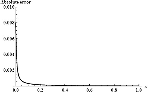
Using the Mathematica software, starting with u₀(x,α), the successive approximations u_m+1(x,α,h), m ⩾ 0 , can be as followsand so on, with the help of additional forcing condition (3.19)(3.19) , then(3.22) and(3.23) where u(x) is the exact solution (3.14)(3.14) . The exact values of u′(0) from Eq. (3.15)(3.15) are 2.319602 and 6.103 for β = 3. We got α as a function of h from (3.22)(3.22) that is plotted in Fig. 1. From Fig. 1, two values of α are clear (two line segments give constant values of α) the first and second intervals branch solution are [0.6,1.2] and [0.9,1.1], respectively, when h = 1.02, the first and second branch solutions of u′(0) = α are 2.319609 and 6.109, respectively. Comparing the values of u′(0) by the present approach and exact solution illustrates the accuracy of the present approach. Also, to show the accuracy of these dual approximate solutions, the absolute errors (3.23)(3.23) for first and second solutions are shown in Figs. 2 and 3, respectively. The Figs. 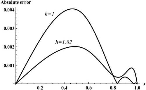2 and 3 show the present approach success to calculate the first and second solutions of Bratu’s problem (3.12)(3.12) for β = 3 and this means that the approach used is capable of detecting dual solution, also Fig. 3 shows effect of the auxiliary parameter h, by changing h from 1 to 1.02 the absolute error (3.23)(3.23) is improved.

Figure 1 Plot α as a function of h at m = 5 in (3.22)(3.22) of Bratu’s problem (3.16)(3.16) .

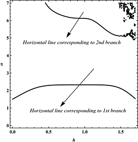
Figure 2 The absolute error (3.23)(3.23) for the first branch solution of Bratu’s problem (3.16)(3.16) when h = 1.

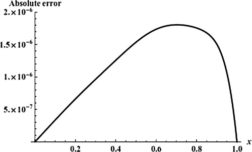
Figure 3 The absolute error (3.23)(3.23) for the second branch solution of Bratu’s problem (3.16)(3.16) when h = 1 and h = 1.02.

3.2 Mixed convection flows in a vertical channel

The aim of this section is to apply the present approach to detect the multiple solutions of a kind of model in mixed convection flows namely combined forced and free flow in the fully developed region of a vertical channel with isothermal walls kept at the same temperature (Barletta, 1999; Barletta et al., 2005). In this model, the fluid properties are assumed to be constant and the viscous dissipation effect is taken into account. The set of governing balance equations for the velocity field is reduced to(3.24) with the boundary conditions(3.25)

In the case E = 0, the Eqs. (3.24)(3.24) and (3(3.25) .25) are easily solved and admit the unique solution(3.26)

It has been shown in Abbasbandy and Shivanian, 2011; Barletta, 1999; Barletta et al., 2005" by semi-analytic and numerical methods that Eqs. (3.24)(3.24) and (3(3.25) .25) admit dual solutions for any given E in the interval ( −∞,0) ∪ (0,E_max) in which E_max ≅ 228.128. According to the initial conditions (2.7)(2.7) , the boundary condition (3.25)(3.25) , becomes(3.27) where γ and α are the unknown parameters and the additional forcing conditions(3.28) (3.29)

Now, we apply the formula (2.10)(2.10) , in equations (3.24)(3.24) and (3(3.27) .27), then(3.30) according to the conditions (3.27)(3.27) , we choose the initial approximation u₀(y,α,γ) as:(3.31)

Using the software of Wolfram’s Mathematica, starting with u₀ (y,α,γ), then, the successive approximations u_m+1 (y,α,γ,h), m ⩾ 0, as followsand so on, with the help of additional forcing conditions (3.28)(3.28) and (3(3.29) .29), then(3.32) (3.33)

Using the Eq. (3.33)(3.33) to delete the unknown parameter γ of the Eq. (3.32)(3.32) so that it contains only two unknown parameters α and h. Now, we consider a case study when E = 40. According to the Eq. (3.32)(3.32) , the unknown parameter α as a function of the auxiliary parameter h, has been plotted in the h-range [−0.5,2.5] in Fig. 4, for m = 6 and E = 40. Two α-plateaus (two line segments give constant values of α) can be identified in this figure, this means that there are two solutions. From Fig. 5(a) it is clear that the valid region of h for the first branch solution is [0.5,1.5], also from Fig. 5(b) it is clear that the valid region of h for the second branch solution is [0.8,1.2]. Figs. 6 and 7 plot α as a function of the auxiliary parameter h at m = 6 in Eq. (3.32)(3.32) for different values of E, these figures show the two solutions of α, this means that the approach used is capable of detecting dual solution.

Figure 4 Plot α as a function of h at m = 6 in (3.32)(3.32) for E = 40.

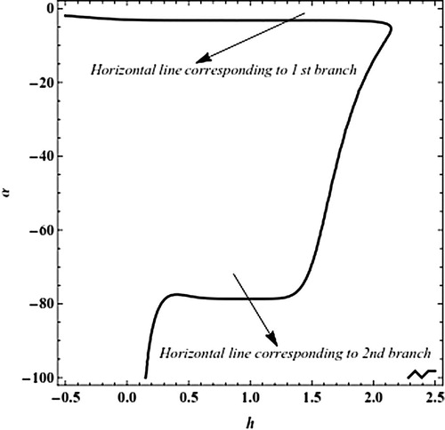
Figure 5 Plot α as a function of h at m = 6 in (3.32)(3.32) for E = 40, (a) the first branch solution and (b) the second branch solution.

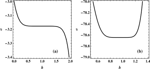
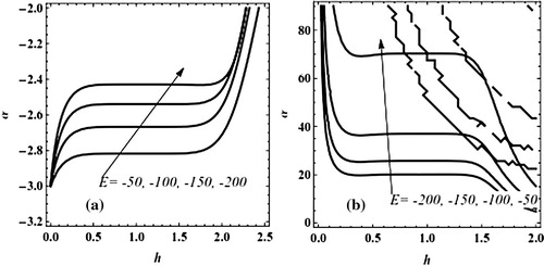
Figure 6 (a, b) Plot α as a function of h at m = 6 in (3.32)(3.32) for different values of positive E.

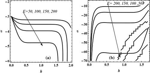
Figure 7 (a, b) Plot α as a function of h at m = 6 in (3.32)(3.32) for different values of negative E.

Table 1 Comparison between Predictor homotopy analysis method (PHAM) (Abbasbandy and Shivanian, 2011) and the present approach when m = 6 and h = 1 for the value of u″(0) = α for different values of E, from the table it is clear that results very close to the results of Abbasbandy and Shivanian, 2011, despite the number of iterations m = 6 are very few compared to the number of iterations m = 25 in (Abbasbandy and Shivanian, 2011).

Table 1 Comparison between the present approach and the predictor homotopy analysis method (PHAM) (Abbasbandy and Shivanian, 2011) of the value of u″(0) = α for different values of E.

E	First branch solution of α		Second branch solution of α
	Present algorithm	PHAM	Present algorithm	PHAM
−300	−2.244673	−2.24467	14.40219	14.4022
−200	−2.429229	−2.42923	20.138303	20.1383
−80	−2.725278	−2.72528	45.35358	45.3536
−20	−2.9230	−2.923	170.03931	170.039
20	−3.084108	−3.08411	−161.7259	−161.726
80	−3.394693	−3.39469	−36.92681	−36.9268
100	−3.525808	−3.52581	−28.49296	−28.493
200	−4.764798	−4.7648	−10.63485	−10.6349
228	−6.503207	−6.50321	−6.851835	−6.85183

3.3 The nonlinear model of diffusion and reaction in porous catalysts

The nonlinear model investigated recently (Sun et al., 2004; Abbasbandy, 2008; Magyari, 2008) describes the steady diffusion-reaction regime in a porous slab with parallel plane boundaries. In dimensionless variables the basic boundary value problem reads(3.34) (3.35)

As it has been shown in Magyari, 2008, the exact solution of the boundary value problem (3.34)(3.34) can be given in the implicit form(3.36) where α = u(0) and erf(…) denotes the error function. the Eq. (3.36)(3.36) can also be inverted to the explicit form(3.37) where Inverf (…) denotes the inverse of the error function (which can be handled by using for e.g. the software of Wolfram’s Mathematica) and from Eq. (3.38)(3.38) the possible values of α can be determined.(3.38)

We apply the present approach to detect dual solution of the problem (3.34)(3.34) and (3(3.35) .35) for a case study of φ = 0.7, firstly split the boundary conditions (3.35)(3.35) to(3.39) and the forcing condition(3.40)

Now, we apply the formula (2.10)(2.10) , in equations. (3.34)(3.34) and (3(3.39) .39), then(3.41) according to the conditions (3.39)(3.39) , we choose the initial approximation u₀(x,α) as:(3.42)

Using the software of Wolfram’s Mathematica, starting with u₀ (x,α), the successive approximations u_m+1(x,α,h), m > 0 , as followand so on. With the help of the additional forcing condition (3.40)(3.40) , becomes(3.43) and(3.44)

We consider a case study consist of φ = 0.7, exactly from Eq. (3.38)(3.38) the values of unknown parameter α are 0.65415 and 0.2078. Plot of α as function of h according to Eq. (3.43)(3.43) for m = 7 is shown in Fig. 8. The number of such horizontal plateaus where α(h) becomes constant, gives the multiplicity of the solutions. Two α-plateaus can be identified in this figure, namely α = 0.65417 in the range [1,1.5] of h and α = 0.2073 in the range [1.75,2] of h. Comparing the values of α by the present approach against to exact solution illustrates the accuracy of the present approach. Also, to show the accuracy of these dual approximate solutions, we have shown the absolute errors (3.44)(3.44) for first and second solutions in Figs. 9 and 10, respectively. The figures show the present approach success to calculate first and second branch solutions of the problem (3.34)(3.44) at φ = 0.7, this means that the approach used is capable of detecting dual solution.

Figure 8 Plot α as a function of h at m = 7 in (3.43)(3.43) for the problem (3.34)(3.34) at φ = 0.7.

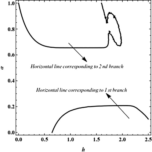
Figure 9 The absolute error (3.44)(3.44) of the first branch solution of the problem (3.34)(3.34) at h = 1.75.

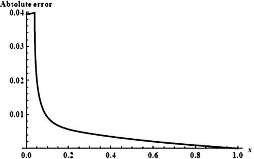
Figure 10 The absolute error (3.44)(3.44) of the second branch solution of the problem (3.34)(3.34) at h = 1.

3.4 The nonlinear reactive transport model

Consider dimensionless steady state reactive transport model which is governed by (Ellery and Simpson, 2011)(3.45) with boundary conditions(3.46)

The problem (3.45)(3.45) , recently introduced by Ellery and Simpson (2011) , is a kind of modification of the primer model so-called nonlinear reaction–diffusion model in porous catalysts which has been used to study porous catalyst pellets and more, it has been analyzed by different methods (Ellery and Simpson, 2011; Vosoughi et al., 2012). This model encodes a number of important engineering processes including several applications in chemical engineering (Aris, 1975; Henley and Rosen, 1969) and environmental engineering (Clement et al., 1998; Zheng and Bennett, 2002). In Vosoughi et al., 2012 the authors show that the problem has two solutions when P = 0, A = 0.5 and B = −0.2, we apply the present approach to detect the dual solutions of the problem if the case consists of P = 0, A = 0.5 and B = −0.2. According to the initial conditions (2.7)(2.7) the boundary condition (3.46)(3.46) , becomes(3.47) where α is the unknown parameter and the additional forcing condition(3.48)

Now, we apply the formula (2.10)(2.10) , in equations. (3.45)(3.45) and (3(3.47) .47) when P = 0, A = 0.5 and B = −0.2, then(3.49) according to the conditions (3.47)(3.47) , we choose the initial approximation u₀(x,α) as:(3.50)

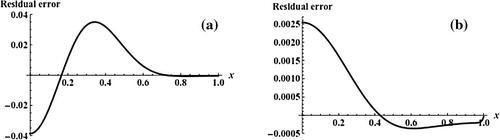
Using the software of Wolfram’s Mathematica, starting with u₀ (x,α), then, the successive approximations u_m+1 (x,α,h), m ⩾ 0, as followsand so on. With the help of the additional forcing condition (3.48)(3.48) , becomes(3.51) According to the Eq. (3.51)(3.51) , α as a function of the auxiliary parameter h has been plotted in the h-range [0,2] implicitly in Fig. 11. Two α-plateaus can be identified in this figure, namely α = 0.23 in the range [1.2,1.7] of h and α = 0.65 in the range [1.2,1.4] of h. To show the accuracy of these dual approximate solutions, we have shown the residual error R(x,α,h) (3.52)(3.52) for these solutions in Fig. 12.(3.52)

Figure 11 Plot α as a function of h at m = 6 in (3.51)(3.51) for the problem (3.45)(3.45) .

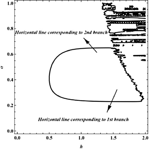
Figure 12 The residual error (3.52)(3.52) for the problem (3.45)(3.45) when h = 1.2. (a) The first branch and (b) the second branch.

4 Conclusions

The presented approach is proposed based on a variational iteration method with an auxiliary parameter not only to predict the existence of multiple solutions, but also to calculate all branches of solutions effectively at the same time. The most important advantage in this work is using a fixed iteration formula to predict the multiplicity of the solutions of nonlinear homogeneous ordinary differential equations with boundary conditions and using an auxiliary parameter, that provides us with a simple way to control the convergence region and rate of giving approximate series. The scheme is tested on four nonlinear practical differential equations. The results demonstrate reliability and efficiency of the algorithm developed.

Notes

Peer review under responsibility of University of Bahrain.