Differences in TFP growth among groups of dairy farms in the Netherlands

Abstract

The trend towards fewer and larger farms characterising agriculture in most industrialised countries can be partly attributed to larger farms becoming more productive by exploiting the economies of scale inherent in the production technology they employ. This paper examines whether larger and more intensive dairy farms in the Netherlands have been experiencing faster productivity growth than smaller farms, with the objective of determining which types of farms are more likely to prosper in the long run. Classification and regression trees are proposed as a valid way of classifying farms according to their size and farming intensity. At a second stage total factor productivity growth is calculated and decomposed into technical progress, efficiency change and scale effects for each class of farms using Data Envelopment Analysis. The results suggest that, for all classes of farms, productivity growth is driven almost exclusively by technical progress. The rate of technical progress has been higher for large intensive farms, implying that recent technical innovations are more beneficial to this type of dairy farms.

Keywords:

• dairy farming
• productivity growth
• farm size
• intensity

1 Introduction

The dairy sector in the Netherlands, as in most industrialized countries, has undergone major structural changes over the past decades. First, while half a century ago most farms produced an array of outputs, today they are highly specialised in the production of milk, with the bulk of grain feed bought in the market. Second, the number of dairy farms has been steadily declining, while the size of the farms that remain operational has been increasing. From an economic point of view, larger farms are possibly becoming more productive by exploiting the economies of scale inherent in the production technology. This, in turn, makes larger farms more competitive relative to the smaller ones, as they can produce more output per unit of input. Although the Netherlands is a country with a uniform climate, today's Dutch dairy farms are quite heterogeneous in terms of size. The 5% smallest dairy farms have less than 20 cows and have a gross margin as low as €54,000, whereas the 5% largest farms have more than 150 cows and their gross margin is larger than €318,000. From these differences in such a small country, a question rises naturally: are the trends towards fewer and larger farms going to persist? Furthermore, are benefits arising from economies of scale the only reason behind these trends?

The role of productivity growth is of major importance in answering these questions. Newman and Matthews [1] argue that differences in productivity growth rates is the main reason behind divergent trends in competitiveness. That is, if larger farms consistently experience faster productivity growth then, in the long run, they will become more competitive and, consequently, encourage smaller farms to adjust by expanding their scale or be driven out of business, with larger farms possibly acquiring their assets. Therefore, the evolution of productivity over time provides an indication of the development of relative competitiveness of different farming systems.

Before proceeding with the analysis we need an operational definition of productivity. In farming systems where individual farms use multiple inputs to produce multiple outputs, the definition of productivity is not straightforward. Total Factor Productivity (TFP) growth, defined as growth in outputs that cannot be attributed to growth in inputs, is the most widely accepted measure of productivity growth in such a setting. Apart from its ability to accommodate technologies where multiple inputs are used and multiple outputs produced, TFP growth encompasses the dynamic nature of the questions considered in this article.

TFP growth can be measured using different methods, each one of which has different data requirements and relies on alternative assumptions about the representation of the production technology and the ability of the farm manager to exploit the full potential of the technology. Simple Törnqvist indexes can be constructed using data on each farm in isolation of other farms in the sample, but under the assumption that every farm is technically efficient [2]. Two methods that explicitly recognize that farms may be inefficient in transforming inputs into outputs are Stochastic Frontier Analysis (SFA) and Data Envelopment Analysis (DEA). Since the introduction of SFA by Aigner et al. [3] and Meeusen and Broeck [4] this method has been widely applied. The other method was first proposed by Farrell [5] and extended by Seitz [6]. It presented a way of estimating a frontier production using linear programming techniques, but did not get wide acceptance until Charnes et al. [2] formalized it and coined the term Data Envelopment Analysis.

Both DEA and SFA compare multiple inputs with multiple outputs to measure efficiency and productivity and they can decompose TFP growth into three components: technical change, technical efficiency change and scale effect. Technical change results from a shift in the production technology. Technical efficiency comes from the farm's ability to use the available technology without wasting resources and the ability of a farm to use its inputs more efficiently and by operating closer to the technology frontier [7]. The last component, the scale effect, captures the effect on productivity of the ability of the farm to exploit economies of scale by modifying its size. The DEA method involves the use of linear programming methods to construct a non-parametric frontier over the data. Efficiency scores are then calculated relative to this frontier [7]. This frontier is not approximated by a production function as in the SFA method, but it is formed by dairy farms which produce the maximum possible amount of output with a given amount of inputs. Inefficient farms are projected onto the production frontier by using a convex combination of efficient farms (peers) that use similar input and output mixes [8].

Both methods available for calculating and decomposing TFP growth implicitly assume that all dairy farms share the same production technology. In our case, however, different types of farms could be employing alternative technologies, which are precisely the ones that are best-suited for them, given their size or other farm characteristics. Calculating TFP growth for all dairy farms would assume a common frontier, but if different types of farms employ alternative technologies this approach is not appropriate. The latent-class stochastic frontier approach [9] has been proposed in the literature as a way of dealing with this issue. However, the latent-class approach can be applied only in a parametric setting, i.e. when using SFA. Additionally, because the number of parameters to be estimated is a multiple of the number of assumed technologies, the latent-class framework becomes impractical in applications when the number of inputs and outputs considered is large. In this article we use instead a classification and regression tree (CRT) to distinguish classes. CRT's can divide the dairy farms in groups based on the technologies they employ and TFP growth can be calculated for each group of dairy farms which share the same technology using non-parametric techniques.

The aim of this study is to determine which types of farms are more likely to prosper in the long run based on the calculation of TFP growth. To achieve this objective the dairy farms are separated in groups in terms of the production technology they employ. The average TFP growth rate for each of these groups is calculated using DEA.

The rest of the paper is organised as follows. The next section presents the methodology used in this article. Section 3 contains a description of the data and section 4 presents and discusses the empirical findings. Finally, section 5 provides some concluding comments.

2 Methodology

Classification and Regression Trees (CRT) is a technique which can divide the farms in groups based on their characteristics. CRT splits the data into segments that are as homogeneous as possible with respect to the dependent variable. The most important difference between a classification tree and a regression tree is that classification trees use discrete and categorical dependent variables, whereas the dependent variable in regression trees is continuous. A CRT is essentially an algorithm for recursively splitting the dataset into two subsets which form the subtrees. The purpose is to maximise I[X;Y], where I is the information that the subtree provides, Y is the response variable and X _m , m = 1,….,M, are the predictor variables used to construct the purest possible subtrees [10]. Only univariate splits are considered which means that each split depends on the value of only one predictor value. A tree is grown according the following algorithm [11]:

1.	Find each predictor's best split: For each predictor, sort its values from the smallest to the largest. Go through each value of the predictor and determine the best splitting point as the one that maximises the splitting criterion (to be defined shortly) if the node is split according to it.

2.	Find the node's best split. Among the best splits found in step 1, choose the one that maximizes the splitting criterion.

3.	Split the node using its best split found in step 2 if the stopping rules are not satisfied. If a split takes place then repeat the previous steps for both of the resulting new nodes.

At node t, the best split s is chosen by maximising the splitting criterion:(1) $\Delta i(s,t)=i(t)-p_{L}i(t_L)-p_{R}i(t_R)$(1) where:(2) $i(t)=\frac{\Sigma n\in \hslash (t)fn{(yn-y(t))}^2}{\Sigma n\in \hslash (t)fn}$(2) with n as an index for the summation of Y, $\hslash (t)$ as the set of observations that fall in node t, f _n as the frequency weight associated with case n, where$p_L=N_W(t_L)/N_W)(t)\text{,}$ (4) $p_R=N_W(t_R)/N_W(t)$(4) with N _w (t) as the weighed number of cases in node t, N _w (t _L ) the number of cases which go to the left after splitting and N _w (t _R ) the number of cases which go the right after splitting.(5) $N_W(t)={\Sigma }_{n\in \hslash (t)}\cdot fn$(5) and(6) $\dot{y}(t)=\frac{\Sigma n\in \hslash (t)fn\cdot yn}{N_W(t)}$(6)

[11]. With this splitting criterion a tree with a high number of subtrees can be constructed, which may result in too many terminal nodes. It is possible that there are so many terminal nodes that the final tree overfits the data (rather than providing a representation of the population). To decrease the number of terminal nodes one can prune the tree. There are several criteria for impurity and the tree is grown until one of the criteria for impurity is met. The criterion that is used here is the minimum change in improvement of the tree. The improvement of a split is defined as:(7) $\Delta I(S^{*},t)=p(t)\Delta i(S^{\ast },t)$(7) where p(t) is the probability of a case being in node t. If for the best split s* of node t the improvement is smaller than the minimum improvement the node will not split. The default is 0.0001 and higher values tend to produce trees with fewer nodes [11].

After splitting the farms into homogeneous categories the average productivity growth per group of farms can be calculated. For this purpose the Malmquist TFP index can be used. This method was first introduced by Caves, Christensen and Diewert [12,13], who defined TFP index using Malmquist output distance functions. This approach resulted in an index which is known as the Malmquist TFP index. The technique starts from the definition of the distance function:(8) $d_o(x,q)=\min \{\delta :(q/\delta )\in P(x)\}$(8) where δ is the value of the distance function given a vector of inputs x, a vector of outputs q and the output-possibilities set, $P(x)=\{q:xcanproducey\}$. The distance function assumes values on the unit interval and it measures by how much a farm can equi-proportionally increase its outputs given a fixed amount of inputs. It is a representation of the multi-input, multi-output production technology which avoids specification of a behavioural objective [14].

Using the output distance function [12,13] define TFP growth between periods s and t as:(9) $m_o(q_s,q_t,x_s,x_t)=\frac{d^t(x_s,q_s)}{d^t(x_t,q_t)}$(9) where d ^t is the value of the distance function using the technology in period t. A value of the index greater than one indicates that productivity is higher in period s relative to period t, because more output is produced relative to the inputs used. Färe et al. [14] argue that one could equally well use the technology in period s as the reference and, to avoid making an arbitrary choice, they propose using the geometric mean of two productivity measures:(10) $m_o(q_s,q_t,x_s,x_t)={\left[\frac{d^t(x_s,q_s)}{d^t(x_t,q_t)}\times \frac{d^s(x_s,q_s)}{d^s(x_t,q_t)}\right]}^{0.5}$(10)

Further, [13] rewrite the last equation as:(11) $m_o(q_s,q_t,x_s,x_t)=\frac{d^s(x_s,q_s)}{d^t(x_t,q_t)}{\left[\frac{d^t(x_s,q_s)}{d^s(x_s,q_s)}\times \frac{d^t(x_t,q_t)}{d^s(x_t,q_t)}\right]}^{0.5}$(11)

In this formulation, the ratio outside the bracket measures the change in relative efficiency between periods s and t and is termed efficiency change. This term measures the distance to the production frontier of points observed in two time periods and using their respective technologies as reference. On the other hand, the term inside the bracket measures the pure effect of technical change as it compares the distance of observed input and output quantities in one period using the technologies in the two different periods as reference.

Finally, the efficiency change term can be further decomposed multiplicatively into pure efficiency change and the scale effect [14]:(12) $\frac{d^s(x_s,q_s)}{d^t(x_t,q_t)}=\frac{d_v^s(x_s,q_s)}{d_v^t(x_t,q_t)}\times \frac{d_c^s(x_s,q_s)/d_v^s(x_s{q}_s)}{d_c^t(x_t,q_t)/d_v^t(x_t{q}_t)}$(12) where $d_c^t$ is the distance function in period t imposing constant returns to scale on the production technology and $d_v^t$ allowing for variable returns to scale. The first ratio measures efficiency changes relative to the variable-returns-to-scale frontier and the second ratio measures changes in scale efficiency, or change in productivity due to farms adjusting their size.

For TFP growth indexes to be calculated and decomposed one needs values for all distances that appear in formulas (11) and (12). DEA is now used to calculate the values of the distance functions, that is, the distance of observed data points relative to the frontiers defining the technologies. DEA involves the use of linear programming methods to construct a non-parametric frontier over the data. Efficiency measures (values for of the distance functions) are then calculated relative to this frontier [7]. A major advantage of DEA is that it does not require any assumptions about the functional form of the production technology: the efficiency score of a dairy farm is measured relative to other dairy farms with the restriction that all dairy farms lie on or below the efficient frontier [15].

DEA can be applied under constant returns to scale (CRS) or variable returns to scale (VRS) such that all the values of the distance function that appears in (12) can be calculated. The difference between CRS and VRS is that in a situation of CRS output increases proportionally to increases in input, while, in case of VRS, output is more or less than proportionally increased compared to the increase in input. CRS can be applied when all farms are operating at an optimal scale but in practise, due to imperfect competition, government regulations, etc., farms are often not operating at an optimal scale. In that case it is more useful to apply VRS DEA which isolates the scale effect from overall efficiency change. In this research not all farms are operating at an optimal scale and, thus, VRS DEA will be applied.

To explain the linear programming problem it is best to first define some notation. Assume there are data on N inputs and M outputs for each of I farms. The i-th farm is represented by the input and output column vectors x _i and q _i , respectively. The N × I input matrix, X, and the M × I output matrix, Q, horizontally stack the data for all I farms [7]. The linear programming problem for VRS DEA can be defined as:(13) $\begin{array}{ll}Ma{x}_{\varphi ,\lambda }\varphi ,\hfill & \hfill \\ st:\hfill & -\varphi q_i+Q\lambda \ge 0,\hfill \\ \hfill & x_i-X\lambda \ge 0,\hfill \\ \hfill & I{1}^{\prime }\lambda =1\hfill \\ \hfill & \lambda \ge 0,\hfill \end{array}$(13) where ϕ is a scalar, λ is a Ix1 vector of constants and I1 is an I × 1 vector of ones. ϕ is greater than or equal to one and it indicates the proportion by which the observed output vector should be expanded such that it reaches the production frontier. For an efficient farm it ϕ is equal to unity and a measure of efficiency on the unit interval is obtained as the inverse of ϕ [7]. One can obtain the CRS DEA model by excluding the convexity restriction $I{1}^{\prime }\lambda =1$.

Scale efficiency measures can be obtained for each farm conducting both a CRS and a VRS DEA, and then decomposing the efficiency change obtained from the CRS DEA into pure efficiency change and scale efficiency change. If there is difference in CRS efficiency change and VRS pure efficiency change for a particular farm then this indicates that this farm is scale inefficient [7].

3 Data

This research used a database from the European Farm Accountancy Data Network (FADN). It includes Dutch dairy farms which are specialised in producing milk. This means that at least 50% of total revenues come from the production of cow's milk.

Results are presented for the period 1995 to 2000. This is a relatively short period but expanding the time period would be at the expense of the number of farms which are included in the dataset. This is because the FADN uses a rotating scheme which allows farms to remain in the panel for approximately 5-6 years.

The dataset includes 196 Dutch dairy farms and contains farm-level information on physical units (inputs and outputs), economic and financial data, some geographical characteristics and characteristics of the farm's primary operator [16]. The dataset is organised in five inputs and two outputs. The five inputs are:

1.

Capital; this includes buildings, fixed equipment, machinery and tractors and it is in terms of book value. Although FADN makes adjustments to the stock of capital for depreciation and market price changes, reappraisals are not performed entirely. Buildings and machinery are each deflated using their respective price indices before added together to form the aggregate capital variable. This measure represents the stock notion of capital, which, contrary to the flow notion (services of capital measured as depreciation plus opportunity cost) is less susceptible to short-term price movements.

2.	Labour; this includes own labour and hired labour and it is determined in annual full-time equivalents.

3.	Total utilised agricultural area (uaa); this includes owned land and land that is rented for more than a year and it is measured in hectares.

4.

Materials and services; this input is built up out of several components: seeds and plants, crop protection, fertiliser, livestock-specific costs, other costs, energy and feed. The costs for purchased feed and concentrates are included, but the value of feed which is produced in the farm is not included. Price indexes for each of these categories of expenditure, obtained from EUROSTAT, are used to construct an aggregate Törnqvist price index for total materials and services expenditures. Total materials and services costs are then deflated using this aggregate Törnqvist index.

5.	Livestock; this includes all animals on the farm during the year, both cattle and other animals. Different animals get different weights that are then added together to calculate the total livestock units defined by FADN.

The two outputs are:

1.	Revenues from milk production per dairy cow on the farm.

2.	All other output that is produced on the farm as well as changes in valuation for animals.

The reported revenues from both outputs are deflated using price indexes for each category of products. The price indexes are obtained from EUROSTAT. Physical units for the quantity of milk are available but information about the quality of the milk (fat and protein content) is not available. Instead revenues can reflect these quality differences because they include possible price premiums for higher quality. Therefore, deflated revenues are used as the measure of output in this study, implicitly taking into account quality differences.

Table 1 represents summary statistics of the data that are used for this paper. It includes the mean, standard deviation, minimum and maximum values of the outputs and inputs of the dataset. The economic size of the farms is an additional variable in the table and it is expressed in European Size Units (ESU). One ESU is €1200 of gross margin [17]. This means that the average size of a farm (123 ESU) has a total gross margin of €147,600.

Table 1 Summary of the data.

Variable	Mean	Std. Dev.	Min	Max
Cow's milk (× €1000)	154.5	89.2	20.1	591.8
Other output (× €1000)	35.1	33.6	2.5	263.6
Capital (× €1000)	253.2	154.5	31.3	1361.1
Materials and services (× €1000)	80.1	44.6	14.0	293.8
Total utilised land (ha)	39.4	22.1	9.6	170.7
Labour (fte)	1.7	0.6	0.7	3.7
Livestock (#)	108.7	61.6	25.2	400.4
Economic size (ESU)	123.0	68.8	22.5	450.3

4 Results and Discussion

Figure 1 presents the regression tree which divided the farms in groups. The dependent variable are the revenues from milk production per cow and the independent variables are the average size of the farms over the six years covered by the data and the average number of dairy cows per hectare. The dependent variable was chosen to reflect differences in the production technology by using the single most informative measure. The independent variables capture the effect of size and intensity on milk per cow.

Figure 1 Regression tree with revenues of milk production per cow (x €1000) as dependent variable and mean size (ESU) of the farms and number of dairy cows per hectare as independent variables.

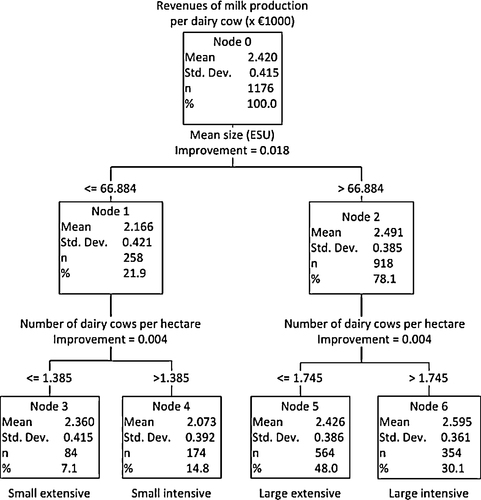
The tree divided the farms in two subsets based on their size first. The two subtrees became parent nodes and the tree divided the farms again in two subtrees, this time based on their intensity. Nodes 1 and 2 are produced by the first split. This first split divides farms into small and large. The cut-off point between small and large farms lies at, approximately, 67 ESUs. 918 of the 1176 observations (combined farm and time dimensions) are in the group with the large farms. This means that 153 farms are defined as large and 43 as small according to this regression tree. The 43 small farms are divided in two groups, node 3 and 4. These farms are divided on intensity with a cut-off of 1.385 dairy cows per hectare. There are 14 farms in node 3 which are small farms with a low intensity. Node 4 includes 29 farms which are small farms but have a higher intensity. The 153 farms in node 2 are also divided in two subtrees. Node 5 and 6 describe the intensity for the larger farms. The cut-off for these farms lies at 1.745 dairy cows per hectare. Node 5 includes 94 farms which are large farms but have a low intensity. The 59 farms in node 6 are large intensive farms. The intensity of the farms depends on the technology that they use. The cut-off between extensive and intensive farms lies 25% higher for large farms than the small farms. This makes sense because large farms are in better position to benefit from new technologies and increase their intensity: the average intensity of the large farms is 1.69 cows per hectare against 1.47 cows per hectare for small farms.

The first split, from the root node to node 1 and 2 has an improvement in change of the tree of 0.018. The minimum change in improvement is 0.0001 before a subtree is added so this split improves the accuracy of the tree and should be included. The improvements of the split from node 1 and 2 into the daughter nodes are 0.004 and 0.005 respectively. These values are above the minimum and are therefore valid. These values show that the accuracy of the tree grows when these nodes are added to the tree.

Table 2 presents the technical change effect for the years 1995-2000. It can be seen that the technical change is higher for large farms. Their annual change is 1.1% for the large extensive and 1.8% for the large intensive farms against 0.6% for the small extensive and 0.5% for the small intensive farms. This could be explained by the fact that larger farms are in better position to benefit from new technologies because they are easier to implement on a larger scale. The differences in technical change between extensive and intensive farms are smaller. The small extensive and small intensive farms have about the same technical change, which indicates that intensity does not influence the technical change that the small farms experience. The difference in technical change between large extensive and intensive farms is larger than for small farms. Additionally, the results suggest that large intensive farms are in better position to benefit from technical innovations than extensive farms.

Table 2 Technical change index for the years 1995-2000.

Years	Small extensive	Small intensive	Large extensive	Large intensive	All farms
	Technical Change
1995	1.000	1.000	1.000	1.000	1.000
1996	0.996	1.013	0.969	0.967	0.967
1997	1.056	1.062	1.016	1.045	1.031
1998	1.077	0.963	0.995	0.987	0.999
1999	1.084	1.052	1.106	1.122	1.113
2000	1.030	1.023	1.054	1.095	1.076
Annual	1.006	1.005	1.011	1.018	1.015

The technical change effect in 1998 is below one for every group except for small extensive farms. These low values are a remarkable observation because this would mean that technical regression took place in that year. An explanation for this technical regress could be the bad weather in that year. 1998 was the year with the most rain in that century. In June there was a lot of rain so farmers had difficulties in getting their grass in silage and had difficulties in letting their cows feed on the pasture. The months October and November were very wet as well, which caused problems with harvesting the maize and not all farmers were able to harvest all their maize.

Table 3 shows the pure efficiency change effect for the years 1995-2000. The differences between small and large farms are small. The large farms have a slightly higher efficiency change than the small farms. The annual pure efficiency change for the small farms is 0.0% for small extensive and -0.3% for small intensive farms. This indicates that small farms experience difficulties to increase their output with fixed inputs by operating closer to the technical frontier. The large extensive farms have an annual change of 0.2% and the large intensive farms 0.3%. These values are only slightly positive but higher than the efficiency changes of the small farms. These low changes would be expected because although there may be movement of individual farm scores from year to year, it is in generally not seen or expected that the average efficiency to change over time, mainly because technology changes and innovations are the main drivers of productivity.

Table 3 Pure efficiency index for the years 1995-2000.

Years	Small extensive	Small intensive	Large extensive	Large intensive	All farms
	Pure Efficiency change
1995	1.000	1.000	1.000	1.000	1.000
1996	0.997	0.988	1.006	1.018	1.003
1997	1.000	0.996	1.013	1.020	1.010
1998	0.987	0.979	1.008	1.014	0.992
1999	1.000	0.992	1.012	1.022	1.015
2000	1.000	0.987	1.010	1.017	1.009
Annual	1.000	0.997	1.002	1.003	1.002

Table 4 presents the scale effect for the years 1995-2000. As can be seen, the annual change is about the same for all four groups. The small extensive and small intensive farms have both an annual change of 0.2% whereas the large extensive and large intensive farms have an annual change of 0.1% and -0.2% respectively. These results show that all farms have difficulties with becoming more efficient by adjusting their size. This could be explained because it is difficult to adjust the size of the farm without influencing other inputs or outputs. When farmers want to maximise the output of cow's milk they have to acquire milk quota, which can be thought of as an additional input. It is therefore difficult to adjust the scale of the farm with increasing output without adjusting their inputs.

Table 4 Scale efficiency index for the years 1995-2000.

Years	Small extensive	Small intensive	Large extensive	Large intensive	All farms
	Scale Efficiency change
1995	1.000	1.000	1.000	1.000	1.000
1996	1.011	0.996	1.006	1.016	1.025
1997	0.992	1.024	1.011	1.009	1.026
1998	0.984	1.048	0.999	1.000	1.023
1999	1.010	1.019	1.010	0.995	1.008
2000	1.010	1.009	1.007	0.992	1.005
Annual	1.002	1.002	1.001	0.998	1.001

When looking at all three components, technical change is the component which drives the differences in TFP growth between small and large farms. The pure efficiency change and scale efficiency change are approximately equal for small and large farms. So it seems that technical change is an important component in becoming more productive. The differences between extensive and intensive farms do not become clear in these results, as no large differences between extensive and intensive farms are apparent in any of the components.

The results presented in this section are, in many respects, similar to those obtained in other studies of TFP growth in the dairy sector of European countries. For example, Emvalomatis [16] reports average TFP growth of 1.23% for dairy farms in Germany, with the technical-change effect contributing most of the productivity growth. Similarly, Newman et al. [1] found that TFP in Irish dairy farming grow at an average rate of 2.2% exclusively due to technical progress. Brümmer et al. [18] report considerably larger TFP growth rates for German and Dutch dairy farming: 6% and 2.9% respectively. Much of the difference could be attributed to the different and shorter time period spanned by their data (Brümmer et al. [18] consider the period 1991-94), although they still find that the main driver of TFP growth is technical change. Contrary to our findings, Alvarez and del Corral [19] find differences in TFP growth rates between intensive and extensive dairy farms in Spain: although intensive farms experience a TFP growth rate of 2.2%, extensive farms experience negative TFP growth due to adverse efficiency change and scale effects.

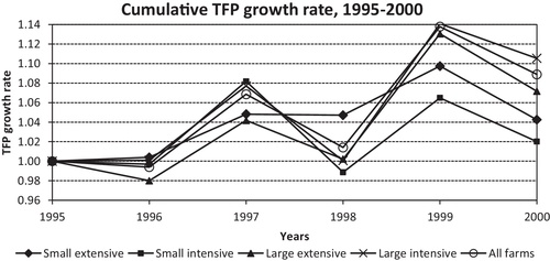
Figure 2 shows the cumulative TFP growth for the different groups of farms. 1995 is the base year and the value of the TFP index is normalized to 1 for all groups of farms. The large extensive farms have an annual TFP growth of 1.4% and the large intensive farms have an annual growth rate of 2.0%. These numbers are higher than the values for the extensive and intensive small farms, which have an annual growth of 0.8% and 0.4% respectively. The large farms have a higher cumulative TFP growth than the smaller farms so large farms increase their productivity at a higher rate than small farms. This means that small farms are getting behind on large farms and the difference between small and large farms will become larger. It seems that it does not matter whether a farm is extensive or intensive, TFP growth rates for extensive and intensive farms lie close to each other. 1998 shows a large decrease in TFP growth for all farms, this is probably due to the bad weather conditions as explained earlier in this section. It seems that this decrease only occurs for one year because in 1999 the TFP growth is up to a normal rate again.

Figure 2 The cumulative TFP growth rate for the farms from the first regression tree, based on the size and the intensity of the farm for the years 1995-2000.

5 Conclusions and Further Remarks

The objective of this study was to determine which types of dairy farms are more likely to prosper in a changing environment based on the calculation of TFP growth rates. To achieve this objective a sample of 196 dairy farms from the Netherlands were first separated in groups in terms of the production technology they employ. The regression tree method was used to accomplish this task and milk production per cow was chosen as an indicator for the technology that farms employ. Farms were divided in groups based on their size and farming intensity. The regression tree resulted in 4 groups of farms: small extensive, small intensive, large extensive and large intensive farms. In a second step, average TFP growth rates were calculated for every group of farms that resulted from the regression tree.

These results suggest an annual TFP growth rate for small extensive and small intensive farms of 0.8% and 0.4%, respectively. Large extensive and large intensive have a considerably higher annual TFP growth rate, 1.4% and 2.0%, respectively. The differences in TFP growth rates are much larger when considering different classes in the farm-size dimension rather than in farming intensity. For all four classes of dairy farms the technical-change component contributes the most in TFP growth. Technical change is faster for larger farms, suggesting that this type of farms benefited the most from recent technical innovations. The pure efficiency change and scale effects are small and approximately equal for all types of farms. The differences in the pure efficiency change and scale effects between groups of farms are, respectively, 0.6% and 0.3%. Small farms have the highest scale effect, implying that they are also becoming more productive over time by growing in size.

The findings of this study suggest that larger farms are more likely to prosper in the Dutch dairy sector. This is because they appear to be experiencing faster productivity growth over time and, therefore, any productivity gap between large and small farms is widening. On the other hand, what constitutes a “large” farm maybe changing over time. The regression tree used in this study split the farms at the point of 67 European Size Units (approximately €80,000 of standard gross margin), but even smaller farms in the sample seem to be becoming more productive by growing in size. If smaller farms start exiting the sector or becoming larger, this does not necessarily imply that the distribution of farm sizes will become more concentrated; it may rather shift towards larger sizes. In fact farms of vastly different sizes may continue to co-exist in the sector as it is the case in most industrialized countries, either because of slow adjustment or because of availability of certain resources (for example hired labour or access to credit).

Additionally, survival in a competitive environment is not determined solely by economic and technical results. Bergevoet [20], for example, showed that pleasure in work and minimizing risk are, next to technical results, examples of important factors for the development of a farm. Although financial success of a business is a key to survival, alternative objectives of family-owned farms may result in a slow-down of the trend towards fewer and larger farms.

References

- C. Newman A. Matthews Evaluating the Productivity Performance of Agricultural Enterprises in Ireland using a Multiple Output Distance Function Approach Journal of Agricultural Economics 58 1 2007 128 151
- A. Charnes W.W. Cooper E. Rhodes Measuring the efficiency of decision making units European Journal of Operational Research 2 6 1978 429 444
- D. Aigner C.A.K. Lovell P. Schmidt Formulation and estimation of stochastic frontier production function models Journal of Econometrics 6 1 1977 21 37
- W. Meeusen J.v.D. Broeck Efficiency Estimation from Cobb-Douglas Production Functions with Composed Error International Economic Review 18 2 1977 435 444
- M.J. Farrell The Measurement of Productive Efficiency Journal of the Royal Statistical Society. Series A (General) 120 3 1957 253 290
- W.D. Seitz The Measurement of Efficiency Relative to a Frontier Production Function American Journal of Agricultural Economics 52 4 1970 505 511
- Coelli, T.J., D.S.P. Rao, C.J. O’Donnell, and G.E. Battese, An introduction to efficiency and production analysis. Second ed. Springer science. 2005: Springer sciency + Business Media.
- T.J. Coelli A multi-stage methodology for the solution of orientated DEA models Operations Research Letters 23 3-5 1998 143 149
- S.B. Caudill Estimating a mixture of stochastic frontier regression models via the em algorithm: A multiproduct cost function application Empirical Economics 28 3 2003 581 598
- C. Shalizi Classification and regression trees Data Mining 2009 36 350
- Inc., S., SPSS classification Trees™ 13.0. 2004.
- Caves, D.W., L.R. Christensen, and W.E. Diewert, Multilateral comparisons of output, input and productivity using superlative index numbers. Economic journal, 1982. 92: p. 73-86.
- D.W. Caves L.R. christensen W.E. Diewert The economic theory of index numbers and the measurement of input, output and productivity Econometrica 50 1982 1393 1414
- R. Färe S. Grosskopf M. Norris Z. Zhang Productivity growth, technical progress and efficiency change in industrialized countries American Economic Review 84 1994 66 83
- L.M. Seiford R.M. Thrall Recent developments in DEA: The mathematical programming approach to frontier analysis Journal of Econometrics 46 1-2 1990 7 38
- G. Emvalomatis Productivity Growth in German Dairy Farming using a Flexible Modelling Approach Journal of Agricultural Economics 63 1 2011 83 101
- FADN. Field of Survey. 2012; Available from: http://ec.europa.eu/agriculture/rica/methodology1_en.cfm%23.
- B. Brümmer T. Glauben G. Thijssen Decomposition of Productivity Growth Using Distance Functions: The Case of Dairy Farms in Three European Countries American Journal of Agricultural Economics 84 3 2002 628 644
- A. Alvarez J. Corral Identifying different technologies using a latent class model: Extensive versus intensive dairy farms European Review of Agricultural Economics 37 2010 231 250
- Bergevoet, R.H.M., Entrepreneurship of Dutch dairy farmers, in Agricultural Economics Research Institute. 2005, WUR: Wageningen.