The effect of milk quota abolishment on farm intensity: Shifts and stability

Highlights

•	A mathematical programming model is applied to the Dutch dairy sector.
•	The milk quota abolition and associated policy measures are analysed.
•	The number of cows will increase for most of the farm types.
•	Only farms that are large in terms of Standard Output will become very intensive.

Abstract

We investigate whether milk quota abolition in the Netherlands is likely to lead to a shift towards more intensive farms, and whether the legislation introduced by the Dutch government to prevent this from happening is likely to be effective. To this end, a mathematical programming model is developed and applied to ten Dutch dairy farms of varying size. The mathematical programming model allows us to calculate shadow prices, which we use to evaluate the stability or likelihood of a shift in the farmer decisions in our model. Our results suggest a strong increase in intensity for the largest farm type when milk quotas are abolished, while further intensification is limited for the smaller farm types. Although most farm types increase the number of cows on the farm, for the smaller ones this can only be achieved when the costs of expanding decrease considerably. The new legislation introduced by the Dutch government to prevent strong intensification appears to be successful.

Keywords:

• Milk quota abolishment
• Farm intensification
• Shifts
• Manure
• Agricultural policy
• Netherlands
• Dairy farming

1 Introduction

Since 1984, the European Union (EU) has applied a supply quota for milk to prevent the overproduction that resulted from milk price support. This price support for milk was subject to critique, as it distorts global trade. In the 1990s, the World Trade Organisation urged the EU to abolish its system of price support [35,3], in response to which the EU decided to gradually liberalise its dairy policy. From 2003 onwards, support prices were reduced and the supply quotas were enlarged in steps. In recent years, world market prices for dairy products increased strongly, decreasing the gap between EU prices and world market prices. It is therefore that the EU has decided to abolish the supply quotas for milk completely [34], per 1st of April 2015 [18]. When production quotas such as those for milk are abolished, the industry structure (i.e. the number of farms and farm size distribution) is likely to be influenced [4,9,48], which may have important consequences for the land use and landscape in rural areas dominated by dairy farming, such as the Netherlands.

Table B1 Values of exogenous parameters.

parameter	description	value	parameter	description	value
w5	Yearly costs in € of growing a ha grass	1440	e10	kg P2O5 per KVEM from grass	0.01
w6	Yearly costs in € of growing a ha maize	1540	e11	kg P2O5 per KVEM from maize	0.005
w7	Costs of feed bought in € per KVEM	0.14	e12	kg P2O5 KVEM from feed bought	0.012
w8	Costs of removing P2O5 in € per kg	9.33	e13	kg P2O5 bound in 100 kg milk	0.222
w9	Costs of processing P2O5 in € per kg	10.83	e14	kg P2O5 bound in carrying cows	0.522
w10	Costs of hired labour in € per hour	16.74	e15	kg P2O5 bound in growth young cattle <1 year	4.619
w11	Yearly investment costs additional stable capacity including young cattle capacity in € per place for each extra cow	354.8	e16	kg P2O5 bound in growth cattle > 1 year	4.078
w12	Yearly costs of raising or buying extra cows in € per cow	294	e17	kg P2O5 allowed per ha grass land	95
w13	Yearly costs of renting extra land in euro	1200	e18	kg P2O5 allowed per ha maize land	65
e3	Share young cattle < 1 year per cow	0.64	e19	labour hours needed per 100 kg milk produced	0.5
e4	Share young cattle > 1 year per cow	0.29	e20	labour hours needed per ha grass land	7.2
e5	KVEM needed per cow	7197.8	e21	labour hours needed per ha maize land	7.0
e6	KVEM needed per young cattle < 1 year	1277.5	e22	hours of own labour available	7000
e7	KVEM needed per young cattle > 1 year	2555	e24	total ha land available for rent to farm n	20
e8	KVEM produced on 1 ha of grass land	11220	e25	maximum number of cows on farm	500
e9	KVEM produced on 1 ha of maize land	13720

Table B2 Values for the farm type specific exogenous variables in the reference year 2013.

Farm type	p2n = milk price in euros per 100 kg	e23n = initial ha land on farm n	e2n = initial number of cows on farm n	x1n = number of cows sold	w2n = Yearly maintenance costs in € per cow on farm n	e1n = milk production per cow in 100 kg	p1n = price of cows sold in euros per cow	hgin = initial ha grassland	hmin = initial ha grassland
Quantile 0–10	42.18	16	24	7	509	7291	774	15	1
Quantile 10–20	42.73	27	45	12	488	7548	696	26	1
Quantile 20–30	42.90	33	57	15	476	7692	671	32	1
Quantile 30–40	43.02	38	68	18	465	7822	653	37	1
Quantile 40–50	43.12	44	78	21	455	7945	639	43	1
Quantile 50–60	43.21	49	88	23	445	8068	627	48	1
Quantile 60–70	43.28	54	99	26	434	8199	616	53	1
Quantile 70–80	43.36	60	112	29	421	8347	605	59	1
Quantile 80–90	43.46	69	129	33	404	8554	592	68	1
Quantile 90–100	43.79	112	215	55	317	9594	544	111	1

Table C1 Model result farm gross margin in euros per farm type for the three policy options.

farm type/gross margin	PO1: Milk quota	PO2: No milk quota	PO3: Order of Council
Quantile 0–10	36306	36306	36306
Quantile 10–20	70999	73597	73459
Quantile 20–30	93229	97952	97952
Quantile 30–40	114926	124665	121631
Quantile 40–50	137106	152502	146225
Quantile 50–60	160498	179396	172451
Quantile 60–70	187064	207471	202533
Quantile 70–80	219254	238653	238653
Quantile 80–90	267371	280463	280463
Quantile 90–100	499098	585004	519508

Table C2 Model result number of extra cows that exceed initial stable per farm type for the three policy options.

farm type/extra cows that exceed initial stable capacity	PO1: Milk quota	PO2: No milk quota	PO3: Order of Council
Quantile 0–10	0	0	0
Quantile 10–20	0	26	25
Quantile 20–30	0	26	26
Quantile 30–40	0	101	31
Quantile 40–50	0	87	34
Quantile 50–60	0	73	37
Quantile 60–70	0	59	41
Quantile 70–80	0	42	42
Quantile 80–90	0	20	20
Quantile 90–100	0	285	61

Table C3 Model result processing costs in euro per farm type for the three policy options.

farm type/costs of processing phosphate	PO1: Milk quota	PO2: No milk quota	PO3: Order of Council
Quantile 0–10	0	0	0
Quantile 10–20	0	0	0
Quantile 20–30	0	0	0
Quantile 30–40	0	67632	5314
Quantile 40–50	0	55651	8697
Quantile 50–60	0	43902	11969
Quantile 60–70	0	31470	15379
Quantile 70–80	0	17473	17473
Quantile 80–90	0	0	0
Quantile 90–100	0	225621	34107

Table C4 Model result total hectare on farm per farm type for the three policy options.

farm type/ha land used	PO1: Milk quota	PO2: No milk quota	PO3: Order of Council
Quantile 0–10	16	16	16
Quantile 10–20	30	47	46
Quantile 20–30	38	53	53
Quantile 30–40	45	58	58
Quantile 40–50	51	64	64
Quantile 50–60	58	69	69
Quantile 60–70	65	74	74
Quantile 70–80	72	80	80
Quantile 80–90	83	89	89
Quantile 90–100	132	132	132

Table C5 Model result phosphate surplus in kg P₂O₅ per farm type for the three policy options.

farm type/phosphate surplus	PO1: Milk quota	PO2: No milk quota	PO3: Order of Council
Quantile 0–10	0	0	0
Quantile 10–20	0	0	0
Quantile 20–30	0	248	248
Quantile 30–40	0	6615	861
Quantile 40–50	0	5626	1290
Quantile 50–60	0	4657	1708
Quantile 60–70	0	3632	2146
Quantile 70–80	0	2480	2480
Quantile 80–90	0	905	905
Quantile 90–100	365	22879	5195

Table D1 Extra hectares of land rented per farm type for the three policy options.

Farm type/extra land rented	PO1: Milk quota	PO2: No milk quota	PO3: Order of Council
Quantile 0–10	−15	−15	−15
Quantile 10–20	−26	−26	−26
Quantile 20–30	−32	−32	−32
Quantile 30–40	−37	−37	−37
Quantile 40–50	8	8	8
Quantile 50–60	9	9	9
Quantile 60–70	11	11	11
Quantile 70–80	12	12	12
Quantile 80–90	14	14	14
Quantile 90–100	−29	−29	−29

Table D2 Number of cows per farm type for the three policy options.

Farm type/number of cows	PO1: Milk quota	PO2: No milk quota	PO3: Order of Council
Quantile 0–10	1	1	1
Quantile 10–20	2	2	2
Quantile 20–30	2	2	2
Quantile 30–40	2	2	2
Quantile 40–50	78	78	78
Quantile 50–60	88	88	88
Quantile 60–70	99	99	99
Quantile 70–80	112	112	112
Quantile 80–90	129	129	129
Quantile 90–100	133	133	133

Table D3 Cows per hectare per farm type for the three policy options.

farm type/number of cows per ha	PO1: Milk quota	PO2: No milk quota	PO3: Order of Council
Quantile 0–10	1.5	1.5	1.5
Quantile 10–20	1.5	1.5	1.5
Quantile 20–30	1.5	1.5	1.5
Quantile 30–40	1.5	1.5	1.5
Quantile 40–50	1.5	1.5	1.5
Quantile 50–60	1.5	1.5	1.5
Quantile 60–70	1.5	1.5	1.5
Quantile 70–80	1.5	1.5	1.5
Quantile 80–90	1.5	1.5	1.5
Quantile 90–100	1.6	1.6	1.6

Table D4 Shadow prices for stable capacity per farm type for the three policy options.

farm type/shadow price stable capacity	PO1: Milk quota	PO2: No milk quota	PO3: Order of Council
Quantile 0–10	0	0	0
Quantile 10–20	0	0	0
Quantile 20–30	0	0	0
Quantile 30–40	0	0	0
Quantile 40–50	0	57	57
Quantile 50–60	0	114	114
Quantile 60–70	0	175	175
Quantile 70–80	0	244	244
Quantile 80–90	0	341	341
Quantile 90–100	0	0	0

Within the Netherlands the abolishment of milk quotas has led to environmental concerns, as further intensification (i.e. number of livestock per hectare) is expected [39]. Such intensification is likely to lead to an increase in the amounts of nitrogen and phosphate produced, which poses a major threat to the fragile natural ecosystems that are − in the Netherlands − often spatially interwoven into the agricultural area. Soon after the introduction of the milk quota, the Dutch government issued regulations to protect the environment [23] limiting the amount of nitrogen and phosphate from manure and artificial fertilizer that can be put on the land. Excesses of nitrogen and phosphate were to be removed from the farm [8], which led to a considerable trade in these excesses, among agricultural sectors and even with other countries. To prevent even larger excesses due to quota abolishment (the ceiling for the application of phosphate on land has remained unchanged), an additional law, referred to as the “Wet verantwoorde groei melkveehouderij” (law to ensure responsible growth of the dairy sector) or “Dairy law” (in Dutch Melkveewet), has been introduced in January 2015. Any phosphate surplus in excess of the amount prior to the milk quota abolishment has to be processed [17], meaning considerable extra costs for the farmer.

Yet, more restrictions were deemed necessary. Although the Dairy law addresses environmental concerns by regulating potential phosphate surpluses, it still allows farms to grow and/or intensify. Intensive dairy farming has become a topic of societal debate for various reasons. Firstly, it is associated with cows that remain permanently indoors, which is considered to result in a loss of cultural ecosystem services (meadows with cows are considered esthetically pleasing) [54]. Secondly, animal welfare is considered to be at stake in high-intensity farms, also due to the fact that many cows never leave the stable [44,47]. Thirdly, many people consider the existence of very large farms (and large stables in particular) undesirable. Most people associate farming with family farms, and oppose the idea of industrialization of farming [27]. Whether or not these arguments are justified, the ministry of Economic Affairs accommodated them by implementing a further measure (i.e. the ‘Order of Council’) in September 2015 that imposes a restriction on the intensification of Dutch dairy farms [40]. The measure specifically ensures land-based growth by demanding that – for intensive farms – further increases in the on-farm phosphate surpluses are only allowed when a certain amount of land is available [38,40]. This means that most farmers who want to increase their dairy herd can only do so if they purchase additional farmland.

The objective of this paper is to investigate whether the abolition will lead to a shift towards larger and more intensive farms in the Netherlands. In addition, we explore the effectiveness of the Order of Council. We do this for a range of farm sizes, as we expect that responses to policy changes will differ strongly per size category. More specifically, we expect that large farms are more likely to intensify when milk quotas are abolished than small farms. This is because larger farms have higher economic and environmental efficiencies [7], have lower per-unit production costs, and are therefore more likely to invest in more animals. Taking into account this variability within the farm population is thus essential to reveal the potential impact of policy reforms.

A mathematical programming model is developed and applied to ten representative Dutch dairy farms of different size as measured by Standard Output (SO). SO is the average monetary value of the agricultural output at farm gate price, and is considered a good measure of the economic size of a farm [19]. The model is used to analyse the likelihood of a shift towards a more intensive farm. We formulated three policy options: one reflects the situation with the milk quota still in place, the second reflects the situation in which milk quotas are abandoned but the Order of Council is not in effect, and the third captures the situation in which the Order of Council is introduced. Section 2 provides a short background. Section 3 discusses the methods we use. The results are presented in Section 4. Section 5 provides a sensitivity analysis and Sections 6 and 7 provide the discussion and conclusion.

2 Background

Agricultural land takes up about half of the total surface area in the Netherlands [13,14] and about 40 percent of agricultural land is used by dairy farms [10]. The majority of Dutch dairy farms is specialised in milk production [52]. In 2014 there were around 17,000 dairy farms in the Netherlands [10] which had an average SO of 339,000 euro. An average Dutch dairy farm as described by the Farm Accountancy Data Network (FADN) has 50 ha of land and 90 dairy cows, which comes down to an average intensity of 1.8 cows per ha in 2014 [29]. Considering an average phosphate production of 45.5 kg per cow, and an allowed application rate of 95 kg phosphate on grassland [8], 1.8 cow per ha would not require any manure to be exported off-farm. However, since most farms also apply artificial fertilizer, and keep young cattle which are not included in the average of 90 cows as recorded in the FADN, most dairy farms export or process manure. In 2014, 85.6 million kg of phosphate [50] and 257 million kg of nitrogen [15] was produced by dairy farms. The Dutch government has made an agreement with the European Commission that allows farms to apply an additional amount of nitrogen to their land when at least 80 percent of their land is grassland. This is referred to as derogation and in exchange for the increased application of nitrogen allowed by the European Commission the Dutch government has to ensure that the total amounts of nitrogen and phosphate from manure stay below a so-called phosphate and nitrogen ceiling [50]. In 2014 77% of the dairy farms had an excess of phosphate that had to be exported from the farm or processed [15]. If we consider the whole agricultural sector 172 million kg phosphate was produced of which 137 million kg could be applied on land, 28 million kg was exported to other countries, and 10 million kg was processed [16].

As for the other issues around farm size and intensification, 69% of all dairy farms allow their cows to graze outside [11]. Within the Netherlands there is a general trend towards increasingly larger farms. This trend is also visible for the Dutch dairy sector. The number of farms with more than 250 cows has increased from 44 in 1980 to 355 in 2015. From 2011 onwards, the number of dairy farms in the Netherlands has decreased, while the number of dairy cows has increased. Thus, more cows are kept on bigger farms [12].

3 Method

3.1 Mathematical programming

Mathematical programming is a method for identifying an optimal allocation of resources [31]. Within a mathematical programming model, an objective function is specified, which is maximized or minimized given a set of constraints. In this paper we assume that farms’ main goal is to optimize their gross margin or profit. The assumption of profit maximization is in line with assumptions that are generally made in economic modelling [36], although it should be mentioned that in reality farms might have other objectives such as the minimization of labour use and risk or the environmental impact of farming as well [45,1,43,53]. Mathematical programming allows us to study changes in the optimal farming decisions, which are the result of constraints becoming more or less binding.

In our model a farm maximizes gross margin given a set of technological and institutional constraints. These constraints can be both equality and inequality constraints. The basic structure of a mathematical programming model with only technological and inequality constraints is given in Eq. (1(1) ${\displaystyle \underset{x_i}{\max }}Z={\displaystyle {\displaystyle \sum }_{i=1}^N}\left(p_i{x}_i-w_i{x}_i\right)$(1) ).(1) ${\displaystyle \underset{x_i}{\max }}Z={\displaystyle {\displaystyle \sum }_{i=1}^N}\left(p_i{x}_i-w_i{x}_i\right)$(1) subject to:(1a) ${\displaystyle {\displaystyle \sum }_{i=1}^N}{a}_{ik}{x}_i\le b_k{\forall }_k\left[{\pi }_k\right]$(1a) (1b) $x_i\ge 0{\forall }_i$(1b) where: $Z$ is gross margin defined as total revenues minus total variable costs, $p_i$ refers to revenues per unit of activity i, $w_i$ is the variable costs per unit of activity i, $x_i$ is the level of activity i, $b_k$ is the total availability of a resource k, $a_{ik}$ is the quantity of resource k demanded by activity i, and ${\pi }_k$ is the shadow price of input k.

Eq. (1(1) ${\displaystyle \underset{x_i}{\max }}Z={\displaystyle {\displaystyle \sum }_{i=1}^N}\left(p_i{x}_i-w_i{x}_i\right)$(1) ) states that farms maximize gross margin by choosing the optimal activity levels under the assumption of exogenous output and input prices. Optimization takes place according to two types of restrictions. First, restriction 1a gives inequality restrictions, for example that the total use of fixed inputs should be less than or equal to the endowments of these inputs. Second, restriction Eq. (1b(1b) $x_i\ge 0{\forall }_i$(1b) ) states that activity levels cannot be negative.

3.2 Stability, regime shifts and shadow prices

Models such as the one developed here, are commonly used to identify the optimal allocation of a set of resources under specific conditions and constraints. Their static nature does not – at first sight – qualify them for exploring temporal dynamics. However, we do think they can be used to reveal a potential disposition of a system for regime shifts. This is because these models typically reveal non-linear responses of system properties (i.e. the resource allocation that leads to the highest profit) to prices and availability of the resources. The non-linear relationship between the availability of a factor and the optimal allocation of resources is the result of multiple factors that are potentially binding.

If a mathematical programming model contains only two factors that influence the objective we can give a graphical presentation of the optimization problem (Fig. 1).

Fig. 1 Graphical representation of the optimization problem, based on [25].

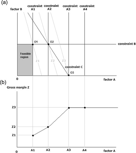
Panel (a) shows the two factors A and B that can be combined to reach a certain gross margin level Z. In the initial situation constraint A1, B and C are given, and all choices for the levels of A and B that are feasible form the feasible region. In the initial situation the feasible region is determined by the binding constraints A1 and B, while constraint C is not binding. The light grey lines labelled Z are the iso-profit lines. These lines connect all the combinations of factor A and B for which the profit reaches the same level. In the initial situation the highest level of gross margin that can be obtained is Z1, where point O1 indicates the optimal amounts of factor A and B used in this case. Now imagine one more unit of factor A would become available, shifting the constraint from A1 to A2. This would mean that the feasible region grows and the highest level of gross margin that can now be obtained is Z2. The point O2 indicates the optimal amounts of factor A and B used in this case. The difference between Z1 and Z2 is the extra gross margin that results from having one more unit of factor A available, which is referred to as the shadow price of factor A. If the decision maker would have the opportunity to obtain an extra unit of factor A, the shadow price would be the maximum amount the decision maker would be willing to pay to do so. If we shift to constraint A3, constraint C, which was previously not binding the optimal solution, now restricts the optimal level of gross margin that can be obtained. The point O3 indicates the optimal amounts of factor A and B used in this case. Shifting the constraint even further out to A4 would no longer result in extra gross margin, since constraint C prevents this. In Panel (1b) we show the response of gross margin to an increase in the availability of factor A, if we keep all other constraints fixed. Whenever binding factors change (i.e. the lines representing constraints in Panel (1a) change), the optimal solution and its associated resource allocation changes as well, but not in a linear way (Panel (1b)): As long as binding factors are relaxed or changed, the optimal solution will change as well; but once another constraint ‘takes over’ the binding role, the optimal solution will no longer respond to changes in the (now no longer binding) factor.

Hence, it is possible that the optimal solution does not change when we change the value of one of the constraints (say from A4 to A3 in Panel (1b)), but when we continue changing the constraint value, at some point (A3) a small extra change will be enough to result in a different optimal solution. This is a clear analogy with the concept of regime shifts as proposed by [20]. Following this analogy, optimal solutions can be seen as domains of attraction, the range over which a constraint can change without affecting the optimal solution can be seen as resilience, while the shift from one optimal solution to another could be seen as a regime shift. Although in this case the regime shift does not result from complex system behaviour (e.g. interactions between individual building blocks, and feedbacks between scale levels), and the shift itself is not characterized by an (uncontrollable) cascade of positive feedbacks, there is a clear non-linear response that needs to be accounted for when anticipating the effects of a policy measure. In a mathematical programming model the stability or resilience of the optimal solution can be measured by its relative position within the range of optimality. This range indicates the maximum change that the system can absorb due to a change in a driver (e.g. the amount of manure that has to be processed) without changing the optimal solution [25].

Since a graphical representation is only possible in the case with two constraining resources (and we have many more), a useful indicator for the degree to which a factor is binding, is the shadow price. A shadow price indicates what the value is of one more unit of a resource to the decision maker [21]. For example, if a farm is constrained by the initial stable capacity (factor A) the shadow price indicates how much a farmer would be willing to pay to increase the stable capacity (shifting constraint A). If the shadow price is zero, the stable capacity is not constraining the production. If the shadow price is positive, but less than the actual investment costs, the farmer will not be willing to invest. Only when the shadow price equals or exceeds the investment costs the farmer would start investing in extra stable capacity. Hence, shadow prices allow us to quantify the likelihood of a shift in one of the constraints, and thus the optimal solution. We will use these concepts to interpret our results in terms of the likelihood of a shift or stability.

3.3 Model

Our model describes the decisions made by Dutch dairy farms. It is assumed that a farm maximizes gross margin given a set of constraints. Gross margin is the result of revenue from milk production and selling cows that are no longer suited for milk production against a fixed price, minus the maintenance costs of cows and young cattle, the costs of growing grass and maize, the costs of buying feed, the costs of removing phosphate (P₂O₅), the costs of processing phosphate (which is higher than the costs of removing phosphate), the costs of hiring additional labour, the investment cost in additional stable capacity, the costs of raising or buying extra cows and the cost of renting extra land to a maximum of 20 ha. It is possible that the farm rents out some of its initial land, in which case the costs of renting extra land are negative and result in extra revenue. A mathematical presentation of our model can be found in Appendix A.

The farm is restricted by its initial endowment of land, cows, stable capacity, own labour and policy regulations. There is a policy which limits the amount of phosphate that can be placed on land. In the situation where milk quotas are applied policy restricts the amount of milk that can be sold. In the case where milk quotas are abandoned and the Dairy Law is introduced policy restricts the amount of phosphate that can be removed. In the case where milk quotas are abandoned and the Order of Council is introduced policy dictates a certain amount of land that needs to be bought when expanding production.

In our model there are three shadow prices of interest. First, the shadow price that indicates the value of extending the initial stable capacity with one more cow. This is relevant as we assume that there is a maximum farm size in terms of cow numbers (i.e. 500 cows) and the farm will only extend stable capacity when the shadow price is equal or higher than the yearly investment costs of additional stable capacity. Second, the shadow price indicating the value of one more hectare of land the farm can rent. This is relevant as we assume a farm cannot extend with more than 20 ha and the farm will only attract extra land if the shadow price is higher than the costs of renting extra land (1200 € per ha). Third, the shadow price indicating the value of having one more hour of labour available. This is relevant as below an external wage (16.74 € per hour) a farm will not hire external labour. Our model provides a more simplified and stylized version of a mathematical programming dairy model than for instance the model of Berentsen and Giesen [2], to allow a stronger focus on the possibility of a shift.

Our model allows farms to rent up to 20 ha of extra land, paying 1200 € per hectare. Farms can increase the number of cows up to 500, which we consider to be the maximum number of cows that can still be managed on a family farm. Each farm has 7000 h of own labour available, more labour from outside the farm can be hired, for which the farm pays a wage of 17 € per hour. As mentioned before we present all results compared to the initial situation in the BIN data set.

3.4 Data

The costs of feed bought, the costs of removing phosphate, the costs of maintaining young cattle, the costs of extra cows, the yearly investment costs in the stable, the costs of hired labour, the amount of feed measured in KVEM (measure for energy content of feed) produced on a ha of grassland and maize land, the amount of young cattle needed for replacement of current dairy cows, the amount of phosphate allowed on a ha of grassland and maize land, and the percentage grassland needed to be able to apply for derogation are taken from the Quantitative Information Livestock Industry report KWIN 2014–2015 [8]. The KVEM needed per cow, the KVEM needed for young cattle, and the amount of own labour hours available are taken from the handbook on the dairy farm sector 2014 [37]. The kg P₂O₅ per KVEM from grass, the kg P₂O₅ per KVEM from maize, the kg P₂O₅ per KVEM from feed bought, the kg P₂O₅ bound in milk, kg P₂O₅ bound in carrying cows and kg P₂O₅ bound in young cattle are taken from the assistance report for calculating phosphate production on dairy farms by the Dutch government. The labour hours needed for milk production, for cultivating grass land and for cultivating maize land are taken from [32], the land rent is based on [5] and the costs of cultivating a ha grass land and maize land are calculated using the “Kostenwijzer voedermiddelen” (Cost indicator for feedstuff) [51].

To be able to discuss the effect of milk quota abolition we defined 10 farm types based on SO, describing farms with increasingly larger SO. Our starting point in creating these different farm types was the BIN dataset [29]. This dataset provided us with information on the total farm area, the initial number of cows, the number of cows sold, the production per cow, the price of cows sold and the other costs of keeping cows for three different farm sizes.

The data from BIN provided us with the opportunity to calculate the percentage of the total farms represented by each of the three farm types based on SO. In 2013, a 0.1 share of the farms fell in the category 0–150,000 SO, a 0.2 share of the farms fell within the category 150,000–250,000 and a 0.5 share of the farms fell within the 250,000–500,000 category. These shares do not add up to one, since there are farms that fall in the category larger than 500,000. Using this information we searched for a distribution that fitted our data and that we could calibrate to our data. We considered a normal distribution, a gamma distribution and a Weibull distribution. The distribution that we found fitted our data the closest was the Weibull distribution. The probability density function of a Weibull distribution has the following form:$f\left(t\right)=\left(\frac{a}{B}\right){\left(\frac{t}{B}\right)}^{a-1}\times e^{\left[-{(\mathrm{t}/\mathrm{B})}^a\right]}$

This distribution is positively skewed if the value of a is smaller than 3.6 [28]. The distribution we use is described by Eq. (2(2) $x_{2n}={\displaystyle \overline{e_{2n}}}+x_{12n}-x_{1n}$(2) ).(2) $f\left(x\right)=\left(\frac{2.12}{439}\right)\times {\left(\frac{x}{439}\right)}^{1.12}\times e^{-{(x/439)}^{2.12}}$(2) where: $x$ size in 1000 SO.

We then divided this distribution in intervals, looking at the SO of farms at the 10, 20, 30, 40, 50, 60, 70, 80 and 90 percent quantile. To present each group we took the average of SO of the farms at the beginning and end of each interval. For example, for the farm type in the 0–10 percent quantile SO was the average of SO at the 0 percent quantile and SO at the 10 percent quantile. In this way 10 farm types based on SO were created which each present an equal share of the farms.

The next step was to calculate the value of the exogenous variables that are used in the model. In order to do this the farm size in terms of SO was plotted against each exogenous variable. Using the three data points a trend line was fitted to the data. The resulting equation was then used to estimate the values of the exogenous variables for the different farm types.

The decisions made by the farm are influenced by policy, input prices and output prices. The values of the exogenous prices in the model can be found in Table 1. Some values differ between the different farm types in which case a price range is given, while others are the same for everyone. A further description of the data used in our model can be found in Appendix B. Data were taken for the period 2013–2014.

Table 1 Values for the prices and costs used in the model.

Price	Value
Yearly maintenance costs in € per cow on farm n	234–509
Yearly maintenance costs in € per young cattle on farm n	45–97
Yearly costs in € of growing one ha grass	1440
Yearly costs in € of growing one ha maize	1540
Costs of feed bought in € per KVEM	0.14
Costs of removing P2O5 in € per kg	9.33
Costs of processing P2O5 in € per kg	10.83
Costs of hired labour in € per hour	16.74
Yearly investment costs additional stable capacity including young cattle capacity in € per place for each extra cow	354.80
Yearly costs of raising or buying extra cows in € per cow	294
Yearly costs of renting extra land in € per ha	1200
Price of cows sold from the farm in € per cow for farm n	515–770
Milk price in € per 100 kg	42.18–43.78

3.5 Policy options

We ran our model for the following three policy options:

3.5.1 PO1: milk quotas

This policy option fits the situation before 1 April 2015. In this policy option, the farm maximizes gross margin but is constrained by the milk quota, which limits milk production and thus the number of cows.

3.5.2 PO2: milk quotas abolished, no Order of Council

In this policy option, the farm maximizes gross margin, and is no longer constrained by the milk quota. The number of cows on the farm is now only limited by a supposed maximum amount of 500 cows that can be managed by a family farm; this assumption is based on [49,22,6]. Any phosphate surplus in excess of the amount that already was exported off-farm prior to the milk quota abolishment in the reference year 2013, has to be either processed (against a considerable cost), applied on land (but up to limited amounts per hectare), or a combination of these two measures.

3.5.3 PO3: milk quotas are abolished and Order of Council is introduced

In this policy option, the farm maximizes gross margin and is no longer constrained by the milk quota. However, the Order of Council is introduced, ensuring land-bound growth. Farms that have a phosphate surplus below 20 kg phosphate per hectare are excluded from the Order of Council and any phosphate surplus in excess of the amount that already was exported off-farm prior to the milk quota abolishment in the reference year 2013 has to be either processed, applied on land, or a combination of these two measures. If the farm has an on-farm phosphate surplus above 20 kg phosphate per hectare, a certain share of this has to be placed on additional land. Farms that have a phosphate surplus between 20 and 50 kg per hectare are obliged to place 25 percent of the additional phosphate production on land and farms that have a surplus above 50 kg per hectare are required to place 50 percent of the additional phosphate production on land, the rest of the additional phosphate surplus can be either processed, applied on land or a combination of these two measures.

Note that PO1 in a way reflects the situation of the recent past, which could allow us to use existing data rather than model outcomes. However, the initial situation as presented by the BIN data might not be the gross margin maximizing situation. In the model we allow for an increase in the amount of land rented and in the stable capacity on the farm, which is, in reality not always that simple, due to scarcity of land or the requirement to obtain building permits. To capture this we compare the results from the three policy options with the actual situation as described by the BIN data.

4 Results

Table 2 shows the amount of extra land rented by the 10 farm types for the three policy options (PO). The farms in quantile 0–10 present the farms with the smallest SO and the farms in quantile 90–100 present the farms with the largest SO. The smallest farm type rents out one hectare of land for all policy options. With the number of cows on this farm no additional land is needed for placing a phosphate surplus. The other farm types rent some extra land under PO1, as it provides them with feed and the option to put phosphate on land. The number of cows under PO2 is higher than under PO1, leading to a higher demand for land as well. Under PO2 Farm types in the 10–100 percent quantiles rent all available extra land (i.e. up to 20 ha, see Section 3.3). Under PO3 this is largely the same, but somewhat lower for the farm type in the 10–20 quantile, who has a slightly lower number of cows in this policy option.

Table 2 Extra hectares of land rented per farm type for the three policy options.

Farm type/extra land rented	PO1: Milk quota	PO2: No milk quota	PO3: Order of Council
Quantile 0–10	−1	−1	−1
Quantile 10–20	3	20	19
Quantile 20–30	5	20	20
Quantile 30–40	6	20	20
Quantile 40–50	8	20	20
Quantile 50–60	9	20	20
Quantile 60–70	11	20	20
Quantile 70–80	12	20	20
Quantile 80–90	14	20	20
Quantile 90–100	20	20	20

Table 3 shows that the number of cows for all but the smallest farm type is higher under PO2 and PO3 compared to PO1, but less so under PO3 than in PO2. Increase in cows is constrained by different factors for different farm size types. Farm types in the 10–30 percent quantiles would – under PO2 – have to start paying for the removal or processing of excess phosphate when increasing the number of cows any further, while farm types in the 30–90 percent quantiles use all of their own labour, so that increasing the number of cows would result in more hired labour costs. Since the costs outweigh the extra gross margin, these farms will not expand their number of cows any further. Since the larger farm types have a larger initial endowment of land, they end up with more land than the smaller farm types. For the farm types limited by the availability of own labour the consequence is that more labour is spent cultivating land and less labour is available for the cows, explaining the decreasing number of cows with increasing farm size for those farms in the 30–90 quantiles of PO2. The number of cows is lower in PO3 for all farm types in the 10–100 percent quantiles than in PO2.

Table 3 Number of cows per farm type for the three policy options.

Farm type/number of cows	PO1: Milk quota	PO2: No milk quota	PO3: Order of Council
Quantile 0–10	24	24	24
Quantile 10–20	45	71	69
Quantile 20–30	57	83	83
Quantile 30–40	68	168	99
Quantile 40–50	78	165	112
Quantile 50–60	88	161	126
Quantile 60–70	99	158	140
Quantile 70–80	112	154	154
Quantile 80–90	129	149	149
Quantile 90–100	215	500	276

As a measure of intensity Table 4 presents the number of cows per hectare under the different policy options for the ten farm types. The number of cows per hectare for the farm types in the 0–20 percent quantiles is not affected by the policy options. Even though the farm types in the 10–20 percent quantile increase their number of cows, they increase the amount of land accordingly. The farm types in the 10–100 percent quantiles all rent extra land under PO2 and PO3. PO3 is effective in terms of avoiding intensification for the farm types in the 30–70 and 90–100 quantiles as it results in a lower number of cows per ha. The farms in the 30–90 quantiles use all of their own labour available, limiting the total number of cows. Because larger farms have a larger initial land endowment, and because all farms in the 30–90 quantiles rent all available extra land when milk quotas are abolished, the number of cows per ha decreases when the farm size measured in SO increases under PO2.

Table 4 Cows per hectare per farm type for the three policy options.

farm type/number of cows per ha	PO1: Milk quota	PO2: No milk quota	PO3: Order of Council
Quantile 0–10	1.5	1.5	1.5
Quantile 10–20	1.5	1.5	1.5
Quantile 20–30	1.5	1.6	1.6
Quantile 30–40	1.5	2.9	1.7
Quantile 40–50	1.5	2.6	1.8
Quantile 50–60	1.5	2.4	1.8
Quantile 60–70	1.5	2.1	1.9
Quantile 70–80	1.5	1.9	1.9
Quantile 80–90	1.5	1.7	1.7
Quantile 90–100	1.6	3.8	2.1

Table 5 shows that the phosphate surplus per hectare is larger for the farm types in quantiles 20–100 under PO2 and PO3 compared to PO1. Under PO2 and PO3 farm types 20–90 rent all extra land that is available. Larger farm types have a larger initial land endowment and a smaller number of cows due to the restriction on own labour available. This explains how larger farm types can have a smaller surplus per hectare. PO3 effectively lowers the phosphate surplus per hectare for farm types in the 30–70 and 90–100 quantiles.

Table 5 Phosphate surplus per ha per farm type for the three policy options.

farm type/phosphate surplus per ha	PO1: Milk quota	PO2: No milk quota	PO3: Order of Council
Quantile 0–10	0	0	0
Quantile 10–20	0	0	0
Quantile 20–30	0	5	5
Quantile 30–40	0	113	15
Quantile 40–50	0	89	20
Quantile 50–60	0	68	25
Quantile 60–70	0	49	29
Quantile 70–80	0	31	31
Quantile 80–90	0	10	10
Quantile 90–100	3	173	39

The results show that the differences between farm types in costs and revenues in the model are determining the outcomes. Since small farms have higher maintenance costs per cow and a lower production per cow they are less likely to become big and very intensive when milk quotas are abolished. Only the largest farms found in the 90–100 percent quantile will increase the number of cows per hectare under PO2 significantly, since they can afford to pay the investment costs in stable capacity, the hired labour costs, the rent for extra land, and the costs of processing phosphate. More model results for the gross margin per farm type, the number of cows exceeding initial stable capacity per farm type, the phosphate processing costs per farm type, the hectares per farm type and the phosphate surplus per farm type can be found in Appendix C.

4.1 Stability and shifts within the model

Table 6 shows the shadow prices for stable capacity for the different farm types in the different policy options. The shadow price for stable capacity indicates the extra gross margin a farm could achieve when having one more place in its initial stable capacity. If this amount is equal to the costs of investing in one more stable place (355 euro) the farm will choose to do so and there is no limit to the amount of extra stable places a farm can invest in. The shadow price tells us how far the price of stable capacity would have to go down for the farms to start investing in additional stable capacity. The shadow price can therefore be seen as an indicator for the distance to a tipping point where farms will no longer be kept from expanding due to the investment costs in stable capacity. Table 6 shows that this situation is reached for all farm types under PO2 and PO3 except the 0–10 quantile.

Table 6 Shadow prices (€ per cow) for stable capacity per farm type for the three policy options.

farm type/shadow price stable capacity	PO1: Milk quota	PO2: No milk quota	PO3: Order of Council
Quantile 0–10	0	276	276
Quantile 10–20	0	355	355
Quantile 20–30	0	355	355
Quantile 30–40	0	355	355
Quantile 40–50	0	355	355
Quantile 50–60	0	355	355
Quantile 60–70	0	355	355
Quantile 70–80	0	355	355
Quantile 80–90	0	355	355
Quantile 90–100	0	355	355

Under PO2 and PO3 only the smallest farm type in quantile 0–10 is constrained by the investment costs in extra stable capacity. The shadow price shows that these costs would have to go down considerably before this decision would change and a shift towards investment in extra stable capacity would occur. Therefore the choice made by the farm type in the 0–10 quantile is quite stable with respect to investment costs for stable capacity. The other farm types are not constrained by the stable capacity (as under PO1) or the investment costs in stable capacity (as under PO2 and PO3).

The shadow price for land as presented in Table 7 measures what it would be worth to the farm if there would be 1 more ha of land that it could rent. Under PO2 all farms except those in quantile 0–10 and under PO3 all farms except those in quantile 0–20 rent the maximum allowed 20 ha (see Table 2). If the maximum amount of extra land available for rent to the farm is not constraining its production, the shadow price for extra land available for rent is 0. The shadow price is zero when the gross margin increase (excluding the costs of buying land) of buying land is less than 1200 euros (i.e. the price of buying land) making the net gross margin increase of renting land negative. So the farm does not buy land and the shadow price is zero. A shadow price of 151 results when the gross margin increase (excluding the costs of buying land) is 1351 making the net gross margin increase of renting land positive and equal to 151.

Table 7 Shadow prices (€ per ha) for land per farm type for the three policy options.

farm type/shadow price land	PO1: Milk quota	PO2: No milk quota	PO3: Order of Council
Quantile 0–10	0	0	0
Quantile 10–20	0	151	0
Quantile 20–30	0	291	291
Quantile 30–40	0	339	347
Quantile 40–50	0	326	347
Quantile 50–60	0	313	347
Quantile 60–70	0	299	347
Quantile 70–80	0	285	285
Quantile 80–90	0	266	266
Quantile 90–100	38	227	1810

The shadow price for land shows that the farm types in the 10–100 percent quantiles in PO2 would be willing to rent extra land if it became available, thereby becoming less intensive. In PO3 the availability of extra land is constraining the gross margin for farm types in the 40–70 quantiles and 90–100 quantile even more. Especially for the largest farm type extra land for rent would result in a considerable increase in gross margin. The farm types with a shadow price larger than zero would rent extra land if it became available, resulting in a shift towards a less intensive farming practice. The high positive shadow prices indicate that the system is responsive, in the sense that this farm type will respond to extra land becoming available.

The shadow price for labour in Table 8 indicates the extra gross margin a farm could achieve for having one more hour of own labour available. If the shadow price is equal to the hired labour wage, the farm will hire additional labour. Only if the shadow price for own labour is equal to the wage for hired labour (17 euro) the farm will hire additional labour. Table 8 shows that it is only attractive for the largest farm type to hire labour.

Table 8 Shadow prices for labour (€ per hour) per farm type for the three policy options.

farm type/shadow price labour	PO1: Milk quota	PO2: No milk quota	PO3: Order of Council
Quantile 0–10	0	0	0
Quantile 10–20	0	0	0
Quantile 20–30	0	0	0
Quantile 30–40	0	1	0
Quantile 40–50	0	3	0
Quantile 50–60	0	5	0
Quantile 60–70	0	7	0
Quantile 70–80	0	9	9
Quantile 80–90	0	14	14
Quantile 90–100	17	17	17

The shadow price for own labour costs shows that labour is not constraining for the farm types in the 0–90 quantile under PO1, for the farm types in the 0–30 quantile under PO2, and for the farm types in the 0–70 quantile under PO3. The wage for hired labour would have to decrease substantially before the farm types in the 30–90 quantile under PO2 and 70–90 quantile under PO3 would hire additional labour. Therefore these farm types are quite stable in their choice not to hire labour. That said, under PO2 and PO3 a drop of 3 euros in the wage would result in a shift in farming decisions for the farms in the 80–90 percent quantile.

5 Sensitivity analysis

The results we find depend strongly on the value of the prices that are used within our model. In this paper we use data from 2013 to 2014, a period in which the milk price was very high. To show how our results would change with a lower milk price, we ran our model using the expected long term milk price instead. The results from this analysis can be found in Appendix D. Lowering the milk price makes dairy farming less profitable for all farm types. For smaller farm types it is more profitable to rent out their land and sell their cows than to use the cows and land on their own farm. None of the farm types will expand their number of cows to the maximum. However, it is good to keep in mind that we only changed the milk price in this policy option, but kept all other costs and prices at the 2013–2014 level. It can be expected that these will also change over the long term.

6 Discussion

Our results suggest that the milk quota abolishment will have the largest impact for the largest farm type in the 90–100 percent quantile. When milk quotas are abolished and only the Dairy law is in place this will be the only farm type that reaches the maximum amount of cows that can be kept on a farm in our model. The other farm types are restricted by the investment costs of stable capacity and the wage rate of hired labour, or the costs of processing manure and will not become very intensive. The introduction of the Order of Council effectively limits the growth of the largest farm type in the 90–100 percent quantile.

The hypothesis that farms will grow when milk quotas are abolished seems to be supported by our results. Combined with a limitation on the land available for rent in the region this will also result in more intensive farms. The fear that intensive farms emerge if no additional legislation is introduced after quota abolishment seems to be realistic for the largest farm type. Whether a farm will change its farming practice to a larger scale with a more intensive farming style depends on the cost structure. Because larger farms can produce at lower costs, these are the farms that will grow and become more intensive. The expected shift towards larger farms is in line with the results found by Huettel and Jongeneel [24] who found that a trend of increasing herd size is likely after milk quotas are abolished. Research by Louhichi et al. [30] also indicated that herd size is likely to increase as a result of milk quota abolishment. Koeijer et al. [26] considered several other options for land-based dairy farm growth, and concluded that land-based dairy farm growth is likely to increase the demand for land, and result in a higher land price. This is in line with the analysis performed by Rougoor and Schans [41,42], who suggest that arable farms might choose to rent out their land to dairy farms due to the high value of land for the dairy sector. These results found by others are in line with the results we find in our model. Having extra land available for rent would be especially beneficial to those farms which are heavily constrained by the availability of land as indicated by the high shadow price for land.

The results from our sensitivity analysis suggest that some of the smaller farm types would achieve the highest gross margin by renting out most of their land and selling most of their cows when the milk price is equal to the long term expected milk price. The fact that they do not rent out all their land and sell all their cows is due to a restriction in our model that does not allow for having no land on the farm. In reality these farms might quit all together. Although our results do not demonstrate that small Dutch dairy farms will quit, research by Zimmermann and Heckelei [55] showed that the probability of farm exit decreases when farm size increases.

In this paper, we explored the degree to which we could relate the non-linear response of the optimal situation to the availability of various resources (stable capacity, availability of extra land for rent and labour) to the concepts of shifts and stability. As pointed out in Section 3, we are aware that a shift as described in this paper does not result from interactions between farmers, or from feedbacks between scale levels (which are considered to be typical complex system features [33]) and that the shift itself is not characterized by an (uncontrollable) cascade of positive feedbacks. However, we do point out that some developments are latent, such as a resource gradually moving towards the point where it becomes a constraint, and that the system will only respond to changes in this resource once a certain threshold is reached. Such latent developments were captured by shadow prices and were used by us as an indicator for the stability (or no-response) of the farming decisions to changes in resource availability. Shadow prices that approach investment prices indicate a non-linearity in the response curve as displayed in Fig. 1 (bottom). Anticipating such non-linearities is useful for anticipating the effects of a policy measure. For instance, in the current situation an abolishment of the milk quotas has no effect on the number of cows kept by the smallest farm type, which may lead to the preliminary conclusion that the policy change has no detrimental effects for this farm type. However, if the investment costs of stable capacity would decrease continuously, at an investment cost of 276 this farm type might − in the absence of restricting quota − decide to increase its stable capacity. This is then a delayed effect of quota abolishment. In the same way, abolishment of the milk quota does not result in an increase to the maximum number of cows that can be kept on the farm for the farm type in the 80–90 percentile. However, the shadow price for labour indicates that a tipping point might be expected if the wage decreases and reaches a value of 14 € per hour. Prior to this point, wages are the constraining factor, and only when this constraint is no longer present, further effects of quota abolishment on milk production could become visible.

Our analysis also has some caveats. First, the model used is rather simple focusing mainly on feed, labour, and phosphate. However, other factors play a role in farm growth, e.g. farmers’ characteristics (e.g. age), preferences, financial variables, etc. For example, our model assumes that all farms are gross margin maximizers, while in reality farms are only partly driven by economic motives and might at times act more like satificers than maximizers [46,53]. If farmers farm because they appreciate independence, because of family traditions, because they love their land, the countryside, their animals, etc., this may also explain why small farms are still in business while it would be more profitable to exit [46]. Secondly, there are data limitations. We did not have economic and technical information for all farms producing milk in the Netherlands. The data at our disposal contained values for the average farm for some variables, or information for only three size categories. We then used this information to generate a distribution of ten farm types. The milk price in the period that is reflected by our data was very high. Our sensitivity analysis shows that a lower milk price changes our conclusions. However, simply changing the milk price to an expected long term value creates inconsistencies in our data, and so these results have to be interpreted with caution. Furthermore, our model allowed for an increase in the amount of land rented and stable capacity on the farm. However, in reality increasing the amount of land or stable capacity might not always be that simple, due to scarcity of land or the requirement to obtain building permits. Despite these caveats our analysis using a mathematical programming model contributes to understanding the effects of milk quota abolition in the Netherlands.

7 Conclusions

Our work shows that when milk quotas are abandoned the farm type in the 0–10 percent quantile will keep the number of cows and the number of hectares on the farm constant. An increase in production is prevented by the fact that the costs associated with extending the production will outweigh the revenues. The farms in the 10–90 percent quantiles will extend the number of cows and grow. However, they will not grow to the maximum number of cows that could be managed by a farm because they are constrained either by the costs of removing and processing phosphate or by the availability of own farm labour. Hiring additional labour is only profitable for the largest farm type in the 90–100 percent quantile. This farm type does grow until the maximum number of cows that could be managed on the farm is reached. The smaller farm types in the 0–20 percent quantiles will not increase in intensity when milk quotas are abolished. However, farms in the 20–100 percent quantiles will become more intensive when milk quotas are abolished, especially the largest farm type in the 90–100 quantile. Introducing the Order of Council effectively prevents farms from becoming very intensive. Especially the largest farm type is limited in its intensity when the Order of Council is introduced. In that case this farm type is severely constrained by the availability of land for rent.

The response curve of a system’s optimal configuration to the price or availability of a resource is often non-linear. We used the shadow prices of these resources (i.e. stable capacity, labour, and extra land available for rent) as indicators for the distance to tipping points, and therewith of stability or likelihood to shifts in farm structure. The shadow prices for stable capacity indicate that the yearly investment costs in stable capacity would have to go down from 355 € to 276 € per extra stable place before the smallest farm type in the 0–10 percent quantile would start to invest in additional stable capacity. The shadow price for the other farms indicates that they are already willing to invest in additional stable capacity. When milk quotas are abolished the shadow prices for land indicate that all but the smallest farm type would be willing to rent extra land if it was available, thereby becoming less intensive. The shadow prices for extra land for farm types in the 40–70 and 90–100 quantile indicate that the availability of land constrains them more when the Order of Council is introduced. This shadow price is especially high for the farm type in the 90–100 quantile. The positive shadow prices when the Order of Council is introduced for extra land for the farm types 20–100 indicate that these farm types would be willing to rent extra land if it was available.

Appendix A

Model description (1) Objective

$\max {\pi }_n={\displaystyle \overline{x_{1n}}}\times {\displaystyle \overline{p_{1n}}}+x_{2n}\times {\displaystyle \overline{e_{1n}}}\times {\displaystyle \overline{p_{2n}}}-{\displaystyle {\displaystyle \sum }_{i=2}^4}{x}_{in}\times {\displaystyle \overline{w_{in}}}-{\displaystyle {\displaystyle \sum }_{i=5}^{13}}{x}_{in}\times {\displaystyle \overline{w_i}}$ $n=1,\dots ,10;i=1,\mathrm{...13};$

(2) Subject to

(2) $x_{2n}={\displaystyle \overline{e_{2n}}}+x_{12n}-x_{1n}$(2) (3) $x_{3n}=x_{2n}\times {\displaystyle \overline{e_3}}$(3) (4) $x_{4n}=x_{2n}\times {\displaystyle \overline{e_4}}$(4) (5) $x_{7n}=x_{2n}\times {\displaystyle \overline{e_5}}+x_{3n}\times {\displaystyle \overline{e_6}}+x_{4n}\times {\displaystyle \overline{e_7}}-x_{5n}\times {\displaystyle \overline{e_8}}-x_{6n}\times {\displaystyle \overline{e_9}}$(5) (6) $x_{12n}=x_{11n}+x_{14n}$(6) (7) $x_{15n}=x_{8n}+x_{9n}$(7) (8) $x_{16n}=x_{15n}+x_{17n}$(8) (9) $x_{16n}=x_{18n}-x_{19n}$(9) (10) $x_{18n}=\left(x_{5n}\times {\displaystyle \overline{e_8}}\times {\displaystyle \overline{e_{10}}}+x_{6n}\times {\displaystyle \overline{e_9}}\times {\displaystyle \overline{e_{11}}}+x_{7n}\times {\displaystyle \overline{e_{12}}}\right)-\left(x_{2n}\times {\displaystyle \overline{e_{1n}}}\times {\displaystyle \overline{e_{13}}}+x_{2n}\times {\displaystyle \overline{e_{14}}}+x_{3n}\times {\displaystyle \overline{e_{15}}}+x_{4n}\times {\displaystyle \overline{e_{16}}}\right)$(10) (11) $x_{19n}=x_{5n}\times {\displaystyle \overline{e_{17}}}+x_{6n}\times {\displaystyle \overline{e_{18}}}$(11) (12) $x_{20n}={\displaystyle \overline{e_{19}}}\times x_{2n}\times {\displaystyle \overline{e_{1n}}}+{\displaystyle \overline{e_{20}}}\times x_{5n}+{\displaystyle \overline{e_{21}}}\times x_{6n}$(12) (13) $x_{20n}=x_{21n}+x_{10n}$(13) (14) $x_{22n}=x_{20n}-{\displaystyle \overline{e_{22}}}$(14) (15) $x_{22n}=x_{10n}+x_{23n}$(15) (16) $x_{24n}={\displaystyle \overline{e_{23n}}}+x_{13n}$(16) (17) $x_{24n}=x_{5n}+x_{6n}$(17) (18) $x_{21n}\le e_{22}$(18) (19) $x_{5n}\ge 0.8\times x_{24n}$(19) (20) $x_{13n}\le {\displaystyle \overline{e_{24}}}$(20) (21) $x_{2n}\le {\displaystyle \overline{e_{25}}}$(21) (22) $x_{14n}\le {\displaystyle \overline{x_{1n}}}$(22) (23) ${\displaystyle \overline{e_{26n}}}=\left({\displaystyle \overline{e_{2n}}}\times 45.5+{\displaystyle \overline{e_{2n}}}\times {\displaystyle \overline{e_3}}\times 10.2+{\displaystyle \overline{e_{2n}}}\times {\displaystyle \overline{e_4}}\times 23.5\right)-\left({\displaystyle \overline{e_{17}}}\times {\displaystyle \overline{hg{i}_n}}+{\displaystyle \overline{e_{18}}}\times {\displaystyle \overline{hm{i}_n}}\right)$(23) (24) ${\displaystyle \overline{w_{3n}}}=0.19\times {\displaystyle \overline{w_{2n}}}$(24) (25) ${\displaystyle \overline{w_{4n}}}=0.19\times {\displaystyle \overline{w_{2n}}}$(25) (26) ${\displaystyle \overline{e_{27n}}}=2.057797\times {\displaystyle \overline{hg{i}_n}}+1.520981\times {\displaystyle \overline{hm{i}_n}}$(26) (27) ${\displaystyle \overline{e_{28n}}}=2.594614\times {\displaystyle \overline{hg{i}_n}}+2.057797\times {\displaystyle \overline{hm{i}_n}}$(27) (28) $x_{2n},x_{5n},x_{6n},x_{7n},x_{8n},x_{9n},x_{10n},x_{11n},x_{15n},x_{24n},\ge 0$(28) (29) $x_{17n},x_{23n}\le 0$(29)

(30) Extra constraints in policy options

(30) Policy option 1: milk quotas

(30) $x_{2n}\times {\displaystyle \overline{e_{1n}}}\le {\displaystyle \overline{e_{2n}}}\times {\displaystyle \overline{e_{1n}}}$(30)

(31) Policy option 2: milk quotas abolished, Dairy Law introduced

(31) $x_{8n}\le {\displaystyle \overline{e_{26n}}}$(31)

(32) Policy option 3: milk quotas abolished, Order of Council introduced

*If farm chooses a phosphate surplus less than or equal to 20 kg per hectare(32) $x_{2n}\le {\displaystyle \overline{e_{27n}}}$(32) (33) $x_{8n}\le {\displaystyle \overline{e_{26n}}}$(33)

*If farm chooses a phosphate surplus between 20 and 50 kg per hectare(34) $x_{25n}=x_{18n}/x_{2n}$(34) (35) $x_{26n}=\frac{\left(x_{25n}\times x_{12n}\times 0.25\right)}{\left(0.8\times {\displaystyle \overline{e_{17}}}\times {\displaystyle \overline{e_{18}}}\right)}$(35) (36) $x_{24n}\ge {\displaystyle \overline{e_{23n}}}+x_{26n}$(36) (37) $x_{2n}>{\displaystyle \overline{e_{27n}}}$(37) (38) $x_{2n}<{\displaystyle \overline{e_{28n}}}$(38) (39) $x_{8n}\le {\displaystyle \overline{e_{26n}}}$(39) *If farm chooses a phosphate surplus larger than or equal to 50 kg per hectare(40) $x_{25n}=x_{18n}/x_{2n}$(40) (41) $x_{26n}=\left(x_{25n}\times x_{12n}\times 0.5\right)/\left(0.8\times {\displaystyle \overline{e_{17}}}\times {\displaystyle \overline{e_{18}}}\right)$(41) (42) $x_{24n}\ge {\displaystyle \overline{e_{23n}}}+x_{26n}$(42) (43) $x_{2n}\ge {\displaystyle \overline{e_{28n}}}$(43) (44) $x_{8n}\le {\displaystyle \overline{e_{26n}}}$(44)

Exogenous variables are indicated by means of a bar. The meaning of the variables is given next in the order of appearance in the model.where:

π_n = gross margin in euros on farm n,

x_1n = number of cows sold by farm n,

p_1n = price of cows sold in euros per cow for farm n,

x_2n = number of cows on farm n,

e_1n = milk production per cow in 100 kg on farm n,

p_2n = milk price in euros per 100 kg for farm n,

x_3n = number of young cattle <1 year on farm n,

x_4n = number of young cattle >1 year on farm n,

w_2n = yearly maintenance costs in € per cow on farm n,

w_3n = yearly maintenance costs in € per young cattle <1 year on farm n,

w_4n = yearly maintenance costs in € per young cattle >1 year on farm n in euro,

x_5n = ha grass on farm n,

x_6n = ha maize on farm n,

x_7n = KVEM of feed bought on farm n,

x_8n = kg P₂O₅ removed from farm n,

x_9n = kg P₂O₅ processed from farm n,

x_10n = positive hours of hired labour used on farm n,

x_11n = number of extra cows above stable capacity farm n,

x_12n = number of extra cows bought or raised on farm n,

x_13n = ha of extra land rented on farm n,

w₅ = yearly costs in € of growing a ha grass,

w₆ = yearly costs in € of growing a ha maize,

w₇ = costs of feed bought in € per KVEM,

w₈ = costs of removing P₂O₅ in € per kg,

w₉ = costs of processing P₂O₅ in € per kg,

w₁₀ = costs of hired labour in € per hour,

w₁₁ = yearly investment costs additional stable capacity including young cattle capacity in € per place for each extra cow,

w₁₂ = yearly costs of raising or buying extra cows in € per cow,

w₁₃ = yearly costs of renting extra land in euro,

e_2n = initial number of cows on farm n,

e₃ = percentage young cattle < 1 year per cow,

e₄ = percentage young cattle > 1 year per cow,

e₅ = KVEM needed per cow,

e₆ = KVEM needed per young cattle < 1 year,

e₇ = KVEM needed per young cattle > 1 year,

e₈ = KVEM produced on 1 ha of grass land,

e₉ = KVEM produced on 1 ha of maize land,

x_14n = number of extra cows that fit within the initial stable capacity of farm n,

x_15n = positive kg P₂O₅ surplus on farm n,

x_16n = kg P₂O₅ surplus on farm n,

x_17n = negative kg P₂O₅ surplus on farm n,

x_18n = kg P₂O₅ produced on farm n,

x_19n = kg P₂O₅ that can be placed on land farm n,

e₁₀ = kg P₂O₅ per KVEM from grass,

e₁₁ = kg P₂O₅ per KVEM from maize,

e₁₂ = kg P₂O₅ KVEM from feed bought,

e₁₃ = kg P₂O₅ bound in 100 kg milk,

e₁₄ = kg P₂O₅ bound in carrying cows,

e₁₅ = kg P₂O₅ bound in growth young cattle < 1 year,

e₁₆ = kg P₂O₅ bound in growth cattle > 1 year,

e₁₇ = kg P₂O₅ allowed per ha grass land,

e₁₈ = kg P₂O₅ allowed per ha maize land,

x_20n = total hours of labour needed on farm n,

e₁₉ = labour hours needed per 100 kg milk produced,

e₂₀ = labour hours needed per ha grass land,

e₂₁ = labour hours needed per ha maize land,

x_21n = own labour hours used on farm n,

x_22n = h of hired labour used on farm n,

e₂₂ = h of own labour available,

x_23n = negative amount of labour hired,

x_24n = total ha land on farm n,

e_23n = initial ha land on farm n,

e₂₄ = total ha land available for rent to farm n,

e₂₅ = maximum number of cows on farm,

e_26n = maximum kg P₂O₅ that can be removed from farm n,

hgi_n = initial ha grassland farm n,

hmi_n = initial ha maize land farm n,

e_27n = number of cows for which phosphate surplus in initial situation is equal to 20 kg P₂O₅ per ha, x_25n = kg P₂O₅ produced per cow on farm n,

x_26n = ha land that has to be rented due to Order of Council if farm n increases the phosphate surplus,

e_28n = number of cows on farm n for which phosphate surplus in initial situation is equal to 50 kg P₂O₅ per ha.

The objective of the farm (1) is to maximize gross margin, which is the result of the revenue from milk production and selling cows no longer used in production minus the costs of maintenance of cows and young cattle, the costs of growing grass and maize, the costs of buying feed, the costs of removing phosphate, the costs of processing phosphate, the costs of hiring additional labour, the investment cost in additional stable capacity, the costs of raising or buying extra cows and the cost of renting extra land. The number of cows on the farm can be found by adding up the number of cows from the initial endowment and the extra number of cows in the optimal solution and subtracting the number of cows that have been sold (2). If the farm decides to decrease the number of cows on the farm in the optimal solution the extra number of cows compared to the initial situation can be negative. The number of young cattle on the farm is determined by multiplying the number of cows with the percentage young cattle needed for replacement (3) and (4). Feed on the farm can be grown on the land in the form of grass and maize or be bought. The amount of feed bought is equal to the amount of feed needed for the cows and young cattle minus the amount of feed produced on the farm (5). We assume each animal needs a certain amount of feed (expressed in KVEM) but we do not specify what that diet should consist of in terms of roughage and concentrate. The number of extra cows bought or raised on the farm can be divided in a part that fits within the initial stable capacity and a part that does not fit within the initial stable (6). The positive phosphate surplus on the farm can be divided into a part that is removed from the farm and a part that has to be processed (7). It is possible that a farm does not produce a positive phosphate surplus, in which case the phosphate surplus is negative. In (8) we state that the phosphate surplus is equal to the sum of positive phosphate surplus and negative phosphate surplus. This is done to make sure the farm does not get a negative costs for phosphate removal, which would be a revenue. It is not realistic to assume that a farm would make as much revenue from having some room left for extra phosphate on its land as it would need to pay for removing extra phosphate. In case the phosphate surplus is negative the positive phosphate surplus is set to zero. The phosphate surplus on the farm can be found by subtracting the phosphate place of the farm from the phosphate produced on the farm (9). The phosphate produced on the farm can be found by taking the amount of phosphate consumed by the cows and young cattle and subtracting the amount of phosphate that will be bound in the milk or growth of cattle (10). The phosphate that can be placed on land can be found by multiplying the hectares of grass land by the amount of phosphate that can be placed on a ha of grass and adding the multiplication of the hectares of maize and the amount of phosphate that can be placed on a ha of maize (11). The total hours of labour needed on the farm can be found by adding the labour needed for milk production and the labour needed for cultivating grass and maize (12). The labour hours needed on the farm can be divided into own labour hours and positive hired labour hours (13). The amount of labour hired is equal to the total amount of labour hours needed minus the endowment of own labour hours of the farm (14). It is possible that the farm has more own labour hours than needed, in which case the labour hours hired are negative. To prevent that the farm would get a revenue from these negative labour hours hired Eq. (15(15) $x_{22n}=x_{10n}+x_{23n}$(15) ) is added, that distinguishes between a negative and a positive amount of labour hired. In the case that the amount of labour hired is negative the positive labour hours will be set to zero. The total amount of land used on the farm is equal to the initial land endowment plus the extra ha land rented (16). We allow that the farm rents out some of its own land, in which case the extra land rented will be negative. The land on the farm can be divided into grassland and maize land (17).

There are some restrictions in the model. The amount of own labour hours used has to be smaller than or equal to the amount of own labour that is available on the farm (18). The amount of grassland has to be at least 80 percent, because only then the farm will receive derogation, which means the farm is allowed to place extra nitrogen on its land, which is often desired by Dutch dairy farms (19). The amount of extra land rented should be less than or equal to the amount of land available for rent in the region which is 20 ha (20). The number of cows on the farm should be less than the maximum number of cows that could still be managed by a Dutch family farm (21). This amount was based on the size of some very large dairy farms in the Netherlands [49,6,22]. The number of cows that fit within the initial stable of the farm should be equal to or less than the amount of cows that have been sold (22). The model also contains a number of variables that cannot become negative (28) or positive (29).

Finally there are some constraints that are specific to each of the policy options. If the milk quotas are in place the milk production should not exceed the milk production in the initial situation (30). When the milk quotas are abolished and the Dairy Law is introduced the amount of manure that can be removed should be less than a maximum amount that can be removed (melkveefosfaatreferentie) (31,33,39,44).

Under the Order of Council farms that have a phosphate surplus less than 20 kg per hectare are excluded, provided they process the extra phosphate produced. Farms with a phosphate surplus between 20 and 50 kg per hectare are obliged to place 25 percent of the extra phosphate production on newly acquired land. Farms with a phosphate surplus exceeding 50 kg per hectare are required to place 50 percent of the extra phosphate produced on land [38].

In our model, if the Order of Council is introduced the farm can choose between three categories, namely producing a phosphate surplus less than 20 kg per ha, in which case the number of cows cannot exceed beyond the number of cows for which the phosphate surplus is 20 kg per ha (32). In this case no additional land has to be purchased. If the farm chooses a phosphate surplus between 20 and 50 kg per ha the number of cows on the farm is larger than the number which would result in a phosphate surplus of 20 kg per ha (37) and less than the number of cows for which the phosphate surplus would be more than 50 kg per ha (38). In this case the farm will have to purchase extra land on which to place 25 percent of the phosphate produced by the extra cows(35). The phosphate produced per cow is given by (34). The total amount of land on the farm should then be equal to or larger than the initial amount of land plus the amount of land that has to be bought for the phosphate surplus (36). Finally if the farm chooses to have more than 50 kg phosphate surplus the farm will have to purchase extra land on which to place 50 percent of the phosphate produced by the extra cows (41). The total land on the farm must then be equal to or larger than the initial amount of land plus the amount of land needed to place the extra phosphate (42). In this case the number of cows on the farm will exceed the number of cows for which the phosphate surplus is 50 kg per ha (43). To maximise gross margin the farm will compare the three possible categories for the Order of Council and choose the one that will give him the highest gross margin.

Appendix B

: Data used

See ^{Table B1Table B2}.

Appendix C

: Additional model results

See Tables C1, C2, C3, C4 and C5 .

Appendix D

: Sensitivity Analysis

Results when milk price equals long term milk price of 35 € per kg (KWIN, 2014–2015). See Tables D1, D2, D3, D4 .

The phosphate surplus is zero for all farm types in all three policy options, as is the shadow price for extra land for all farm types in all three policy options. The shadow price for labour is zero for all but the largest farm type in all three policy options. The largest farm type has a shadow price of 16 for labour, which is just below the costs of hiring additional labour (which is 17 € per hour).