Climate change and crop choice in Zambia: A mathematical programming approach

Highlights

•	Crop choice is driven by resource constraints and trade-offs across crop activities.
•	Crops in Zambia exhibit varying levels of sensitivity to climate change.
•	Farmers across Zambia will likely shift their crop choices under climate change.
•	Autonomous adaptation will not fully offset the negative effects of climate change.

Abstract

While climate change is widely regarded as a threat to food security in southern Africa, few studies attempt to link the impacts of climate change on agriculture with the specificities of smallholder livelihoods. This paper presents a set of farm household models in Zambia built in order to assess the impacts of climate change on rural households across different agro-ecological regions and household types. The models combine several techniques, including linear programming of farm-level decision making, regression analysis to estimate crop yields for the year 2050, and stochastic simulation to incorporate an uncertain climate. The models are parameterized with household survey data and calibrated to best reflect present-day crop distributions at each site. Results indicate that, under the diverging climate change scenarios of two contrasting general circulation models (HadCM3 and CCSM), farmers will likely shift their choices of technologies and crops. Among smallholder farms, calorie production from field crops is estimated to decrease by 1.17–5.44%. Although farm households are expected to meet their consumption requirements, the probability of falling below a minimum threshold of crop calorie production rises, particularly for smallholders who face binding land constraints. Given the current choice set, autonomous on-farm adaptation will not be enough to offset the negative yield effects of climate change. Thus, larger-scale interventions are needed to provide farmers with additional adaptation options.

JEL classifications:

• C61
• O13
• Q12
• Q54

Keywords:

• Climate change
• Crop choice
• Farm households
• Mathematical programming
• Zambia

1 Introduction

Climate change is widely regarded as a multiplier of existing threats to food security in southern Africa (Kotir, 2011).¹ In Zambia, where over 90% of smallholder crop production is rain-fed, inter-annual variability in climatic conditions is an important determinant of crop output and food security (Siegel and Alwang, 2005). For this reason, climate change is likely to exacerbate conditions for rural households, posing a challenge to agricultural development. However, the literature on farm-level adaptations to climate change is thin (Auffhammer and Schlenker, 2014), with a lack of analyses that evaluate the impacts of climate change while directly considering the behavior of smallholder households (Morton, 2007).

As noted by Burke and Lobell (2010), climate change “will not confront a static world”, but rather one in which farmers and policy makers will likely adapt to the associated challenges and opportunities. In this context, adaptation is defined as any adjustment made in social or economic systems in response to (or in expectation of) the effects of climate change. Smit et al. (1999) distinguishes between ‘autonomous adaptations’ which would likely occur in the absence of policy intervention, and ‘planned adaptations’ that modify the vulnerability of entire systems to climate change. Autonomous adaptations include the farm-level selection of a new crop mix from existing choices, or the adjustment of a household’s income sources in response to climate stress. If simple, farm-level measures are able to offset any expected losses, then significant interventions may not be necessary to protect a population’s welfare (Burke and Lobell, 2010). However, where autonomous adaptations are likely to come up short, a more ‘active’ sort of adaptation will be needed, including investment in infrastructure, the development of new crop varieties suited to a changing climate, and policies to promote and facilitate adaptive behavior. Thus, it is imperative to understand the likelihood of autonomous adaptation in order to identify the most beneficial planned adaptations.

Despite the relevance of this topic, studies of the food security impacts of climate change often assume zero or complete adaptation. In the first case, the economic effects of climate change are determined only by the link between climate and agricultural yields, such that crop choice is treated as exogenous (a ‘dumb farmer’ approach). Yet farmers do select adaptation strategies from within their choice sets, including the adoption of new crops, cultivars, and management regimes (Kurukulasuriya and Mendelsohn, 2008; Moniruzzaman, 2015; Seo and Mendelsohn, 2008). Ceteris paribus, it can be expected that farmers will allocate more land and inputs to the crops that are least negatively affected by, or benefit from, climate change. To overlook such behavior is to overestimate the expected damage from climate change. In contrast, the ‘Ricardian approach’ assumes that farmers will select the crops and management practices most appropriate to a new climate (Seo and Mendelsohn, 2008), thereby assuming complete and effortless adaptation.² However, while acknowledging the potential for adaptation, it is important to note that such strategies are not always available: Food insecure households face a limited choice set due to the costs and perceived risks of adaptation, imperfect access to input and output markets, and lack of insurance and credit. Overstating the choice set of farmers results in overestimating the potential gains from adaptation.

It should also be noted that most studies of climate change impacts on agriculture have been carried out at a relatively low spatial resolution, such as the national, regional, or global scale (Thornton et al., 2010). Yet the household level is where food scarcity is ultimately experienced and where decisions about production, investment, and risk management are made in most rural societies. Thornton et al. (2010) observe that there remain “real difficulties in making the connections between relatively coarse climate models and the spatial and temporal scales at which appropriate adaptation information is really needed”. The Intergovernmental Panel on Climate Change has therefore stressed the importance of assessing the effects of climate change and possible adaptation strategies at the agricultural system or household level (IPCC, 2014). However, as Morton (2007) observes, few studies connect the science of climate change impacts on agriculture with “the specificities of smallholder and subsistence systems”.

This paper employs a mathematical programming (MP) farm household modelling approach to better understand the trade-offs that drive farmer decisions under a changing climate. This type of whole-firm optimization model integrates the multiple objectives, activity options, and constraints faced by a typical (or ‘representative’) farm household (Hazell and Norton, 1986). By including a realistic set of activities and constraints, the model is able to consider the opportunity costs of different activity mixes, acknowledging that new crops or cultivars are not adopted solely on the basis of productive potential (Hazell and Norton, 1986). Another strength of MP models is their ability to model circumstances that have yet to be empirically observed. However, in a recent literature review of farm or farm household models that incorporate climate conditions into the model, van Wijk et al. (2012) find that just 3% of the publications considered were of climate change adaptation or mitigation, and 3% represented smallholders or farm-households. In this paper, we begin to fill this gap in the literature by constructing a set of farm household models in Zambia, and then simulating household behavior with the expected yields predicted under climate change scenarios.

This paper makes several contributions: First, it moves beyond common assumptions regarding the likelihood of on-farm adaptation to climate change through the use of mathematical programming. This enables us to provide quantitative estimates of the ability of households to adapt their farming systems to improve food security outcomes, which few studies have done (Burke and Lobell, 2010). Second, this paper highlights the heterogeneity of rural households with a set of models that are specific to different agro-ecological regions and types of households in Zambia, including smallholder households and so-called ‘emergent’ farmers, with somewhat larger landholdings. This allows us to explore which households are most vulnerable and, conversely, which are able to autonomously adjust their cropping practices to alleviate the effects of climate change (Burke and Lobell, 2010; Thornton et al., 2010). Third, in addition to identifying a point estimate of climate change impacts on household production, we account for the probabilistic nature of agricultural production through a Monte Carlo simulation in which rainfall and temperature enter the model stochastically. A number of authors have similarly combined MP models with a stochastic simulation of climate variables (Hansen et al., 2009; Keil et al., 2009; Letson et al., 2005), though rarely with a focus on climate change adaptation (see van Wijk et al., 2012).

The remainder of the paper is organized as follows: Section 2 summarizes the data sources and introduces our study sites. Section 3 describes the construction of the farm household models and explains the statistical method used to estimate the yield impacts of climate change. Section 4 provides model results, including a validation of model solutions at baseline, the model predictions under two climate change scenarios, and a simulation of smallholder vulnerability to production shortfalls. Section 5 concludes with a summary of findings and discussion of policy implications.

2 Data sources and study sites

The construction of a farm household model requires, at minimum, information on crop budgets and yields and the cropping behavior of ‘representative’ households in a given location, as well as their land, labor, and cash constraints. To this end, we draw from several household-level data sets for rural Zambia. These include a series of nationally representative Supplemental Surveys (SS) conducted in 2000/01, 2004, and 2008³ by the Zambian Central Statistical Office (CSO), the Ministry of Agriculture and Livestock (MAL), and the Michigan State University Food Security Research Project (FSRP); the Rural Agricultural Livelihoods Survey (RALS) conducted in 2012 by the CSO, the Indaba Agricultural Policy Research Institute (IAPRI), and the FSRP; and the Crop Forecast Survey (CFS) conducted annually by the MAL and CSO for the years 2003–2012. These various data sets each contain information on different aspects of household cropping behavior and crop yields, and we therefore reference them in turn in order to assemble the farm household models. Labor requirements for some crops are taken from a secondary source (Siegel and Alwang, 2005), and we held focus group discussions with local farmers in 2011/2012 to determine the timing of labor inputs. Population weights are used in all relevant analyses. Monetary values are inflated to 2011/2012 values using the consumer price index, and because the Zambian currency has since been rebased (1000 old Zambian kwacha (ZMK) = 1 new ZMW), monetary values in this paper reflect this adjustment. The exchange rate for 2011/12 was approximately USD $1 = 5.01 ZMK.

Historical monthly rainfall and temperature data are obtained from records of 36 meteorological stations run by the Zambian Meteorological Department (ZMD), and each district in Zambia is matched with a nearby station. Missing observations are imputed with an average of nearby meteorological stations of similar altitude. For climate predictions for the year 2050, we refer to the Intergovernmental Panel for Climate Change (IPCC, 2013b) for the predictions of two general circulation models (GCMs), namely HadCM3 (Mitchell et al., 1998), and CCSM (Drake et al., 2005). For southern Africa, HadCM3 is a relatively ‘dry’ model, while CCSM is relatively ‘wet’. We assume the A1B emissions scenario, in which future energy sources are balanced across renewable and nonrenewable sources. To estimate the change in climate variables for a given site from baseline to 2050, we also refer to WorldCLIM, a climate grid that represents baseline climate conditions for the period 1950–2000 (Hijmans et al., 2005). Climate parameters from WorldCLIM and the GCMs are downscaled to a resolution of 6 km² using thin-plate smoothing splines (Hutchinson, 1995) and then averaged over the area of each study site.

In this paper, we construct a set of farm household models that reflect conditions in two distinct locations in Zambia (Fig. 1). These sites were selected based on their location almost entirely within a given agro-ecological region and livelihood zone (as defined by ZVAC (2004), using a Household Food Economy approach to livelihood mapping), and their proximity to a meteorological station with consistent historical record-keeping. Site 1, located in the east within agro-ecological region (AER) IIa, is characterized by high rainfall, high temperatures, and relatively fertile soils. This is the more densely populated of our two sites. Site 2 is located in AER III in the north, with fertile soils and rainfall of over 1000 mm/year. Livestock-keeping and the use of oxen for land preparation are limited due to the high burden of livestock disease. Unlike much of Zambia, where maize is the sole staple crop, this northern region is characterized by a dual maize-cassava regime (ZVAC, 2004). Both of these sites are characterized by the same unimodal rainfall pattern with a single growing season that begins in November. Basic household characteristics in these sites are given in Table 1. Approximately 90% of households are classified as smallholders with landholdings (excluding rented/borrowed land) below 5 ha. In addition, 6–8% of households are emergent farmers with landholdings between 5 and 20 ha (definition from Jain, 2006). Households in site 2 are more likely to reside far from a road and possess, on average, a smaller value of farm equipment (including oxen), as compared with those in site 1. As of 2006/07, relatively few households applied fertilizer, and almost no households utilized irrigation. This underscores the extent to which farmers in Zambia are sensitive to climate variability.

Fig. 1 Study sites.

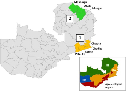
Table 1 Characteristics of study sites, 2008.

	Site 1		Site 2
	Mean	SD	Mean	SD
District population density (persons/km^2)	44.78	(11.96)	12.19	(4.93)
Village distance to main road (km)	13.00	(11.73)	20.37	(20.80)
Household (HH) Size	5.55	(2.73)	5.49	(2.39)
1 = HH head completed primary school	0.25	(0.44)	0.53	(0.50)
1 = HH was poor (below $1 per capita per day)	0.92	(0.27)	0.82	(0.38)
Proportion income derived from off-farm sources	0.22	(0.26)	0.45	(0.42)
Tropical Livestock Units (excluding oxen)	3.10	(5.27)	0.55	(1.62)
Value of equipment/oxen (100s ZMK)	11.36	(21.50)	1.32	(8.11)
Obs.	1044		424
Of cropping households
1 = Smallholder HH (≤5 ha owned)	0.92	(0.27)	0.89	(0.32)
1 = Emergent farmer (5–20 ha owned)	0.06	(0.24)	0.08	(0.27)
Land cultivated (ha)	1.78	(1.43)	1.60	(1.37)
Number of field crops planted	2.66	(1.13)	2.62	(1.14)
1 = HH applied fertilizer	0.38	(0.49)	0.31	(0.46)
1 = HH owned water pump	0.00	(0.07)	0.00	0.00
Obs.	1032		395
No. cropping HHs	194,675		74,310

Source: SS 2008.

3 Methods

3.1 Overview of the farm household models

This paper includes four farm household models that reflect the conditions of (a) a representative smallholder household and (b) a representative emergent farmer household in each of our two study sites. These mathematical programming models for farm-level decision-making incorporate basic household characteristics (e.g., labor and land endowments), budgets for a variety of crop activities, and timelines of crop management. As the objective function is linear, these are linear programming (LP) models. All farm-level decisions on land preparation and crop choice and management are assumed to be made at the beginning of the agricultural season (or in the case of cassava production, the first season). Following Siegel and Alwang (2005), non-crop production activities are assumed to occur outside of the time designated for farm work, with no trade-off between on-farm work and off-farm household and income-generating activities. We further assume that economic factors and government policies are fixed, such that climate is the only variable driver of the production process. While far from realistic, this condition prevents the model from growing too complex and limits the need for assumptions about future price trends. This study intends to capture the impact of climate change only as it is experienced through changes in crop yield.

The household’s objective is assumed to be the maximization of calorie production:(1) $Maxcalories={\sum }_{j=1}^n{K}_j{X}_j$(1) subject to input requirements for each crop activity and the household’s resource constraints:(2) ${\sum }_{j=1}^m{a}_{ij}{X}_j\le b_i$(2) and the non-negativity constraint:(3) $X_j\ge 0$(3) where X_j = hectares (ha) allocated to crop activity j

C_ij = cost of input i used for one ha of production of activity j

a_ij = quantity of resource i required for one ha of production of activity j

b_i = amount of resource i available to the farm-household

K_j = calories produced from one ha of production of activity j

The model assumes that crop production is of the Leontief functional form, such that all inputs can be scaled up proportionally to produce more of a given crop activity, and the model is solved using the simplex LP method.⁴ For one crop, cotton, there is a need to translate yield into ‘calorie content’, and this is accomplished using the site-specific sales price of cotton, coupled with the retail price of maize meal. In other words, we estimate how much maize meal a household could purchase with revenue from cotton production. This is the only crop for which the sales price implicitly enters the objective function.

In the models, a representative farmer is presented with a set of crop activities (also referred to as crop ‘regimes’) to which land will be allocated in order to maximize calorie production. To select these activity options, we first identified the common cropping patterns currently practiced in each site, disaggregated by household type (see Table A1 in Appendix A). These values are derived from a pooled sample across all years for which information on fallow/virgin land was available. After selecting the crops to be included in the models, we next identified the most common regimes, where a crop regime is defined as a combination of crop cultivar and management choices, including seed type (local or hybrid/improved), tillage method (hand or plough), time of land preparation (before or after the start of the rainy season), and fertilizer use (fertilizer applied or not applied). However, because the commonly observed regimes do not necessarily represent a diverse range of management practices, several less common regimes are also included.⁵ The crop regimes for each site are listed in Table 2. In addition, households always retain the option to keep land fallow. This loosely follows the model construction of Siegel and Alwang (2005).

Table 2 Crop activities in farm household models.

	Crop	Seed Type	Tillage Method	Fertilizer	Time of Tillage	Code
Site 1	Maize	Local	Hand	No	Early	MZ1
	Maize	Hybrid	Hand	Yes	Late	MZ4
	Maize	Local	Ox	No	Late	MZ6
	Maize	Local	Hand	Yes	Early	MZ9
	Groundnuts	Local	Hand	No	Early	GR1
	Groundnuts	Local	Hand	No	Late	GR2
	Groundnuts	Local	Ox	No	Late	GR6
	Groundnuts	Improved	Hand	No	Late	GR12
	Sunflower	Local	Hand	No	Late	SUN2
	Sunflower	Improved	Ox	No	Late	SUN10
	Sweet potatoes	Local	Hand	No	Late	SP2
	Sweet potatoes	Improved	Hand	No	Late	SP12
	Cotton	Improved	Ox	No	Late	COT10
	Cotton	Improved	Hand	No	Late	COT12
Site 2	Maize	Local	Hand	No	Early	MZ1
	Maize	Local	Hand	No	Late	MZ2
	Maize	Hybrid	Hand	Yes	Early	MZ3
	Maize	Hybrid	Ox	Yes	Late	MZ4
	Groundnuts	Local	Hand	No	Early	GR1
	Groundnuts	Local	Hand	No	Late	GR2
	Groundnuts	Local	Ox	No	Late	GR6
	Groundnuts	Hybrid	Hand	Yes	Late	GR12
	Cassava	Local	–	–	–	CAS1
	Cassava	Improved	–	–	–	CAS2
	Sweet potatoes	Local	Hand	No	Late	SP2
	Sweet potatoes	Improved	Ox	No	Early	SP12
	Finger millet	Local	Hand	No	Early	MIL1
	Finger millet	Local	Hand	No	Late	MIL2
	Mixed Beans	Local	Hand	No	Early	MB1
	Mixed Beans	Local	Hand	No	Late	MB2
	Rice	Local	Hand	No	Early	RIC1
	Rice	Local	Hand	No	Late	RIC2

Table A1 Crop distributions by area (proportions).

Crop	Site 1		Site 2
	Smallholder	Emergent	Smallholder	Emergent
Maize	0.53	0.40	0.21	0.16
Groundnuts	0.13	0.08	0.07	0.04
Cassava			0.22	0.11
Sunflower	0.06	0.05
Sweet Potatoes	0.00	0.00	0.01	0.01
Finger Millet			0.05	0.03
Mixed Beans			0.12	0.08
Rice			0.05	0.01
Cotton	0.15	0.15
Fallow	0.13	0.32	0.25	0.56
Observations^a	3973	1054	1430	854
Total proportion of accessed land area that is covered by the above crops and fallow	0.97	0.97	0.98	0.99

Sources: SS 2008, CFS 2008–2010.

a ‘Observations’ refers to the total number of households captured in the pooled sample.

For each crop regime, the models include mean yields and the corresponding calories produced (Table 3), as farmers must consider the expected crop yields when allocating land to maximize calorie production. Cases of zero yield, as when a farmer is unable to harvest anything from a field, are dropped for yield estimates (and will also be dropped for the statistical yield models). For cotton and cassava, which are thought to quickly deplete the soil of nutrients (Howeler, 1991; Kidron et al., 2010), we impose an additional requirement that the household leave fallow an area of land equal to that planted to these crops. For example, the model may select 0.5 ha of cotton but must also leave 0.5 ha of land fallow. This captures farmers’ concerns regarding the maintenance of soil fertility, a factor that would not be reflected in the model otherwise.

Table 3 Productivity of crop regimes.

Site 1				Site 2
Crop regime	Obs.^a	Mean yield (kgs/ha)	Calories/ha (1000 s)	Crop regime	Obs.	Mean yield (kgs/ha)	Calories/ha (1000 s)
MZ1	1769	1,104.86	3944.34	MZ1	499	1597.64	5703.57
MZ4	1374	2,322.20	8290.25	MZ2	1074	1491.18	5323.52
MZ6	1456	1,196.34	4270.93	MZ3	495	3249.41	11,600.38
MZ9	1012	1,558.06	5562.26	MZ4	994	3337.59	11,915.21
GR1	710	551.40	3027.17	GR1	596	822.41	4515.02
GR2	2422	483.67	2655.35	GR2	1990	636.05	3491.89
GR6	1670	491.28	2697.10	GR6	136	541.99	2975.52
GR12	1030	454.83	2497.04	GR12	84	556.75	3056.55
SUN2	987	470.05	2284.45	CAS1	529	4776.48	7116.96
SUN10	715	502.38	2441.58	CAS2	232	7173.12	10,687.95
SP2	188	3,385.78	4096.79	SP2	440	3636.86	4400.60
SP12	138	4,591.56	5555.79	SP12	293	4234.55	5123.81
COT10	1237	909.91	6343.09^b	MIL1	711	1008.54	3439.10
COT12	2405	897.94	6259.68	MIL2	901	983.59	3354.04
				MB1	356	604.76	2219.47
				MB2	2298	595.37	2185.01
				RIC1	248	1505.20	5177.90
				RIC2	150	1079.08	3712.04

Sources: Yields: CFS 2008–2010 (cassava), CFS 2003–12 (all other crops); Calories: Wu Leung et al. (1968); Prices: SS 2004 and 2008, RALS 2012.

a When fewer than 30 observations are found within a study site, the geographic range is expanded to the province.

b Cotton harvest is translated into calories through the site-specific median cotton sales price and retail price of maize meal.

Each crop regime is characterized by a timeline of labor requirements that details the biweekly number of worker-days necessary to cultivate one ha. For maize, cassava, and rice, the amount of labor required for different activities (land preparation, planting, fertilizer application, weeding, harvest, and post-harvest activities) is estimated from the CFS (2011 and 2012), while estimates for the remaining crops are taken from a secondary source (Siegel and Alwang, 2005). The timeline of these tasks for a ‘typical year’ was produced in a series of focus group discussions, held in 2011/12 with farmers in each site. Note that these biweekly labor requirements, coupled with the household labor constraints, are instrumental in driving our LP models to arrive at an optimal activity set comprised of diverse crop activities, rather than “specializing”, or allocating all land to a single crop regime. Each crop regime is also characterized by a detailed summary of variable costs, including the costs of fertilizer, seed, and plough rental for land preparation. See ^{Table A2Table A3} in Appendix A for examples of the labor timeline and budgets for select crop regimes.⁶

Table A2 Labor requirements (workdays per ha) for selected crop regimes (site 1).

Month	Half of month	MZ4	MZ6	SUN10	COT10	COT12
October	1
	2				4.50
November	1				5.50	15.00
	2		7.41		1.00	15.00
December	1	5.71	13.05		3.20	1.00
	2	15.00	25.44	8.00	3.20	1.00
January	1	15.24	19.80	10.60	3.20	7.50
	2	13.84	14.80	2.60		7.50
February	1	11.28		11.99	3.20
	2	2.75		11.99	3.20	7.50
March	1	2.75		11.99		7.50
	2	2.75
April	1
	2			6.80
May	1	5.87		9.80
	2	5.87	12.35	3.00	14.15	16.65
June	1	5.87	20.10		15.22	18.25
	2	7.92	7.75		15.22	18.25
July	1	7.92	7.75		1.07	1.60
	2	7.92

Sources: CFS 2011 and 2012 (maize, cassava, and rice), Siegel and Alwang (2005) (other crops), focus groups (timeline of agricultural tasks).

Table A3 Variable costs of crop activities (site 1).

Crop regime	Basal fertilizer (Kg/Ha)	Top fertilizer (Kg/Ha)	Seed/planting material (Kg/Ha)	Basal fertilizer (ZMK/Kg)	Top fertilizer (ZMK/Kg)	Seed/planting material (ZMK/Kg)	Plough (ZMK/Ha)	Total Variable Costs (ZMK/Ha)
MZ1			30.80			0.08		2.43
MZ4	132.07	140.43	25.65	2.46	2.62	6.80		867.69
MZ6			29.77			0.08	40.81	43.16
MZ9	103.69	134.19	29.39	2.46	2.62	0.08		609.34
GR1			51.83			0.32		16.43
GR2			39.87			0.32		12.64
GR6			46.84			0.32	40.81	55.66
GR12			46.09			2.73		125.63
SUN2			14.13			0.58		8.22
SUN10			13.53			8.04	40.81	149.62
SP2			631.08			0.03		17.68
SP12			695.15			0.10		67.67
COT10			26.95			3.91	40.81	146.07
COT12			26.68			3.91		104.19

Sources: SS 2004 and 2008, and RALS 2012 (fertilizer prices); CFS 2012 (seed and plough prices); CFS 2003–2012 (fertilizer/ha); RALS 2012 (seed/ha).

Note: Expenditures on herbicides and pesticides are omitted, as they are used by only a small proportion of Zambian households (4.36% and 12.22%, respectively) (source: RALS 2012).

Note: All figures are mean values, specific to the study site. When fewer than 30 observations are found, the geographic range is expanded to province. Seed that was free or saved from an earlier harvest is included in these estimates as having a cost of zero.

The key strength of a MP model is its ability to capture the trade-offs among a farmer’s options, subject to a set of constraints. Thus, the models are constrained by the average landholding size in each site for specific household types (Table 4). Each model also includes a budget constraint that is loosely estimated with reference to the available information on fertilizer expenditures. The composition of a typical household determines the labor endowment of the representative household. Assuming that each household member between the ages of 15 and 59 is able to contribute 20 workdays per month to farm labor (following Siegel and Alwang 2005), we estimate the household labor available. For example, as a typical smallholder household in site 1 contains 2.65 working-age members, the model is parameterized with a labor endowment of 26.5 workdays per two-week interval. This is the time-step captured in our labor timelines. In addition to family labor, the models also allow for the hiring-in of labor at the local agricultural wage rate,⁷ up to a maximum of five days within each two-week interval.

Table 4 Household endowments and crop productivity (mean values).

	Site 1		Site 2
	Smallholders	Emergent farmers	Smallholders	Emergent farmers
Land owned (ha)	1.92	7.33	1.49	8.46
Prime-age members	2.54	3.16	2.66	2.56
Adult equivalents	4.11	5.05	4.04	4.74
Fertilizer expenditure (ZMK)	267.94	1,105.70	206.80	615.31
Crop calories produced (1,000 s)	6482	21,905	5963	19,826
Gross value crop production (ZMK)	2756	9253	2927	10,736
Observations	1952	400	598	231

Sources: SS 2008 and RALS 2012 (pooled).

3.2 Estimation of the yield effects of climate change

To predict the likely crop choices under an altered climate, the farm household models are to be ‘shocked’ with a new set of expected yields that reflect the extent to which the different crop regimes will likely be affected by climate change. Statistical yield functions are used to capture crop sensitivity to seasonal rainfall and temperature variation, and these are based on field-level data collected in the CFS over nine years for which we have both seed type and weather data (2003–2011). To begin, the yield observations are aggregated from field- to district-level, as such spatial aggregation has been found to produce more reliable results. This is because noise in the explanatory variables induces attenuation bias, whereas aggregation to broader spatial scales cancels out the measurement errors at individual locations (Lobell and Burke, 2010). In this study, measurement errors are found in both the yield estimates of farmers and in climate measures that do not capture microclimatic variations. We apply the model to yield data from all of Zambia rather than construct a time-series model for each site. Though this choice restricts all sites to the same yield-climate relationship, it greatly expands the sample size and exploits the wider variation in both temperature and rainfall found across the country. In a study of statistical yield model validity, this method was also found to be less sensitive to the number of years of data available (Lobell and Burke, 2010).

The linear yield models are of the form:(4) $\ln \left(Meanyiel{d}_{tdcsf}\right)=f\left(yea{r}_t,rai{n}_{dt},rai{n}_{dt}^2,tem{p}_{dt},tem{p}_{dt}^2,CVrai{n}_{dt},\mathrm{districts}\right)$(4) where yield = kgs/ha, t = year, d = district, c = crop, s = seed type (1 = improved), f = fertilizer use (1 = yes), year_t is the number of years from 2003, rain_dt = total rainfall in district d and year t over the November-March growing season, CVrain_dt = the coefficient of variation in monthly rainfall over the five-month growing season in district d and year t, temp_dt = the average temperature over the growing season in district d and year t, and districts = a vector of district dummy variables. We do not build yield functions specific to crop regimes (with consideration of planting time and land preparation method), partly because these factors are assumed to be less important determinants of crop yield (particularly in relation to the seasonal climate variables used in this analysis), and partly because an adequate number of observations could not be found for each specific regime. We follow a common approach of using the logged yields as the dependent variable (Lobell and Burke, 2010), such that the coefficient on a climate variable can be interpreted as a percent change in yield.

Note that not all crops are influenced by the same climate variables in the same functional form. Regressors are therefore selected with a forward stepwise variable selection procedure based on the Akaike Information Criterion (AIC) (Rowhani et al., 2011; Holzkämper et al., 2012), with all season-level variables and district dummies from equation (4(4) $\ln \left(Meanyiel{d}_{tdcsf}\right)=f\left(yea{r}_t,rai{n}_{dt},rai{n}_{dt}^2,tem{p}_{dt},tem{p}_{dt}^2,CVrai{n}_{dt},\mathrm{districts}\right)$(4) ) as candidate regressors.⁸ Goodness-of-fit is based on the AIC in order to minimize the number of climate predictors, as too many variables may lead to over-fitting and a model that is difficult to interpret (Holzkämper et al., 2012;Lobell et al., 2007). For local cassava, with a growing period that extends over two seasons, the model includes both the previous and current years’ seasonal climate outcomes as candidate climate regressors.

Once the yield functions are specified, yield estimates for each site under alternate seasonal climate conditions can be calculated. To capture the baseline climate conditions at each site, we refer to a nearby meteorological station.⁹ Precipitation records cover 50 or 60 years (1960/61 or 1950/51–2009/10), while temperature records cover 31 years (1980/81–2009/10). The average temperature, rainfall, and monthly coefficient of variation of rainfall (CVrain) over the growing season are given in Table 5. For monthly predictions of rainfall and temperature around the year 2050, we refer to the IPCC (2013b) for one relatively ‘wet’ climate model that predicts rainfall increases in Zambia (CCSM) and one relatively ‘dry’ model (HadCM3). Future predictions of each climate variable are converted into a proportion change from baseline with reference to WorldCLIM, which represents climate conditions for the period 1950–2000. This proportion change is then applied to the observed climate averages, based on the meteorological station records, to estimate future climate conditions under each GCM at each site. Estimated yield changes are given in Table 5, with an example of select yield functions given in Table A4 in Appendix A.¹⁰

Table 5 Climate predictions of HadCM3 and CCSM.

		Baseline		Year 2050
		Meteorological station data		Expected% change (GCM projections)
Site	Climate variable^a	Mean	SD	HadCM3	CCSM
1	Rainfall (mm)	989.70	(286.25)	−8.34	3.84
	Average temperature (°C)	24.20	(0.46)	9.76	9.26
	CV rain within season	0.48	(0.16)	1.89	−0.23
2	Rainfall (mm)	1,039.47	(214.82)	−0.75	6.93
	Average temperature (°C)	20.46	(0.66)	10.52	9.43
	CV rain within season	0.37	(0.19)	9.32	3.67

a All variables refer to the November–March growing season.

Table A4 Derivation of expected yield changes for selected crop regimes (site 1).

	Coefficients								Estimated% change
	Year	Rain	Rain^2	Temp	Temp^2	CVrain	Obs.	Adj. R^2	HadCM3	CCSM
MZ4	0.04	1.41E-03	−5.83E-07	−0.02		−0.52	627	0.46	−8.22%	−4.02%
	(0.00)	(0.00)	(0.00)	(0.20)		(0.00)
MZ6	0.02	1.49E-03	−6.62E-07	−0.01		−0.56	642	0.39	−5.48%	−2.24%
	(0.00)	(0.00)	(0.00)	(0.41)		(0.00)
SUN10	0.06			0.02		−0.45	313	0.27	+5.37%	+5.53%
	(0.00)			(0.40)		(0.01)
COT10	0.03	−2.51E-04		2.42	−0.05	−0.82	245	0.36	+5.05%	+3.98%
	(0.01)	(0.05)		(0.00)	(0.01)	(0.00)
COT12	0.03	−2.51E-04		2.42	−0.05	−0.82	245	0.36	+5.05%	+3.98%
	(0.01)	(0.05)		(0.00)	(0.01)	(0.00)

Sources: ZMD and IPCC (2013b).

P-values in parentheses. Coefficients of district dummies selected as regressors are not shown.

Although the estimated yield impacts of climate change differ under the HadCM3 and CCSM predictions, the relative impacts across crops are similar under both scenarios (Table 6). Furthermore, the yield impacts seem to occur mostly through changes in temperature rather than precipitation. Several crops appear to be particularly robust to climate change. Local (traditional) sweet potato is generally unaffected by climate variation, while sunflower, cassava, and cotton seem to benefit from increased temperatures. These results are not particularly surprising, as cassava has been found to be neutral or even to benefit from climate change in sub-Saharan Africa (Blanc, 2012; Jarvis et al., 2012; Liu et al., 2008). Elsewhere in Africa, cotton yields are also predicted to increase with climate change (Butt et al., 2005). Along these lines, Schlenker and Roberts (2009) find that cotton yields increase up to a threshold of 32 °C. Our results indicate that other crops are quite sensitive to climate change in Zambia, including beans, finger millet, and sorghum, and similar results are seen in some (though not all) other studies (Blanc, 2012; Butt et al., 2005; Ramirez-Villegas and Thornton, 2015).¹¹ Our results further suggest that maize yield changes in Zambia will be moderate, declining by 2.24–12.55%. For comparison, Rosenzweig et al. (2014) estimate that maize yields will experience neither significant increases nor decreases in Southern Africa, and Schlenker and Roberts (2009) find that maize yields tend to increase up to a threshold of 29 °C. In our two study sites, the average growing season temperature is 24.20 °C (site 1) and 20.46 °C (site 2), while the average daytime maximum temperature is 29.39 °C (site 1) and 25.24 °C (site 2). Particularly in site 2, this does suggest that there is room for maize yields to improve with rising temperatures before they begin to suffer.

Table 6 Estimated yield changes under climate change scenarios.

Site 1			Site 2
	Expected% change			Expected% change
Crop regime	HadCM3	CCSM	Crop regime	HadCM3	CCSM
MZ1	−5.48	−2.24	MZ1	−4.79	−2.77
MZ4	−8.22	−4.02	MZ2	−4.79	−2.77
MZ6	−5.48	−2.24	MZ3	−6.72	−3.86
MZ9	−12.55	−11.42	MZ4	−6.72	−3.86
GR1	−41.25	−37.05	GR1	+4.00	+5.68
GR2	−41.25	−37.05	GR2	+4.00	+5.68
GR6	−41.25	−37.05	GR6	+4.00	+5.68
GR12	−15.18	−12.06	GR12	−15.10	−11.07
SUN2	+3.98	−2.05	CAS1	+5.61	+8.68
SUN10	+5.37	+5.53	CAS2	+5.82	+6.10
SP2	−0.15	−0.24	SP2	−1.06	−1.40
SP12	−14.03	−13.67	SP12	−11.79	−11.23
COT10	+5.05	+3.98	MIL1	−22.41	−21.74
COT12	+5.05	+3.98	MIL2	−22.41	−21.74
			MB1	−10.32	−7.97
			MB2	−10.32	−7.97
			RIC1	−18.92	−17.72
			RIC2	−18.92	−17.72

Source: Authors’ calculation based on CFS (2003–2011) and the climate predictions of Table 5.

It is important to acknowledge that, while statistical yield models are able to capture poorly understood processes related to climate, such as erosion, pest behavior, and pollination dynamics, they do have several drawbacks. They are necessarily simple and unable to capture interactive effects of multiple climate variables; they require an assumption of stationarity (i.e., that past relationships will hold in the future) when used to predict the yield impacts of climate change; and it is uncertain how well they can project beyond the historical range of observed climate conditions (Lobell and Burke, 2010; Lobell et al., 2007). Statistical yield models based on field data are also susceptible to omitted variable bias if additional climate variables, such as wind speed, influence yields and are also correlated with the climate regressors (Auffhammer and Schlenker, 2014). However, statistical yield models have been found to quantify the effects of changes in climate variables with reasonable accuracy (Holzkämper et al., 2012;Lobell and Burke, 2010),¹² and are able to provide yield estimates across the entire range of field crops that are relevant to farmers in Zambia.

4 Results and discussion

Before predicting the crop choices made under a future climate, we first confirm that the models adequately mirror crop choices that a typical farmer in each site makes in reality. To this end, the models are run with baseline crop yields to select the calorie-maximizing choices for each site and household type (Table 7). We validate the models in several ways: First, results are compared to the actual crop distribution (inclusive of fallow land) for each household type, as observed in the household surveys (see Table A1). The percent of land that is ‘redirected’ away from the actual crop distribution is calculated for each model solution, with smaller values indicating a more realistic model. We also compare results to the average gross value of crop production, as well as calorie production from field crops (excluding cotton) for each household type (see Table 4).¹³ For these tests, a smaller value again indicates a more realistic model. A disaggregated presentation of these validation tests is provided in Table A5, while the key results are found at the bottom of Table 7. These results show that some models produce quite favorable values, notably the smallholder model in site 1 and the emergent farmer model in site 2. Both emergent farmer models correctly predict that a considerable amount of land is left fallow.

Table 7 Baseline results.

	Site 1			Site 2
	Crop regime	Smallholder	Emergent	Crop regime	Smallholder	Emergent
Budget constraint (ZMK)		100	650		100	650
Budget constraint binding?		Yes	Yes		Yes	Yes
Land binding?^a		Yes	No		Yes	No
Land cultivated (ha)		1.82	4.31		1.49	3.52
Labor binding (months)		Dec, Jan, June	Jan, Feb, May, June		Oct–Dec	Oct–Dec, June, July
Net returns per AE per day (ZMK)		1.37	3.20		1.90	4.45
Calories per AE per day		4999.95	10,131.01		5498.42	9084.99
Ha per crop regime	MZ1	1.66	0.14	MZ1	0.35	0.00
	MZ4	0.02	0.00	MZ2	0.34	0.12
	SUN10	0.00	2.13	MZ3	0.04	0.36
	SP2	0.03	0.00	GR1	0.16	0.18
	COT10	0.10	2.03	GR6	0.00	1.33
	Fallow	0.10	3.02	CAS2	0.00	0.29
				SP2	0.00	0.00
				SP12	0.36	0.25
				MIL2	0.00	1.00
				RIC1	0.23	0.00
				Fallow	0.00	4.94
Validation tests
Total% difference in land use		36.08	46.03		65.00	26.97
% deviation (gross value production)		21.83	29.18		0.65	22.29
% deviation (calories produced, excluding cotton)		5.46	73.64		35.97	20.72

Source: Authors’ calculations.

a The land constraint can be binding even when some land is left fallow, as the models require that land be left fallow when cotton or cassava are selected.

Table A5 Validation tests of baseline LP models.

Site 1	Smallholder			Emergent
	Prediction	Selection	% Difference^a	Prediction	Selection	% Difference
Crops (ha)
Maize	1.02	1.68	34.47	2.93	0.14	−38.03
Cotton	0.29	0.10	−9.54	1.10	2.03	12.75
Groundnuts	0.25	0.00	−13.00	0.59	0.00	−8.00
Sweet Potatoes	0.00	0.03	1.61	0.00	0.00	0.00
Sunflower	0.12	0.00	−6.00	0.37	2.13	24.07
Fallow	0.25	0.10	−7.54	2.35	3.02	9.21
Total	1.92	1.92		7.33	7.33
Total% difference in land use			36.08			46.03
Gross value production (ZMK)	2756.26	2154.42	21.83	9253.29	6553.29	29.18
Calories produced, excluding cotton (1,000s)	6481.60	6835.72	5.46	21,905.13	5773.78	73.64
Site 2
Crops (ha)
Maize	0.31	0.74	28.36	1.35	0.48	−10.35
Cassava	0.33	0.00	−22.00	0.93	0.29	−7.61
Millet	0.07	0.00	−5.00	0.25	1.00	8.82
Groundnuts	0.10	0.16	4.01	0.34	1.51	13.89
Mixed beans	0.18	0.00	−12.00	0.68	0.00	−8.00
Sweet Potatoes	0.01	0.36	23.16	0.08	0.25	1.90
Rice	0.07	0.23	10.46	0.08	0.00	−1.00
Fallow	0.37	0.00	−25.00	4.74	4.94	2.35
Total	1.49	1.49		8.46	8.46
Total% difference in land use			65.00			26.97
Gross value production (ZMK)	2926.86	2908.08	0.65	10,736.03	8342.43	22.29
Calories produced, excluding cotton (1,000s)	5962.72	8107.97	35.97	19,825.95	15,717.94	20.72

Sources of predicted values: SS 2008, CFS 2008–2010, and RALS 2012.

a The% difference for a given crop is calculated as [(Prediction (ha) − Model selection (ha))/Total land (ha)]*100. The total% difference in land use, our validation test, is calculated as the sum of absolute values of the% land misplaced in the above rows, divided in half. The latter step is necessary because we would otherwise be double-counting each unit of ‘misallocated' land.

The goal of this paper is to determine the optimal cropping choices under climate change. To do so, we shock the models with a new set of expected yields for each activity (Table 6), with all other parameters and constraints held constant. Calories are again maximized with these new yields. Fig. 2 illustrates the shifts in crop choice made by the representative farm-households under the HadCM3 scenario. Although estimated yields under the HadCM3and CCSM climate scenarios do differ, the cropping choices under each scenario are nearly identical (likely because crop yields respond in a parallel fashion under both scenarios). Thus, a preferred crop under the HadCM3 scenario is also preferred under the wetter CCSM scenario, and only the results for HadCM3 are displayed.

Fig. 2 Cropping choices under HadCM3 climate change scenario.

Source: Authors’ calculations

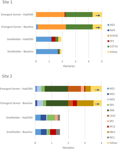
In site 1, there is a shift from maize toward sweet potato and cotton and, for emergent farmers, a slight shift toward sunflower. Specifically, the smallholder allocates 0.47 fewer ha to maize, increases cotton production by 0.12 ha, and expands the area for sweet potato by 0.23 ha. The emergent farmer model has a more moderate response to yields under climate change, although it abandons entirely the production of maize. This pattern is not surprising, as local sweet potato is expected to more resilient than other crops to climate change, and both sunflower and cotton yields are predicted to rise with higher temperatures. (Note that the model does not contain a safety-first constraint that would have restricted the household to produce adequate calories from non-cash crops. With such a constraint, the models would not be able to shift so freely away from maize.) In site 2, the smallholder shifts from rice and sweet potato (both reduced by 0.1 ha) to groundnuts (increased by approximately 0.3 ha), and the emergent farmer now selects an early tillage maize production regime. This accommodates the labor requirements of other crops at the start of the growing season. The emergent farmer also shifts from millet and maize toward improved cassava (with an area increase of approximately 0.5 ha), as cassava yields are expected to improve with higher temperatures. As well, the emergent farmer model allocates slightly more land to groundnuts.

Given these adjustments in cropping choices, farmers are able to reclaim calories that would otherwise be lost if the baseline cropping choices were maintained under climate change scenarios (Table 8). For example, under the HadCM3 scenario, the typical smallholder in site 1 would lose 4.51% of calories produced/acquired if it did not adapt to the new set of expected yields. By allocating more land to cotton production, the farmer is able to recover 1.35% of calories and ultimately loses just 3.16% of calories. In other words, the farmer reclaims 29.98% of the calories that would have been lost without the adjustment of cropping behavior.¹⁴

Table 8 Calories reclaimed or gained through adaptation.

	Site 1		Site 2
	Smallholder	Emergent	Smallholder	Emergent
Baseline
Calories/AE/day	5000	10,131	5498	9085
HadCM3
Calories − Without adaptation	4774	10,619	5071	8548
Calories − With adaptation	4842	10,633	5199	8724
% change in calories with adaptation	−3.16	4.95	−5.44	−3.97
% calories reclaimed/gained through adaptation	1.35	0.14	2.34	1.94
% calories reclaimed through adaptation (of what would be lost)	29.98	N/A	30.03	32.83
CCSM
Calories − Without adaptation	4915	10,559	5158	8690
Calories − With adaptation	4942	10,561	5297	8841
% change in calories with adaptation	−1.17	4.25	−3.67	−2.68
% calories reclaimed/gained through adaptation	0.53	0.03	2.53	1.66
% calories reclaimed through adaptation (of what would be lost)	31.08	N/A	40.81	38.26

Source: Authors’ calculations.

In order to capture the stochastic nature of climate outcomes, we next estimate the probability that a smallholder household falls below a given threshold of calories produced (or in the case of cotton, calories acquired), as a function of variable climate outcomes. Recall that the baseline climate conditions for each site are based on local meteorological station observations for 50–60 years (rainfall) or 31 years (temperature). With this information, we identify the fitted distribution of each climate variable in each site, based on the Kolmogorov-Smirnov goodness-of-fit test. We also construct a rank correlation matrix that captures the correlation among climate variables in each site. As expected, seasonal rainfall and average temperature are negatively correlated, as are rainfall and CV rain, while temperature and CV rain are positively correlated in both sites. The optimal cropping choices of each representative household are then ‘frozen’, both at baseline and under each climate change scenario, and a Monte Carlo simulation is run (with 1000 iterations) in which climate variables enter the yield functions stochastically. For baseline, these climate variables are drawn randomly from the multivariate distributions constructed from the baseline data. For future scenarios, the baseline distributions are shifted to the new expected values while preserving the spread and cross-variable correlations. The spread of each distribution is maintained simply because the GCM predictions do not include an estimate of inter-annual variability.¹⁵

These simulated outcomes are used to estimate the likelihood of falling below two calorie thresholds, including the recommended calorie intake/AE/day (3000) for a medium level of activity (Smith and Subandoro 2007), and the mean level of calories produced/AE/day, as determined by the stochastic model at baseline. Results are given in Table 9. In both sites, it seems that households will continue to meet the 3000 cal threshold with consistency. However, average calorie levels fall under climate change scenarios, with the most severe outcomes occurring under the HadCM3 predictions. This is not surprising, as HadCM3 predicts higher temperatures, lower rainfall, and a higher level of intra-seasonal rainfall variation, which generally result in lower crop yields. Thus, the likelihood that households in site 1 will fail to produce the Monte Carlo baseline mean calorie level (4814 cal/AE/day) increases from 45.6% at baseline to 53.7% under CCSM and 60.2% under HadCM3, even as cropping choices are optimized in each scenario. A similar pattern holds in site 2. These findings demonstrate that households in the future are likely to experience somewhat higher levels of vulnerability than they do today.

Table 9 Smallholder vulnerability to crop shortfalls.

	Mean calories produced or acquired/AE/day	Likelihood of falling below
		3000 cal/AE/day	Monte Carlo baseline mean calories/AE/day
Site 1
Baseline	4813.92	0.80%	45.60%
HadCM3	4606.56	1.20%	60.20%
CCSM	4726.78	0.60%	53.70%
Site 2
Baseline	5309.16	0.20%	41.80%
HadCM3	4934.79	0.70%	70.80%
CCSM	5001.58	0.40%	67.30%

Source: Authors’ calculations.

5 Conclusions and policy implications

This paper has sought to elucidate the likely cropping choices that farmers will make in the future, given crops’ sensitivities to climate change. A mathematical programming approach is used to incorporate the constraints that drive farmer decisions. The models are parameterized with empirical data and calibrated to reflect, as much as possible, the choices that farmers of different types make in present-day Zambia. Results indicate that, when farmers are faced with the estimated yields resulting from an altered climate, they maximize calories by shifting toward sweet potato, cotton, sunflower (Eastern Province), and groundnuts (Northern Province). In doing so, they at least partially offset the losses expected for most crop regimes.

Although the stylized farm household models constructed in this paper are necessarily simple, they provide several key analytical insights on the likely effects of climate change in rural Zambia. First, our statistical analysis indicates that the yield impacts of climate change will differ across crops and management regimes. For example, sweet potato is expected to be relatively unaffected, while cotton and cassava may even benefit from rising temperatures. Farmers are likely to adjust their cropping choices accordingly. As well, these crops may represent ‘low-hanging fruit’ for climate change adaptation, a finding that merits consideration amidst Zambia’s overwhelmingly maize-centric agricultural policies (Jayne et al., 2011). Our results also indicate that maize grown with fertilizer will be somewhat more sensitive than other maize regimes to a warmer climate, thereby reducing the future benefit of fertilizer use. Though fertilizer improves yields, it may not be a solution to the threat of climate change.

Second, the potential for on-farm adaptation to offset the negative effects of climate change should not be overlooked. Farmers in sub-Saharan Africa regularly cope with climate variability by adjusting their management strategies (Twomlow et al., 2008), and it should be expected that they will adapt to climate change in the same manner. Representative smallholder farmers in this paper are able to mitigate the negative yield effects of climate change by recovering or gaining 11.6-38.0% of calories under the HadCM3 predictions (13.0-43.4% under CCSM) that would otherwise be lost without adaptation. However, while the benefits of autonomous adaptation are non-negligible, it seems that in most cases, they are not enough to completely offset the negative effects of climate change. This underscores the importance of larger-scale interventions such as the design of heat-tolerant crop varieties, the development of irrigation infrastructure, and agricultural policies that reduce risk for smallholder farmers. Under a changing climate, farmers will require new and better options within their choice set.

Third, results of this study suggest that smallholder farm-households will still be able to meet their food needs in the future. However, they will experience heightened vulnerability to food shortfalls under climate change, particularly in Northern Province. Furthermore, it is generally expected that climate extremes will become more common in the future (IPCC, 2013a). In other words, the distributions of climate variables will gain ‘fatter tails’, which likely renders our calculation an underestimate of future vulnerability. This anticipated increase in vulnerability may be addressed with policies that promote more diverse agricultural and livelihood portfolios.

Several caveats should be noted: The farm household models are relatively simple in order to prevent the model from growing too complex to allow for clear analytical insights. However, the results should not be interpreted as face-value predictions for what farmers will do, several decades henceforth. This paper does not attempt to capture the other changes that will surely occur in Zambia, including population growth, an increasing commercial orientation of farmers, an increasing mechanization of agriculture, and changes in available infrastructure, such as irrigation. The models do not consider the likelihood of structural transformation characterized by farmers exiting the agricultural sector, nor do we estimate the spread (and/or improved management) of crop and livestock diseases. And we do not account for price feedbacks in an evolving regional and global economy. We are particularly cognizant of another source of environmental change that may affect crops differently, namely soil degradation (Jones et al., 2013). However, an analysis of future crop choice that incorporates a consideration of both climate and soil degradation effects is beyond the scope of the present study. By focusing only on changes in temperature and precipitation, the statistical yield models necessarily do not account for carbon dioxide fertilization, whereby crop yields benefit from rising levels of atmospheric carbon. While we necessarily limit attention to the crops currently grown, new options will undoubtedly be introduced, and cropping patterns may ‘migrate’ with a shifting climate. As well, alternate modelling choices for the yield functions may have produced different estimates of cross-crop sensitivity to climate change.

Despite these limitations, this paper has demonstrated that farmers possess a range of autonomous adaptation options in the form of changes in crop choice and management regimes. These choices merit consideration within the discourse on the likely effects of climate change and the identification of priorities for larger-scale interventions. This paper further highlights the promising role of mathematical programming models, coupled with other analytical techniques, to represent farm-level adaptations to climate change.

Acknowledgments

The authors gratefully acknowledge financial support from the USAID Bureau for Food Security (Associate Award AIDOAA-LA-11-00010 under Food Security III, CDG-A-00-02-00021-00). The Food Security Research Project of Michigan State University provided access to the household data used in this study, and the Zambia Meteorological Department provided access to the historical climate data. The authors also wish to thank Jennifer Olson and Nathan Moore of Michigan State University, as well as Brian P. Mulenga of the Indaba Agricultural Policy Research Institute in Lusaka, Zambia. The views expressed in this study are those of the authors only.

Notes

1 Several abbreviations used in this paper are not standard in the field: AE (adult equivalent); ZMK (Zambian kwacha); and CFS (Crop Forecast Survey).

2 The Ricardian approach assumes that land values are explained partly by climate, and are determined with consideration of all potential future adaptations (Kurukulasuriya and Mendelsohn, 2008; Seo and Mendelsohn, 2008). This method typically measures the net impact of climate change without revealing what adaptations will be made.

3 These three survey rounds refer to the 1999/00, 2002/03, and 2006/07 agricultural years. RALS 2012 refers to the 2010/11 agricultural year, while each CFS refers to the season ending in the survey year.

4 Several variations of the model were considered, including the maximization of profit rather than calories; a nonlinear mean-variance analysis of profit; the inclusion of a safety-first constraint to require the production of a minimum number of calories; and options to rent land at the local market rate. Several of these constructions aim to capture farmers’ attitudes toward risk. Among these variants of the model, we selected calorie maximization as the linear objective function (without any flexibility constraints) in order to best mirror present-day cropping patterns observed in each site, and also to allow the model to adjust freely under new climate conditions.

5 As the models are parameterized with historical data, we are necessarily limited to the crops currently grown in a given site.

6 Due to space constraints, the full labor timelines and crop budgets for both sites are omitted here. However, all values used to construct these models are available from the authors upon request.

7 Wages are estimated with respect to different maize production activities, and differ across the growing season according to the timing of these activities.

8 Where the coefficient on the level temperature term was negative (i.e., the relationship was estimated to be convex), the quadratic term was removed from the list of candidate regressors, thereby imposing a linear relationship between temperature and yield.

9 The meteorological stations selected are Chipata and Mbala stations (sites 1 and 2, respectively).

10 For a given crop regime, the change in yield may differ across sites when the predicted changes in climate variables differ and/or when baseline conditions differ, particularly when temperature and rainfall enter the model in a quadratic manner.

11 In fact, it is somewhat difficult to compare findings across studies that use different methods, GCMs, emissions scenarios, time intervals, and geographic foci (Rosenzweig et al., 2014).

12 Lobell and Burke (2010) conclude that cross-sectional and panel methods are better able to predict yield responses to temperature changes, as compared with precipitation changes. As the HadCM3 and CCSM models both predict greater changes in temperature in Zambia, it seems that statistical models are appropriate.

13 It was at this stage in the model construction process that the objective function was selected, as well as several other features (e.g., the decision to have households rely on their own labor and land holdings without access to a rental market). These model characteristics seem to result in the most realistic baseline model results.

14 For the emergent farmer model in Site 1, which overwhelmingly selects cotton and sunflower at baseline, it seems that calorie production would rise under climate change even without adaptation. In this case, adaptation allows for a further increase in production.

15 Note that, by retaining the same spread of climate variables, we assume the same frequency of weather extremes as found in historical patterns. However, climate change is expected to bring about an increasing frequency of extreme weather, a phenomenon already documented in Zambia (Mulenga et al., 2016).

Appendix A

See ^{Table A1Table A5}.