Use of electromagnetic–terrain conductivity and DC–resistivity profiling techniques for bedrock characterization at the 15th-of-May City extension, Cairo, Egypt

Peer review under responsibility of National Research Institute of Astronomy and Geophysics.

Abstract

A joint multi-spacing electromagnetic–terrain conductivity meter and DC–resistivity horizontal profiling survey was conducted at the anticipated eastern extensional area of the 15th-of-May City, southeastern Cairo, Egypt. The main objective of the survey was to highlight the applicability, efficiency, and reliability of utilizing such non-invasive surface techniques in a field like geologic mapping, and hence to image both the vertical and lateral electrical resistivity structures of the subsurface bedrock. Consequently, a total of reliable 6 multi-spacing electromagnetic–terrain conductivity meter and 7 DC–resistivity horizontal profiles were carried out between August 2016 and February 2017. All data sets were transformed–inverted extensively and consistently in terms of two-dimensional (2D) electrical resistivity smoothed-earth models. They could be used effectively and inexpensively to interpret the area's bedrock geologic sequence using the encountered consecutive electrically resistive and conductive anomalies. Notably, the encountered subsurface electrical resistivity structures, below all surveying profiles, are correlated well with the mapped geological faults in the field. They even could provide a useful understanding of their faulting fashion. Absolute resistivity values were not necessarily diagnostic, but their vertical and lateral variations could provide more diagnostic information about the layer lateral extensions and thicknesses, and hence suggested reliable geo-electric earth models. The study demonstrated that a detailed multi-spacing electromagnetic–terrain conductivity meter and DC–resistivity horizontal profiling survey can help design an optimal geotechnical investigative program, not only for the whole eastern extensional area of the 15th-of-May City, but also for the other new urban communities within the Egyptian desert.

Keywords:

• Multi-spacing electromagnetic–terrain conductivity meter and DC–resistivity horizontal profiling survey
• Bedrock geology
• Eastern extension of 15th-of-May City
• Cairo
• Egypt

1 Introduction

The 15th-of-May City is a distinctive suburban area at the southeastern Greater Cairo established in 1978. The Egyptian New Urban Communities Authority (NUCA) has been targeting to solve the Cairo's insufficient accommodation problem by expanding the surrounding residential areas connected to Cairo. The anticipated eastern extensional area of the 15th-of-May City is roughly centered at latitude 29°49′1.75″N and longitude 31°24′40.20″E, covering an area of some 8.85 km² (Fig. 1). It has an uneven topography, comprising several terraces reaching about 350.0 m above the sea level. Existing relative elevation differences within the area are ranged between 10 and 50 m (Fig. 2b).

Fig. 1 (a) General location and (b) detailed surface geologic maps of the eastern extension of 15th-of-May City, southeastern Cairo, Egypt. The bedrock geology has been constructed based on LANDSAT–TM satellite imagery, aerial photography, surveyed topography and several collected stratigraphic sections using high-resolution global positioning system (GPS) surveying records.

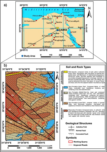
Fig. 2 (a) Recent satellite image (Courtesy: Google Earth^TM Mapping Software–Ver. 7.1.2.2041 Beta, Google Inc., USA) and (b) surveyed topographic contour map of the eastern extension of 15th-of-May City, southeastern Cairo, Egypt. The multi-spacing electromagnetic–terrain conductivity meter and DC–resistivity horizontal surveying profile locations are overlaid.

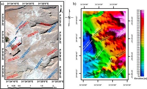
Fig. 7 (a) Measured and calculated weighted-average terrain conductivity responses, using a varying inter-coil spacing above the ground surface at multiple operating frequencies, and (b) 2D transformed–inverted smoothed-resistivity section below the survey profile 2. Warm colors indicate conductive subsurface media, while cold colors indicate resistive subsurface ones.

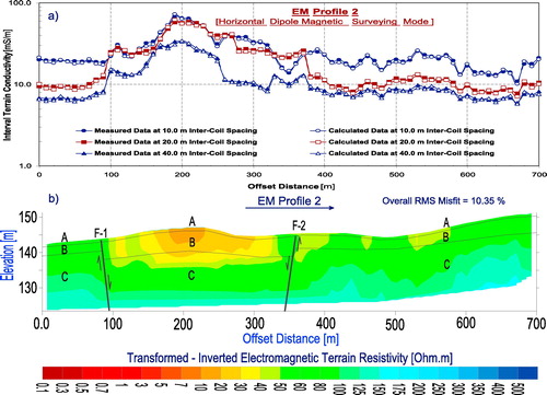
Fig. 8 (a) Measured and calculated weighted-average terrain conductivity responses, using a varying inter-coil spacing above the ground surface at multiple operating frequencies, and (b) 2D transformed–inverted smoothed-resistivity section below the survey profile 3. Warm colors indicate conductive subsurface media, while cold colors indicate resistive subsurface ones.

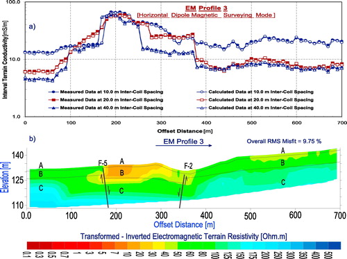
Fig. 10 (a) Measured and calculated weighted-average terrain conductivity responses, using a varying inter-coil spacing above the ground surface at multiple operating frequencies, and (b) 2D transformed–inverted smoothed-resistivity section below the survey profile 5. Warm colors indicate conductive subsurface media, while cold colors indicate resistive subsurface ones.

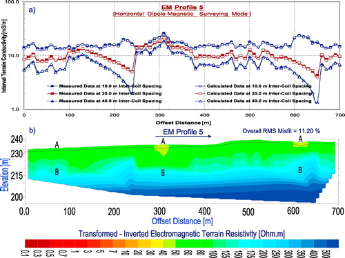
Fig. 14 (a) Measured and (b) calculated weighted-average apparent resistivity pseudo-sections, and (c) 2D inverted smoothed-resistivity section below the survey profile 2. Warm colors indicate conductive subsurface media, while cold colors indicate resistive subsurface ones. (d) The resultant absolute sensitivity section. Large sensitivity values declare high confident inverted resistivities within the section, while small sensitivity values declare low confident ones.

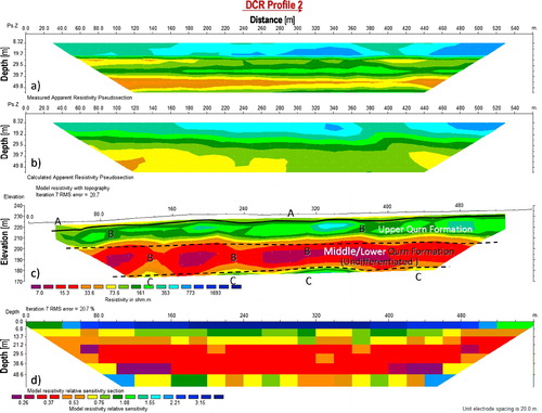
Fig. 15 (a) Measured and (b) calculated weighted-average apparent resistivity pseudo-sections, and (c) 2D inverted smoothed-resistivity section below the survey profile 3. Warm colors indicate conductive subsurface media, while cold colors indicate resistive subsurface ones. (d) The resultant absolute sensitivity section. Large sensitivity values declare high confident inverted resistivities within the section, while small sensitivity values declare low confident ones.

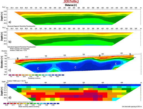
Fig. 17 (a) Measured and (b) calculated weighted-average apparent resistivity pseudo-sections, and (c) 2D inverted smoothed-resistivity section below the survey profile 5. Warm colors indicate conductive subsurface media, while cold colors indicate resistive subsurface ones. (d) The resultant absolute sensitivity section. Large sensitivity values declare high confident inverted resistivities within the section, while small sensitivity values declare low confident ones.

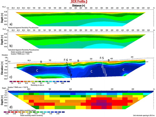
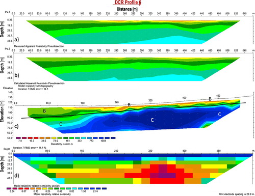
Fig. 18 (a) Measured and (b) calculated weighted-average apparent resistivity pseudo-sections, and (c) 2D inverted smoothed-resistivity section below the survey profile 6. Warm colors indicate conductive subsurface media, while cold colors indicate resistive subsurface ones. (d) The resultant absolute sensitivity section. Large sensitivity values declare high confident inverted resistivities within the section, while small sensitivity values declare low confident ones.

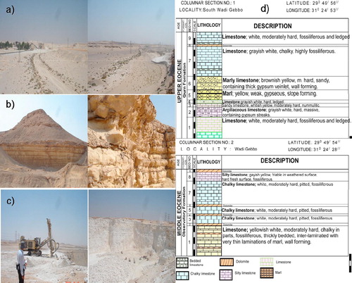
The area's bedrock geology is made up, from the top (recent) to bottom (old) (Figs. 1 and 3), of the followings; (1) the surficial Late Quaternary Wadi deposits, composed mainly of pale yellow/yellowish brown, loose, fine-grained sand and gravel (in granule and pebble sizes) with little/traces of salty/calcareous/gypseous silt and iron oxides. Such thin deposits were developed in very shallow elongated depressions or drainage channels, in the form of small-scale Wadi terraces, fans, and fillings, and could be delivered at the short time spans of annual floods and heavy rains from the adjacent eastern mountainous region; (2) the Upper Eocene Qurn Formation, composed mainly of yellowish white, medium hard, cavernous, Nummulitic, limestone, marl/marly limestone and chalk/chalky limestone with thin dolomite and gypsum bands (Strougo, 1985; Said, 1990). The outcropped thickness is averaged as 65.0 m; and (3) the Middle Eocene Observatory Formation, composed mainly of white/pale yellowish white, fractured, fossiliferous, hard limestone with thin marly limestone and dolomite bands. The outcropped thickness is averaged at 75.0 m, while its total thickness can reach 100.0 m (Mohamed et al., 2012). The area is dissected and transacted by four sets of complex normal faults, trending mainly northwest–southeast. Additionally, its subsurface bedrock is affected by several sets of joints, trending mainly east–west to northwest–southeast (Farag and Ismail, 1959; Moustafa et al., 1985).

Fig. 3 Field photographs showing the encountered area's bedrock geology which is made up of (a) the surficial Late Quaternary Wadi deposits, (b) Upper Eocene Qurn Formation, (c) Middle Eocene Observatory Formation and (d) the typical measured stratigraphic columns within the study area.

Surface electromagnetic induction and electric techniques are nowadays widely used to image the bedrock geologic sequence and its effectual subsurface structures, without disturbing the ground surface, where such a bedrock geology is not accurately known or where ground logistics may restrict the direct drilling (Griffiths and Barker, 1993; Loke and Lane, 2004; Chambers et al., 2006; Sudhaa, et al., 2009; Atya et al., 2010; Gardi et al., 2013; Araffa et al., 2014; Farag, 2015). Consequently, a joint multi-spacing electromagnetic–terrain conductivity meter and DC–resistivity horizontal profiling survey was conducted in the area between August 2016 and February 2017 (Fig. 4). The main objective of the survey was to highlight the applicability, efficiency, and reliability of utilizing such non-invasive surface techniques in a field like geologic mapping, and hence to image both the vertical and lateral electrical resistivity structures of the subsurface bedrock. A total of reliable 6 multi-spacing electromagnetic–terrain conductivity meter and 7 DC–resistivity horizontal surveying profiles were carried out (Figs. 2 and 4).

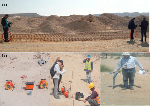
Fig. 4 Field photographs showing the (a) Geonics 'EM–34–3’, (b) ABEM 'Terrameter–SAS–300C' and (c) RadioDetection 'RD–8000’ measuring systems.

2 Multi-spacing electromagnetic–terrain conductivity meter survey

2.1 Conceptual background

Surface electromagnetic induction methods involve the measurement of one (or more) magnetic field components which induced in the subsurface by a primary field produced from a passively occurred or artificially generated source, operating at frequencies less than 1.0 MHz. They have a major advantage over the electric methods is that the induction process doesn't require direct (or galvanic) electrode-contact with the ground. Accordingly, the data can be acquired relatively more quickly and without any logistical difficulties.

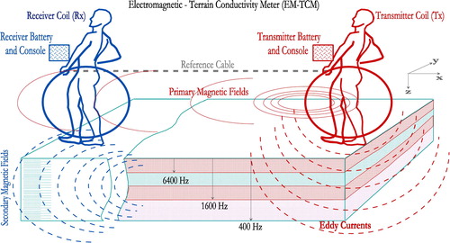
Electromagnetic–terrain conductivity meter techniques are frequency-domain electromagnetic induction methods which use two separate self-contained, multi-turn induction coils connected by a flexible reference cable (McNeill, 1980, 1983); one coil serves as a transmitter to generate the primary magnetic field within the ground and the other acts as a receiver to sense the earth's induced secondary magnetic field, together with the traveled primary field through the air (Fig. 5). They are specifically designed in a way that both coils involve shifting and maintain a fixed separation between them along the survey profile. Where the induction number is much less than unity, then the received the complex quantity 'secondary/primary magnetic fields' is linearly proportional to the subsurface bulk electrical conductivity (McNeill, 1990). Such moving systems measure both the apparent conductivity of the ground in milliSiemens per meter [mS/m] and/or the in-phase component in parts per thousand [ppt] at each measuring point along the survey profile. Typically, there are two modes of operation; horizontal coplanar coils with a vertical magnetic dipole (VMD) and vertical coplanar coils with a horizontal magnetic dipole (HMD). The point of the measurement is usually the mid-coil setting. In VMD orientation the depth-of-penetration is approximately one-and-half the inter-coil spacing, whereas in HMD orientation the depth-of-investigation is approximately one-half to two-thirds the inter-coil separation.

Fig. 5 Field setup of the multi-spacing electromagnetic–terrain conductivity meter measuring system in HMD, using a varying inter-coil spacing above the ground surface at multiple operating frequencies, over a uniform horizontally layered-earth model (modified after Farag, 2015).

The present field measurements were carried out using the commercially available, hand-held 'EM–34–3 system' (Geonics Limited, Canada) (Fig. 4a). The system uses three inter-coil spacings of 10, 20 and 40 m with corresponding three operating frequencies of 6400, 1600 and 400 Hz. Therefore, reliable geometric soundings could be conducted along each survey profile. The data have routinely stacked a minimum of four times at every sounding for data validation and noise evaluation. The system was operated in its HMD mode along each survey profile. Theoretically, the maximum depth-of-investigation is about 35.0 m deep, using the lowest operating frequency of 400 Hz and the corresponding largest inter-coil spacing of 40.0 m. The ambient EM noise levels have been regularly assessed in the field using the metal detector 'RD–8000 locating system' (RadioDetection Limited, UK) (Fig. 4c). Additionally, measurements close to both local sunrise and sunset timing were routinely avoided for not receiving distortions in audio-frequency range (Farag, 2005; AIDUSH Limited, 2006).

2.2 Data processing and interpretation flow

Measured terrain conductivity data sets, along each survey profile, are usually transferred to a PC computer and completely viewed, inspected and transformed via the easy-to-use calculating–plotting program 'EMCalcView−XL−1.0’ (Farag, 2005). Their averages are customarily plotted versus measuring distances (Figs. 6–11). For reconnaissance interpretation, terrain conductivity data viewing and anomaly spotting may suffice. However, the measured interval terrain conductivities at different inter-coil spacings, along each survey profile, in mS/m can be transformed into electrical resistivities in Ohm.m and then plotted against their corresponding normalized resolution depths (levels), i.e., the actual effective skin-depths divided by the inter-coil spacing (Spies, 1989; Farag, 2005; AIDUSH Limited, 2006; Geonics Limited, 2010). They are collectively plotted as a two-dimensional (2D) contoured pseudo-section below the survey profile. This simplest form of semi-quantitative interpretation could introduce a reasonable sequential starting model(s) for the further one-dimensional (1D) smoothed-earth inversion trails stitched in 2D (Figs. 6–11) using the software 'FreqEM^TM–0.1/2006’ (Geotomo Software, Malaysia). The linearized inversion utilized the adaptive-damping scheme in an iterative least-squares optimization fashion (Marquardt, 1963; Keofoed et al., 1972; Inman, 1975; Jupp and Vozoff, 1975; Lines and Treitel, 1984; Guptasarma and Singh, 1997), trying to globally minimize an objective function in which the final 1D solution is regularized. Topographic inputs were implemented within the inversion trials. The final inversion results fit the measured data within 9.75–11.73 RMS %.

Fig. 6 (a) Measured and calculated weighted-average terrain conductivity responses, using a varying inter-coil spacing above the ground surface at multiple operating frequencies, and (b) 2D transformed–inverted smoothed-resistivity section below the survey profile 1. Warm colors indicate conductive subsurface media, while cold colors indicate resistive subsurface ones.

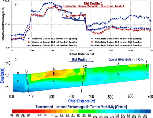
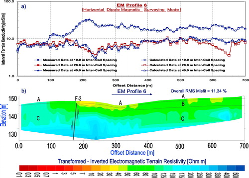
Fig. 11 (a) Measured and calculated weighted-average terrain conductivity responses, using a varying inter-coil spacing above the ground surface at multiple operating frequencies, and (b) 2D transformed–inverted smoothed-resistivity section below the survey profile 6. Warm colors indicate conductive subsurface media, while cold colors indicate resistive subsurface ones.

3 DC–resistivity horizontal profiling survey

3.1 Conceptual background

In typical surface resistivity survey, artificially generated direct current (DC), or very low alternating current (AC) (I) are introduced into the ground using two current-electrodes (C₁, C₂) and the resulting potential differences (ΔV) are measured between them using two potential-electrodes (P₁, P₂). Most commonly used four-electrode configurations are Schlumberger, Wenner, Lee, half-Schlumberger, dipole-dipole, pole-dipole, gradient and square arrays (Parasnis, 1997; Griffiths and King, 1981, Robinson and Courth, 1988; Telford et al., 1990; Keary and Brooks, 1991; Reynolds, 1997; Milsom, 2003). Horizontal electrical profiling survey is usually performed, using popularly the dipole–dipole, pole-dipole or Wenner electrode configurations, with a fixed electrode spacing of a moving array (Fig. 12). This can image the lateral resistivity variation at a depth, reflecting a 2D laterally-contrasted earth model. The depth-of-investigation is highly-controlled by the number-of-stations, current/potential-electrode spacing and number-of-runs along the surveying profile (Roy and Apparao, 1971; Roy, 1972; Apparao, 1997; Oldenburg and Li, 1999). It is also dependent on how much DC–currents can suitably be injected into the ground and the overall signal-to-noise ratio. As a rule of thumb, the maximum separation of current/potential-electrode pairs should be, at least, twice the target depth-of-investigation for an electrical profiling survey. The fundamental transformation equation for calculating ground apparent resistivity is given as ρ_a = K (ΔV/I). The array constant K is known as the 'geometrical factor' (Barker, 1979; Parasnis, 1997) which depends on the relative distances between current and/or potential-electrodes.

Fig. 12 In-line field setup of the multi-spacing dipole-dipole DC–resistivity horizontal profiling survey over a uniform horizontally layered-earth model (redrawn after Loke, 2000).

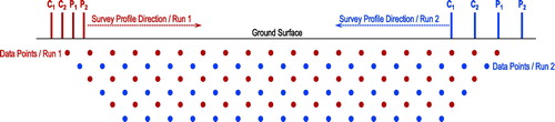
The present field measurements were carried out using the commercially available 'Terrameter–SAS–300C system' (ABEM Instruments AB, Sweden) (Fig. 4b) along 7 surveying profiles. The dipole-dipole configuration was employed with a maximum separation of current/potential-electrode pair of 560 m and 20 m unite-electrode spacing. The apparent resistivity operator can be written as ρ_a = πan (n + 1) (n + 2) (ΔV/I). Where a is the spacing between each current/potential-electrode pairs (dipole length), while n is the number-of-runs (dipole progressive separation) along the whole profiles (Fig. 12). The data have routinely stacked a minimum of four times at every sounding for data validation and noise evaluation.

3.2 Data processing and interpretation flow

Measured apparent resistivity datasets in Ohm.m, along each survey profile, are usually transferred to a PC computer and completely viewed and inspected via the easy-to-use calculating–plotting program 'EMCalcView–XL−1.0’ (Farag, 2005). Their averages are customarily presented in the form of 2D contoured apparent resistivity pseudo-sections for the progressive measurements (Figs. 13–19). They can semi-quantitatively reflect the spatial variation of ground resistivity (Hallof, 1957; Apparao and Sarma, 1981).

Fig. 13 (a) Measured and (b) calculated weighted-average apparent resistivity pseudo-sections, and (c) 2D inverted smoothed-resistivity section below the survey profile 1. Warm colors indicate conductive subsurface media, while cold colors indicate resistive subsurface ones. (d) The resultant absolute sensitivity section. Large sensitivity values declare high confident inverted resistivities within the section, while small sensitivity values declare low confident ones.

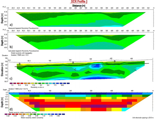
Fig. 19 (a) Measured and (b) calculated weighted-average apparent resistivity pseudo-sections, and (c) 2D inverted smoothed-resistivity section below the survey profile 7. Warm colors indicate conductive subsurface media, while cold colors indicate resistive subsurface ones. (d) The resultant absolute sensitivity section. Large sensitivity values declare high confident inverted resistivities within the section, while small sensitivity values declare low confident ones.

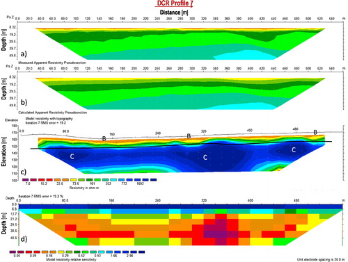
The 2D smoothed-earth inversion of the measured apparent resistivity pseudo-section, below each survey profile, was carried out using the software 'RES2DINV^TM–3.55/2010’ (Geotomo Software, Malaysia) with a standard scheme of successive techniques (Figs. 13–19). No a priori information was initially introduced. The data were inverted using average-apparent-resistivity homogeneous half-space as starting models. Their thicknesses were increased successively in the logarithmic-domain. The linearized inversion utilized the adaptive-damping scheme in an iterative least-squares optimization fashion (deGroot-Hedlin and Constable, 1990; Queralt et al., 1991; Griffiths and Barker, 1993; Loke and Barker, 1995, 1996a, 1996b; Dahlin, 1996; Bernstone and Dahlin, 1997; Dahlin, 2001; Loke and Dahlin, 2002; Zhou and Dahlin, 2003), trying to globally minimize an objective function in which the final 2D solution is regularized. Topographic inputs were implemented within the inversion trials. The final inversion results fit the measured data within 6.50 to 20.70 RMS %. Applying the standard absolute resolution statistics by inspecting the elements of Jacobian or sensitivity matrix for the inverted layer parameters (Jackson, 1972; Sasaki, 1992; Meju, 1994; Dahlin and Loke, 1998; Schwalenberg et al., 2002), typically for the best-fitted resistivity models, was very important as they showed quantitatively how much confidence can be placed in such models (Figs. 13–19).

4 Results and discussion

The final 2D inverted electrical resistivity contoured cross-sections, derived from the interval electromagnetic–terrain conductivities using a varying inter-coil spacing at multiple operating frequencies below the surveying profiles, resulted in a maximum resolution depth-of-investigation of about 35.0 m. The encountered geo-electric sequence (Figs. 6–11) has been shown up with dominant fairly-resistive thin Late Quaternary Wadi deposits [rock type A], constituting mainly of loose, fine-grained sand and gravel (in granule and pebble sizes) with little/traces of salty/calcareous/gypseous silt and iron oxides. The thickness of these surficial deposits is laterally varied, ranging from 0.50 to 1.50 m, from the existing averaged natural ground level. They are partly covering the low/moderately-resistive Upper Eocene Qurn Formation [rock type B], constituting collectively of medium hard, cavernous, Nummulitic, limestone, marl/marly limestone and chalk/chalky limestone with thin dolomite and gypsum bands. Its interpolated thickness can reach 65.0 m. This is followed by the highly-resistive/resistive Middle Eocene Observatory Formation [rock type C], constituting mainly of fractured, fossiliferous, hard limestone with thin marly limestone and dolomite bands. Its complete thickness exceeds the present interpolated maximum depth-of-investigation (about 65.0 m). The sequence is laterally affected by several juxtaposed low/moderately-resistive and highly-resistive/resistive subsurface anomalies. Their lateral contacts can reasonably represent the planes of the geologically known complex normal faults within the area, trending mainly northwest–southeast. Hypothetical schematic drawings, tracing such fault planes, have been suggested and laid over the resistivity cross-sections (F–1, F–2 and F–3).

In agreement, the final 2D inverted electric resistivity contoured cross-sections, derived from the multi-fold apparent resistivities using a varying electrode spacing at multiple DC–horizontal traverses below the surveying profiles, confirmed the obtained geo-electric sequence and lateral structures by electromagnetic–terrain conductivity meter data, and resulted in a maximum resolution depth-of-investigation of about 60.0 m (Figs. 13–19).

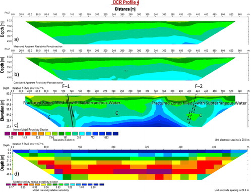
Generally, the above-mentioned geo-electric sequence obviously dips gently to the southwestern direction. Results, along with the field observations, confirmed that the encountered near-surface conductive anomalies below the survey profiles EM–4 and DCR–4 (Figs. 9 and 16, respectively) could be related to the occurred subterraneous water accumulation along the fault planes/traces F–1 and F–2 and suspected fractured zones within the limestone quarry site of Helwan Cement Company.

Fig. 9 (a) Measured and calculated weighted-average terrain conductivity responses, using a varying inter-coil spacing above the ground surface at multiple operating frequencies, and (b) 2D transformed–inverted smoothed-resistivity section below the survey profile 4. Warm colors indicate conductive subsurface media, while cold colors indicate resistive subsurface ones.

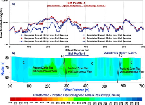
Fig. 16 (a) Measured and (b) calculated weighted-average apparent resistivity pseudo-sections, and (c) 2D inverted smoothed-resistivity section below the survey profile 4. Warm colors indicate conductive subsurface media, while cold colors indicate resistive subsurface ones. (d) The resultant absolute sensitivity section. Large sensitivity values declare high confident inverted resistivities within the section, while small sensitivity values declare low confident ones.

5 Conclusions

The present multi-spacing electromagnetic–terrain conductivity meter and DC–resistivity horizontal profiling field measurements, along with their suggested data treatment and interpretation schemes, demonstrated that their results could be used effectively and inexpensively to image the geo-electric sequence and lateral structures at the anticipated eastern extensional area of the 15th-of-May City, southeastern Cairo, Egypt.

All data sets were transformed–inverted extensively and consistently in terms of 2D electrical resistivity smoothed-earth models. Absolute transformed–inverted electrical resistivity values were not necessarily diagnostic, but their vertical and lateral variations could provide more diagnostic information about the layering and lateral extension of the existing rock types, and hence suggested reliable geo-electric earth models. Nevertheless, such earth models should be used in the context of all a priori information derived from the available drilled boreholes and/or collected stratigraphic sections.

Finally, this study encourages applying the specially-designed multi-spacing electromagnetic–terrain conductivity meter and DC–resistivity horizontal profiling techniques to reliably image both the vertical and horizontal resistivity structures, resulting from the subsurface bedrock geology, with a high-resolution. They can even help design an optimal geotechnical investigative program, not only for the whole eastern extensional area of the 15th-of-May City, but also for the other new urban communities within the Egyptian desert.

Acknowledgment

We are indebted to 'Helal Group for Geotechnical–Geological–Geophysical (3G) Services, Cairo, Egypt' (a private geo-consulting firm operating in Egypt and Arabian countries), for kindly providing RadioDetection 'RD–8000 locating system', during all phases of field measurements, along with the whole topographic surveying data. We would like to thank the editor and reviewers for their constructive comments which helped us to improve the manuscript.

Notes

Peer review under responsibility of National Research Institute of Astronomy and Geophysics.