Sensitivity analysis and mapping the potential groundwater vulnerability zones in Birbhum district, India: A comparative approach between vulnerability models

Peer review under responsibility of National Water Research Center.

Abstract

The assessment of groundwater vulnerability is essential especially in developing areas, where agriculture is the main source of the population. In the present study, four different overlay and index method, namely, DRASTIC, modified DRASTIC, pesticide DRASTIC and modified pesticide DRASTIC are implemented with a view to identifying the most appropriate method that predicts the vulnerable zone to groundwater pollution. Sensitivity analysis reveals that net recharge is the most influential parameter of the vulnerability index. Cross comparison of model output shows the highest similarity of 97% is observed between drastic and modified drastic while the maximum difference in models prediction of 49% is observed between modified drastic and pesticide drastic. Reported nitrate concentrations in groundwater are considered for validation of model-generated final output map. The prediction power of the models are assessed using success and prediction rate method and it highlights DRASTIC model as the most suitable model with 89.69% and 84.54% of the area under area under the curve (AUC) for success and prediction rate respectively.

Keywords:

• Vulnerability index
• Sensitivity analysis
• DRASTIC
• Validation
• Birbhum
• West Bengal

1 Introduction

Intense anthropogenic activities such as the application of chemicals in the agriculture field, industrialization and urbanization put immense pressures on groundwater resource causing degradation of groundwater quality (Oki and Kanae 2006; Kazakis and Voudouris, 2015). A groundwater vulnerability assessment deals with assessing the potential risk of groundwater to both natural and anthropogenic pollutants and their transportation in the aquifer from the surface (Yang et al., 2012). The vulnerability of groundwater is categorized into two types, namely, specific vulnerability and intrinsic vulnerability (National Research Council, 1993). Groundwater vulnerability to a group of contaminants or particular contaminants considering the properties and relationship of contaminants is termed as specific vulnerability (Gogu and Dassargues, 2000). When contaminants are introduced into the ground surface, the ease with which it can reach and diffuse in groundwater is termed as an intrinsic vulnerability. Anthropogenic activities nowadays manipulate the intrinsic vulnerability affecting factors such as soil media, net recharge, depth to groundwater etc. Hence making specific vulnerability more meaningful and important compared to intrinsic vulnerability (Huan et al., 2012).

Various approaches such as such as statistical, process-based, overlay techniques and index methods are applied for mapping the vulnerability of groundwater (Brindha and Elango, 2015). To perform statistical methods (such as principal component analysis, regression analysis, analytical hierarchical process, linear modeling, fuzzy logic models, krigging etc) and process-based approach requires huge reliable data and intensive fieldwork so that meaningful results can be obtained. Whereas, overlay techniques and index methods are simpler approaches to determine the vulnerability of a region based on geological, geomorphological, hydrogeological and other groundwater controlling factors. Various overlay and indexing method such as GOD (Foster, 1987), AVI (Van Stemproot et al. 1993), SEEPAGE (Navulur, 1996), RISKE (Petelet-Giraud et al. 2000), SI (Ribeiro, 2000), DRASTIC (Aller et al., 1987) Modified DRASTIC (Brindha and Elango, 2015) etc. Selection of a particular method to assess the vulnerability of groundwater contamination is very tricky and complicated since the application of different methods may depict significantly different results. Hence, application of multiple models followed by their validation with actual groundwater scenario would be more appropriate rather than deciding the vulnerability of groundwater based on the outputs of the single model.

Mapping of Groundwater vulnerability acts as a basic tool for protection and management of groundwater resources (Margane, 2003; Patrikaki et al., 2012) and is implemented worldwide (Rahman, 2008; Wang et al., 2012). DRASTIC model was implemented for the first time by US Environmental Protection Agency (Aller et al., 1985, 1987), where the name stands for D = Depth to groundwater, R = Recharge rate, A = Aquifer media, S = Soil media, T = Topography, I = Impact of vadose zone, and C = hydraulic Conductivity of the aquifer. Researchers all around the globe have used DRASTIC model for aquifer vulnerability (Huan et al., 2012; Neshat et al., 2014). DRASTIC models and its modified versions typically involve linear combinations of various important factors (Kang et al., 2016). The accuracy of the DRASTIC model has been questioned by many authors and the model has been reported with mixed successes (Rupert 2001; Huan et al., 2012; Kang et al., 2016; Neshat et al., 2014). Numerous studies have been carried out by different researchers with a modification in the DRASTIC models for making it more effective and accurate (Pathak and Hiratsuka, 2010; Wang et al., 2012). Nitrate as an indicator of groundwater pollution for assessment of vulnerability has been used suggested by many researchers (Assafar and Saadeh, 2009; Huan et al., 2012).

Birbhum being one of the important agricultural regions where approximately 81% of land cover is under cultivation sector, the agricultural field is often treated and burden with a huge amount of fertilizers and pesticides which can degrade the groundwater quality through contamination. Several studies on groundwater have been carried out earlier (Mondal et al., 2014; Thapa et al., 2017a,b). Assessment of groundwater vulnerability to pollution has not been carried out in the study area. With this viewpoint, groundwater vulnerability assessment was carried out implementing four different overlay and index methods for vulnerability assessment, namely DRASTIC, modified DRASTIC, pesticide DRASTIC and modified pesticide DRASTIC followed by identifying the most reliable method among them. The model’s accuracy and feasibility are validated with reported nitrate concentration in groundwater as the sources of nitrate in groundwater are mostly anthropogenic rather than geogenic origin.

2 Study area

Birbhum district, also known as the ‘Land of Red Soil’, lies within 23° 32′ 30″ and 24° 35′ 0″ North latitude and 88° 1′ 40″ and 87° 5′ 25″ East longitude and encompasses an area of 4545 sq.km. Location map of the study area is represented in Fig. 1.

Fig. 1 Location map of the study area.

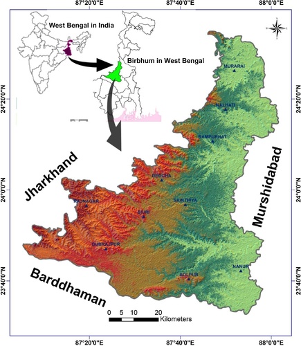
Archean rocks such as biotite-schist, calc-granulites, granites and granite-gneiss are exposed on the surface in the south-western and north-western part whereas basaltic Rajmahal traps are exposed in the northern part of Birbhum district. Tertiary formations show the presence of patchy occurrence. Yellowish-brown older alluvium occurs in the south-eastern and eastern regions. Recent floodplain deposits consisting mainly sand, silt and clay occur along stream course (Mondal et al., 2014; Thapa et al., 2017c).

Groundwater is the principal source of water for drinking and irrigation purpose in the district. The movement of groundwater is towards east from west. Tube wells in the eastern part of the district (average 100 m) are deeper and have higher yield in comparison to western regions of the district. Groundwater in Birbhum occurs in both confined and water-table condition where water table conditions are observed in alluvium, as well as hard weathered rocks and confined conditions, are observed in deeper alluvium. In the Tertiary formation beyond the depth of 136 mbgl (meters below ground level), auto-flow conditions of aquifer occur and the variation in piezometric head varies from 3 to 4 mbgl on an average.

3 Materials and method

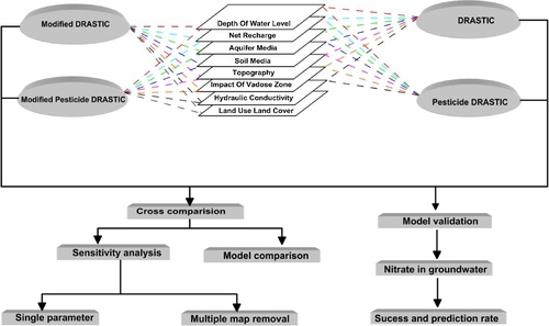
The base map of Birbhum district was demarcated from Survey of India toposheet in 1:50,000 scale. Various input factors viz. depth to groundwater, recharge rate, aquifer media, soil media, topography, the impact of the vadose zone, and hydraulic conductivity of the aquifer were used to carry out the study. Geological Survey of India (GSI) resource map series was used to digitize geomorphology map of the study area. Depth to groundwater, aquifer media and hydraulic conductivity details was gathered from official website of Birbhum district and West Bengal PHED official website (Govt. of West Bengal, 2017; WBPhed, 2017) and net recharge map were generated from annual recharge data collected from Central Groundwater Board (CGWB). Impacts of the vadose zone, land use land cover, rainfall were georeferenced and digitized from district planning map series of NATMO, 2004. Soil texture map was collected from the official website of Birbhum District (http://birbhum.gov.in). These maps are generated with the help of ArcGIS10.1 software. The methodology adopted for the present study is represented schematically in Fig. 2.

Fig. 2 Flow chart of methodology adopted.

3.1 Models for mapping vulnerability

Vulnerability assessment using the index and weighted overlay methods involves selection of factors affecting groundwater vulnerability, followed by their interpretation with assigning weights and rating, computation and demarcation of vulnerability classes. In the models applied, a score of 0–5 is assigned as weights where 0 indicate low pollution potential and 5 indicates relatively high pollution potential. The sub-classes of each input parameters are assigned a rating of 0–10, with 0 meaning low pollution potential and 10 meaning high pollution potential. The weights are multiplied by ranks for generating inputs maps which are overlaid over one another for generating final maps. The details of weights and rating assigned are represented in Tables 1 and 2.

Table 1 Different weights used for different parameters.

Parameter	Depth to water (D)	Net recharge (R)	Aquifer media (A)	Soil media (S)	Topography (T)	Impact of vadose zone(I)	Hydraulic conductivity (C)	Landuse/land cover (LU)
DRASTIC (Aller et al., 1987)	5	4	3	2	1	5	3	Not considered
Pesticide DRASTIC (Aller et al., 1987)	5	4	3	5	3	4	2	Not considered
Modified DRASTIC (Brindha and Elango, 2015)	5	4	3	2	1	5	3	5
Modified pesticide DRASTIC (Brindha and Elango, 2015)	5	4	3	5	3	4	2	5

Table 2 Different rating of each parameter.

Thematic layer	Subclasses	Assigned rating
Depth to water level (m)	0–15	9
	15–30	7
	30–50	5
	50–75	3
	75–100	2
	100 above	1
Net recharge (inches)	0–4	9
	4–7	8
	7–10	3
	10+	6
Aquifer media	Recent alluvium	8
	Basalt with intericapptan clay	9
	Old alluvium with laterite etc.	8
	Gneisses	3
	Older alluvium	8
Soil media	Clay loam	3
	Loam	5
	Clay	1
	Sandy	9
	Sandy loam	6
	Sandy clay loam	5
Topography (percent slope)	Low	1
	Moderate	5
	High	10
Impact of vadose zone	Ferrogeneous sand with clay	6
	Alluvium	8
	Clay with lateritic nodules	3
Hydraulic conductivity (gpd/ft^2)	700–1000	6
	1–100	1
	300–700	4
	100–300	2
	1000–2000	8
	2000 and above	10
LULC (L)	Rural settlements	7
	Urban settlement	7
	Uncultivable land	8
	Wasteland	8
	Water bodies	5
	Forest	0
	Cultivated land	7

DRASTIC index as proposed by Aller et al. (1987) is expressed as follows (Eq. (1(1) $\text{DRASTIC}\text{index}\text{(DI)}=\text{(Dr}\times \text{Dw)}+\text{(Rr}\times \text{Rw)}+\text{(Ar}\times \text{Aw)}+\text{(Sr}\times \text{Sw)}+\text{(Tr}\times \text{Tw)}+\text{(Ir}\times \text{Iw)}+\text{(Cr}\times \text{Cw)}$(1) )): (1) $\text{DRASTIC}\text{index}\text{(DI)}=\text{(Dr}\times \text{Dw)}+\text{(Rr}\times \text{Rw)}+\text{(Ar}\times \text{Aw)}+\text{(Sr}\times \text{Sw)}+\text{(Tr}\times \text{Tw)}+\text{(Ir}\times \text{Iw)}+\text{(Cr}\times \text{Cw)}$(1)

where r represents rating, w represents weight, and D, R, A, S, T, I, C represent the input parameters as described above.

Pesticide DRASTIC index is also calculated using the (Eq. (1(1) $\text{DRASTIC}\text{index}\text{(DI)}=\text{(Dr}\times \text{Dw)}+\text{(Rr}\times \text{Rw)}+\text{(Ar}\times \text{Aw)}+\text{(Sr}\times \text{Sw)}+\text{(Tr}\times \text{Tw)}+\text{(Ir}\times \text{Iw)}+\text{(Cr}\times \text{Cw)}$(1) )) but the weights assigned to input parameters by Aller et al. (1987) are different to DRASTIC index i.e., the weights of D, R, and A input parameters are same whereas the weights of S, T, I and C parameters are different for both DRASIC and pesticide DRASTIC.

In the study area, anthropogenic activities involving the implementation of fertilizer and pesticide in agricultural field acts as prevalent contaminants to groundwater contamination. Hence, the ‘DRASTIC’ model was modified into ‘modified DRASTIC’ model with the incorporation of land use land cover as additional input parameters. Several researchers have implemented modified DRASTIC in their study (Brindha and Elango, 2015). Modified DRASTIC is expressed by the equation below (Eq. (2(2) $\text{Modified}\text{DRASTIC}\text{index}\text{(MDI)}=\text{(Dr}\times \text{Dw)}+\text{(Rr}\times \text{Rw)}+\text{(Ar}\times \text{Aw)}+\text{(Sr}\times \text{Sw)}+\text{(Tr}\times \text{Tw)}+\text{(Ir}\times \text{Iw)}+\text{(Cr}\times \text{Cw)}+\text{(LUr}\times \text{LUw)}$(2) )): (2) $\text{Modified}\text{DRASTIC}\text{index}\text{(MDI)}=\text{(Dr}\times \text{Dw)}+\text{(Rr}\times \text{Rw)}+\text{(Ar}\times \text{Aw)}+\text{(Sr}\times \text{Sw)}+\text{(Tr}\times \text{Tw)}+\text{(Ir}\times \text{Iw)}+\text{(Cr}\times \text{Cw)}+\text{(LUr}\times \text{LUw)}$(2)

where r represents rating, w represents weight, LU is the Land use land cover and D, R, A, S, T, I, C represent the input parameters.

Eq. (2(2) $\text{Modified}\text{DRASTIC}\text{index}\text{(MDI)}=\text{(Dr}\times \text{Dw)}+\text{(Rr}\times \text{Rw)}+\text{(Ar}\times \text{Aw)}+\text{(Sr}\times \text{Sw)}+\text{(Tr}\times \text{Tw)}+\text{(Ir}\times \text{Iw)}+\text{(Cr}\times \text{Cw)}+\text{(LUr}\times \text{LUw)}$(2) ) is also used for calculation of modified pesticide DRASTIC index with weights assigned by Brindha and Elango (2015) The weights of D, R, A and LU input parameters are same whereas the weights of S, T, I and C parameters are different for both modified DRASIC and modified pesticide DRASTIC.

3.2 Sensitivity analysis

Sensitivity analysis (SA) measures the uncertainty or variation in the output results obtained from models applied (Saltelli et al., 2008). In more general term it measures the robustness associated with the model output with manipulated input variables. It helps to understand the influence of individual input parameters on the model’s output by estimating the change in output map with each change in inputs. Researchers have studied the impact of input parameters on the model output which is influenced by several factors such as a number of input parameters, inaccuracy related to inputs, weights, and ranks assigned, nature of overlay performed (Heuvelink et al., 1989). In the present study, two different methods of sensitivity were implemented i.e., single parameter sensitivity analysis (Napolitano and Fabbri, 1996) and Map removal sensitivity analysis (Lodwick et al., 1990) to test the sensitivity of the various hydrogeological parameters. The statistical summary of rating of each parameter used in the study are obtained from in ArcGIS 10.1 software using symbology and classification statistics options of layer properties and the results are represented in Table 3.

Table 3 Statistical summary of rating.

Parameters	Minimum	Maximum	Mean	Standard deviation
D	1	9	4.81	1.99
R	3	9	7.58	1.96
A	3	9	7.14	1.89
S	1	9	4.08	2.44
T	1	10	2.17	1.02
I	3	8	5.1	2.16
C	1	10	2.61	1.76
L	0	8	6.71	1.33

3.2.1 Single parameter sensitivity analysis

Single parameter sensitivity analysis (Napolitano and Fabbri, 1996) is used to assess the influence of individual input parameters on the vulnerability index. The mathematical expression is as follows (Eq. (3(3) $\text{Sp}=\frac{(\text{Rp}\times \mathrm{R}\mathrm{w})}{A}\times 100$(3) )): (3) $\text{Sp}=\frac{(\text{Rp}\times \mathrm{R}\mathrm{w})}{A}\times 100$(3)

where Sp is the sensitivity analysis, ‘Rp’ and ‘Rw’ are the rating and weights assigned to each parameter, and A is the overall vulnerability index of the model used (Table 4). Details of ‘Rp’ and ‘Rw’ assigned to each parameter are represented in Tables 1 and 2 respectively.

Table 4 Single parameter sensitivity analysis.

Parameters removed	Variation index (%)
	Minimum	Maximum	Mean	Standard deviation
DRASTIC
D	0.5	2.7	2	0.7
R	0.5	3.9	3.4	0.3
A	0.7	3	2.2	0.4
S	0.1	2	0.7	0.4
T	0.3	1.3	0.8	0.1
I	0.1	2	0.8	0.8
C	0.2	2.5	0.7	0.5
Pesticide DRASTIC
D	0.3	0.8	1.9	0.7
R	0	3.2	2.7	0.1
A	0.6	2.8	2.1	0.4
S	0.2	5.7	1.6	0.9
T	1	4	1.7	0.3
I	0.7	3	2.2	0.6
C	0.1	1.5	0.4	0.3
Modified DRASTIC
D	0.3	3.2	1.6	0.5
R	0.3	2.4	3.1	0.2
A	0.6	2.5	2.4	0.3
S	0.1	2.4	0.5	0.3
T	0.2	1.3	0.6	0.1
I	0.8	4	1.7	0.6
C	0.1	2	0.5	0.4
LU	0	3.5	1.1	0.5
Modified pesticide DRASTIC
D	0.2	2.8	1.4	0.5
R	0.3	2.1	2.9	0.2
A	0.4	2.1	2.2	0.3
S	0.2	5.3	1.1	0.7
T	0.7	3.4	1.6	0.2
I	0.5	2.8	1.9	0.4
C	0	1.2	0.3	0.2
LU	0	3.2	1.9	0.4

3.2.2 Map removal sensitivity analysis

Lodwick et al. (1990) proposed the measurement of the sensitivity of input parameters with map removal sensitivity analysis where one or more inputs map are removed at a time from a suitability analysis. That method was preferred because it tests the sensitivity of operations between map layers. The equation is computed as follows (Eq. (4(4) $\text{SA}=\frac{|\frac{A}{X}-\frac{B}{Y}|}{A}\times 100$(4) )): (4) $\text{SA}=\frac{|\frac{A}{X}-\frac{B}{Y}|}{A}\times 100$(4)

‘SA’ represents the sensitivity index, ‘A’ and ‘B’ represents the vulnerability indices of unperturbed and perturbed outputs respectively and ‘X’ and ‘Y’ are the number of layers implemented for computing ‘A’ and ‘B’ respectively (Table 5).

Table 5 Multiple map removal sensitivity analysis.

Parameters removed	Variation index (%)
	Minimum	Maximum	Mean	Standard deviation
DRASTIC
DRASIC	0	6.9	1.2	0.6
DRASI	0	6.4	1.6	0.9
DRAI	0	6.7	1.8	1.2
RAI	0.5	10.7	2	1.5
RA	2.1	18.5	4.5	2.8
R	4	28.8	8.3	5.8
Pesticide DRASTIC
DRASIC	0	1.86	1.08	0.7
DRASI	0	3.58	1.43	1.22
DRAI	0	1.04	0.173	0.165
RAI	0.04	7.25	5.62	2.04
RA	0.05	9.58	3.1	2.21
R	1.5	24.14	7.67	4.94
Modified DRASTIC
DRASICL	0	8.13	0.96	0.78
DRASIL	0	7.11	1.22	0.97
DRAIL	0	9.86	1.01	0.75
RAIL	0	11.51	2	1.33
RAL	0	12.48	3.06	1.77
RA	0.03	16.2	7.49	2.67
R	0.02	19.79	5.83	3.78
Modified pesticide DRASTIC
DRASICL	0	7.28	0.7	0.43
DRASIL	0	7.48	0.74	0.57
DRAIL	0	8.51	1.04	0.96
RAIL	0	10.4	1.22	1.06
RAL	0	9.78	1.49	1.36
RA	0	13.08	4.99	2.48
R	0	16.27	4.66	2.87

The unperturbed vulnerability index is obtained by computing all the inputs parameters considered in the study whereas perturbed vulnerability index is the result of removing one or more parameters at a time.

3.2.3 Model comparison

For comparison of maps, the final output maps derived from the different model are reclassified and assigned numbers ranging from 1 to 4 where, 1 represents the low zone, 2 and 3 representing the moderate and high zone respectively and 4 being the very high zone. The reclassified maps of final output maps from the four models used are subtracted with one other and the results are represented in table format where zero values implies that there is no difference in prediction by two models, −1 and 1 indicates a difference of one vulnerability category between the two models, −2 and 2 represent difference of two venerability zones between the model and 3 and −3 implies the difference of three predicted zones.

4 Results and discussion

4.1 Input parameters

4.1.1 D — depth to groundwater

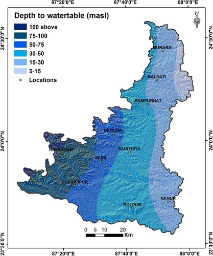
Fig. 3 shows that approximately 97.35 sq.km (2%) of the study area bears groundwater above 100 mbgl (meter below ground level), 1191.73 sq.km (25%) area falls between 60 to 100 mbgl, 2976.25 sq.km (64%) have groundwater between 20 to 60 mbgl and 356.49 sq.km (7.7%) of the total area have groundwater with 20 mbgl. The groundwater tables give detail information about the depth and fluctuation of water over time. Groundwater depth is a crucial data for understanding groundwater, resource quantification, groundwater flow, and depends upon several other factors such as geological and hydrogeological condition, aquifer media, groundwater recharge scenario, precipitation, discharge rates etc. The high vulnerability is associated with low groundwater depth and vice versa.

Fig. 3 Depth to watertable in the study area.

4.1.2 R — net recharge

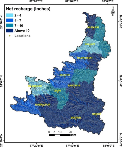
In the study area, approximately half of the area under investigation i.e., 2394.33 sq.km (51.8%) falls have net recharge potential of fewer than 4 in., 825.26 sq.km (17.86%) area has net recharge potential between 4 to 7 in., whereas 502.45 sq.km (10.87%) and 899.80 sq.km (19.47%) area has net recharge potential of 7–10 in. and above 10 in. respectively (Fig. 4). Net recharge refers to the amount of water entering an aquifer. The amount of recharge can be calculated on monthly or annual basis based on data available. Recharge is the main route for transportation of contaminants even though recharging of groundwater dilutes the concentration of contaminants entering into the aquifer. In our study area recharging occurs both naturally and through anthropogenic activities such as check dams, hydropower dam and man-made canal system routing the reclaimed or rainwater to the subsurface.

Fig. 4 Net recharge in the study area.

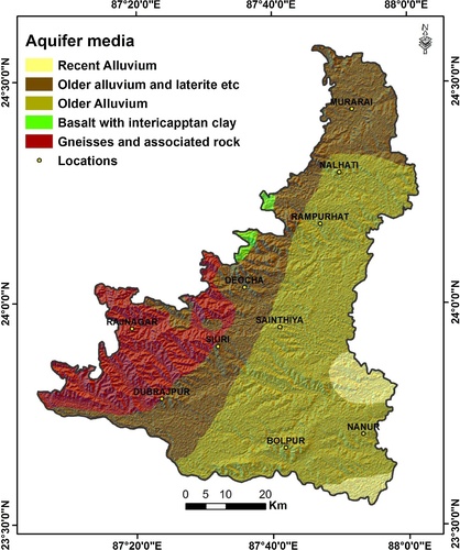
4.1.3 A — aquifer media

Older alluvium aquifers with moderate yield prospect cover approximately half of the study area i.e., 2235.55 sq.km (48%), older alluvium with laterite having limited yield prospect accounts for 29% of total study area i.e., an area of about 1341.66 sq.km, recent alluvium covers an area of 210 sq.km (4.54%), basalt with intericapptan clay accounts for 35.72 sq.km (0.77%) and granite and gneiss account for 17.28% of the study area which encompasses an area of 798.88 sq.km. (Fig. 5). Aquifer media is one of the most important factors influencing the chemical composition of groundwater. Transportation of underground pollutants is highly influenced by the aquifer media. Aquifer associated with higher permeability allows a high amount of water to pass through hence more contaminants reaches the underground water reservoirs.

Fig. 5 Aquifer media in the study area.

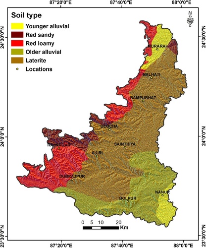
4.1.4 S — soil media

Laterite soil type (Ultisols), younger alluvial (Entisols), older alluvial (Alfisols), red sandy (Alfisols), red loamy (Alfisols) covers approximately 2236.94 sq.km (48%), 318.17 sq.km (6.8%), 976.64 sq.km (20%), 260.99 sq.km (5.65%), and 829.08 sq.km (17.93) respectively (Fig. 6). Soil type of an area has a direct influence on the movement of water and contaminants to the aquifer through leaching from the soil surface. The amount of water percolation is significantly regulated by the soil type (El-Baz et al., 1995). Sorption phenomena and micro-organism in soils promote degradation of contamination to some extent.

Fig. 6 Soil type in the study area.

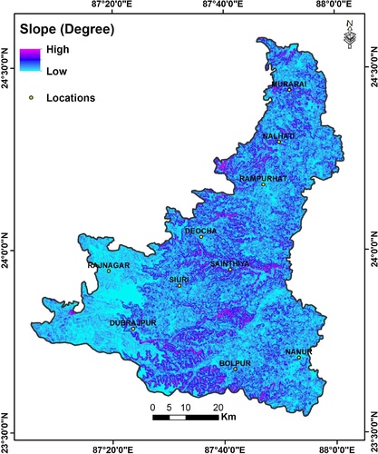
4.1.5 T — topography

The entire study area is classified into three areas on the basis of slope angle i.e., slope <10° covering 3653.51 sq.km (79%), slope 10°–20° and slope 20°–80° covering 932.32 sq.km (20%) and 35.99 sq.km (01%) respectively in the study area (Fig. 7). From elevation point of view approximately 55% areas fall under 50 m elevation, 37% area lies within 50–100 m and 8% area falls above 100 m elevation. The gentle slope is associated with percolation of rainwater and surface runoff to the aquifer. Areas having gentle slope are plainer in topography with reduced drainage velocity. Slope determines whether the groundwater carrying contaminants will reach the groundwater reserve or will flow downhill as run-off. In areas with a steeper slope, the rainwater or surface runoff flows away very quickly giving less time for percolation (Magesh et al., 2011; Waikar and Nilawar, 2014).

Fig. 7 Topography in the study area.

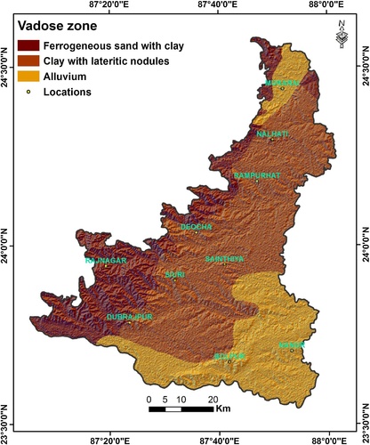
4.1.6 I — impact of vadose zone

In the study area, ferruginous sand with clay, alluvium, and clay with lateritic nodules encompasses an area of 1090.07 sq.km (23.59%), 1294.82 sq.km (28.02%) and 2236.81 sq.km (48.40%) respectively (Fig. 8). Vadose zone is a complex medium for transport of groundwater where the flow rate can vary significantly. The discontinuously saturated or unsaturated soil horizon both above and below the water table is the vadose zone. Vadose zone facilitates the filtration out of harmful chemical through the soil matrix from recharging water entering into the aquifer.

Fig. 8 Impact of vadose zone in the study area.

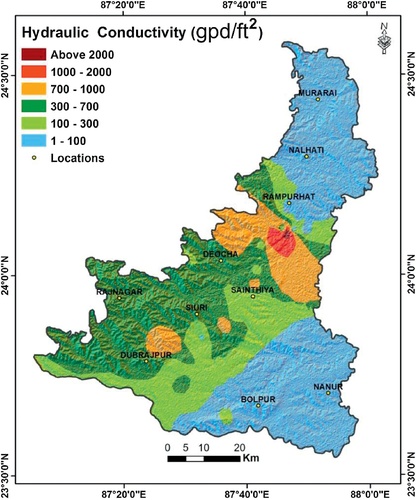
4.1.7 C — hydraulic conductivity

In the study area, hydraulic conductivity is divided into six classes i.e., 1–100, 100–300, 300–700, 700–1000, 1000–2000, and above 2000 (gpd/ft²) encompassing an area of 1932.28 sq.km (41.80%), 842.07 sq.km (18.22%), 1370.43 sq.km (29.65%), 430.80 sq.km (9.32%), 42.76 sq.km (0.93%) and 4.07 sq.km (0.09%) respectively (Fig. 9). Hydraulic conductivity of an aquifer varies significantly due to the heterogeneity of geologic condition and its estimation helps in quantitative prediction of response of the aquifer to recharging and pumping activities.

Fig. 9 Hydraulic conductivity of the study area.

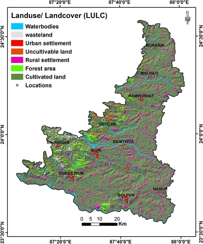
4.1.8 LU — land use/land cover

A major portion of the study area is covered by cultivated area i.e., about 3763.97 sq.km (about 81%), forest area accounts for approximately 3.64% (168.39 sq.km) of the study area whereas rural settlements, urban settlements, industrial land, wasteland, water bodies occupying area of 466 sq.km (10%), 43 sq.km (1%), 46 sq.km (1%), 42 sq.km (1%), 113 sq.km (2%) respectively (Fig. 10). A various hydrological process such as evaporation, infiltration rates, surface runoffs etc is greatly influenced by the type of land cover (Waikar and Nilawar, 2014). The introduction of fertilizers and pesticides in the agricultural field can trigger groundwater contamination.

Fig. 10 Land use land cover map of the study area.

4.2 Models output and cross comparison of models

Cross comparison of models assists to resolve the extent of similarity and dissimilarity of predictions of one model as compared to others models. It is better to implements several techniques for generating different outputs and perform a comparative study before selecting any one method as best and implementing it on a broader area to solve any problem under study. The statistical variation of each input parameter, represented in Table 3, indicates that net recharge contributes most significantly to aquifer vulnerability followed by aquifer media and land use land cover derived from equation (Eq. (3(3) $\text{Sp}=\frac{(\text{Rp}\times \mathrm{R}\mathrm{w})}{A}\times 100$(3) )) (Brindha and Elango, 2015).

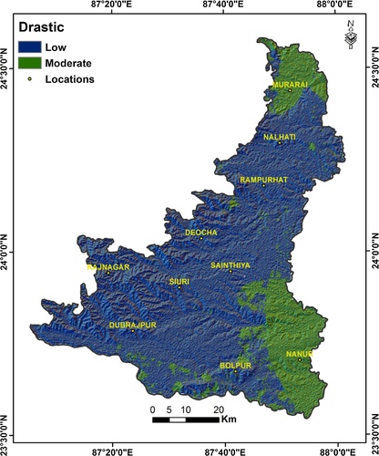
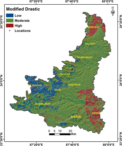
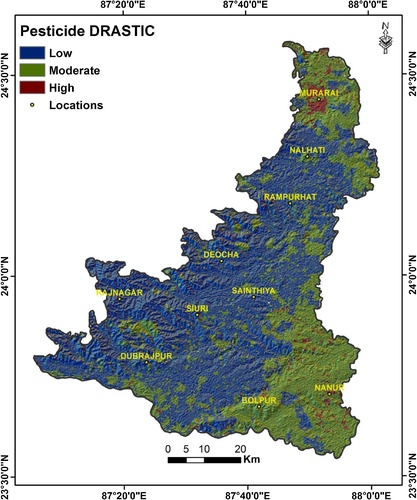
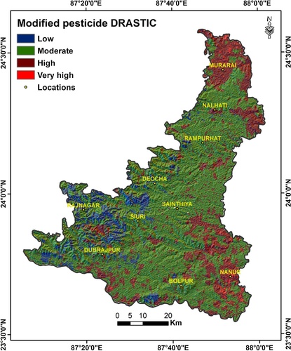
The vulnerability index in DRASTIC model ranges from 65 to 149 and the final output demarcates 3628.91 sq.km (79.88%) and 913.98 sq.km (20.12%) area under low and moderate groundwater vulnerability zones respectively (Fig. 11). In modified DRASTIC, the vulnerability index varies from 65 to 184 and the final output is divided into 3 vulnerability zones viz low, moderate and high encompassing an area of 537.99 sq.km (11.84%), 3486.08 sq.km (76.74%), 518.39 sq.km (11.81%) respectively (Fig. 12). In pesticide DRASTIC, vulnerability indices range from 60 to 187 and the final output of the model illustrates three vulnerability zones i.e., low accounting for 62.77% (2851.10 sq.km) of the total area, medium zone accounting for 35.29% (1602.73 sq.km) and high vulnerability zone covering an area of 1.95% (88.39 sq.km) (Fig. 13). The indices of vulnerability index ranges from 60 to 222 in modified pesticide DRASTIC (Fig. 14) where, low, moderate, high and very high regions covers an area of 357.80 sq.km (7.88%), 3126.01 sq.km (68.85%), 1014.15 sq.km (22.34%) and 42.44 sq.km (0.93%) respectively. Modified pesticide DRASTIC is the only model showing zones having a very high vulnerability to groundwater pollution which attribute to use of land use land cover in this model.

Fig. 11 Vulnerability zonation using Drastic models.

Fig. 12 Vulnerability zonation using Modified DRASTIC models.

Fig. 13 Vulnerability zonation using pesticide DRASTIC.

Fig. 14 Vulnerability zonation using modified pesticide DRASTIC.

4.3 Validation of model

To validate the accuracy of outputs of models, implemented for developing groundwater vulnerability zones, nitrate concentrations in groundwater has been widely used (Khelif et al., 2016; Shrestha et al., 2016) as they are influenced by anthropogenic activities such as applications of fertilizers. For validations of model output, 109 reported nitrate concentration in groundwater (CGWB, 2014; Mondal et al., 2014) within the Birbhum district has been implemented (Supplementary Table S1).

4.3.1 Success and prediction rate

The final output maps of the models are assessed to estimate the goodness of fit or how accurately the model predicted the occurrence of contamination in groundwater. To evaluate the predictive power of models is rather a difficult task as all approaches have their operational or conceptual pitfalls (Carrara et al., 2008). Success and prediction rate curve are employed for validation of each models output. For generating success and prediction rate curve (Chung and Fabbri, 1999, 2003, 2008), the reported nitrate values in groundwater within the study area were grouped into two classes, namely train dataset and test dataset (Thapa et al., 2017a, d). The susceptible index value obtained is categorized into 100 equal classes in descending order having a cumulative interval of 1% each.

The success rate curve (SRC) is generated by plotting the cumulative percentage of susceptible areas on the x-axis and cumulative percentage of nitrate occurrence in the training dataset on the y-axis (Chung and Fabbri, 2003; Sterlacchini et al., 2011). SRC constructed from the training dataset gives the prediction map but it does not convey the accuracy of prediction. Hence, to evaluate the future prediction accuracy of the model prediction rate curve (PRC) is implemented (Chung and Fabbri, 2003; Kaur et al., 2017, 2008; Thapa et al., 2017c). In PRC plotting the cumulative percentage of susceptible areas on the x-axis is compared against the cumulative percentage of nitrate occurrence in the test dataset on the y-axis. PRCs is also used for estimating the robustness of the prediction, effectiveness of models etc (Chung and Fabbri, 2003; Thapa et al., 2017a).

For the easy and comparative study of SRCs and PRCs generated from different models, Area under the curve (AUC) is referred which is represented as the percentage of graph falling under the curve (Table 6). Among all models applied, DRASTIC models, show the highest AUC for both SRCs and PRCs followed by modified DRASTIC and pesticide DRASTIC whereas least AUC for both SRCs and PRCs is seen in modified pesticide DRASTIC (Fig. 15a–d). The DRASTIC model depicts an accuracy of 89.69% and 84.54% for SRC and PRC respectively (Fig. 15a) and is the best fitting model for susceptible zonation of nitrate contamination in the study area.

Fig. 15 Success and prediction rate curve (a) Drastic (b) modified DRASTIC (c) pesticide DRASTIC (d) modified pesticide DRASTIC.

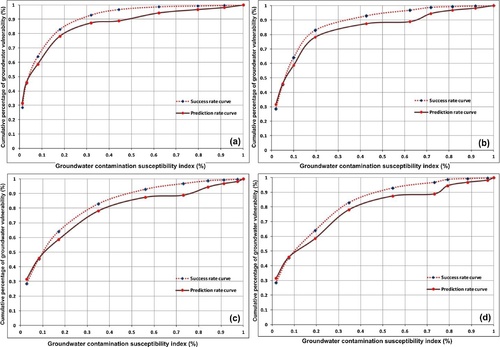
Table 6 AUC of success and prediction rate curve for different models applied.

MODEL applied	AUC (%)
	Success rate	Prediction rate
DRASTIC	89.69	84.54
Modified DRASTIC	87.24	83.02
Pesticide DRASTIC	81.23	75.41
Modified pesticide DRASTIC	81.56	76.03

4.4 Sensitivity analysis

This sensitivity analysis helps to evaluate the desired vulnerability maps and also evaluate its consistency (Saidi et al., 2011). Statistical calculation of results derived from removing only one layer at a time is represented in Table 4 and the vulnerability index resulting by removing one or more layers at a time are represented in Table 5. In multiple map removal analysis, based on the results of Table 3, parameters causing least variation on final output were removed first followed by second least and so on. In the present study, vulnerability index is least sensitive to conductivity. In the context of anthropogenic sources of groundwater pollution, the influence of land use land cover is very low in our study area. This may be attributed to the absence of large-scale industries and factories in the study area.

4.5 Model comparison

The output obtained from the four model applied were compared to each other and the variation in the prediction of vulnerability zones through different models applied. Table 7 represents all the possible combination of map comparison and indicates the variation of less than 50%. The highest similarity in prediction is observed between drastic and modified drastic with a similarity of 97% followed by 75% similarity between pesticide drastic and modified pesticide drastic. Highest discrepancies are observed between modified is observed between modified drastic and pesticide drastic with a difference of 48% in prediction, where approximately 43% corresponds to the difference in venerability prediction of 1 categories higher or lower. This variation is due to the implementation of one extra parameter i.e., land use land cover in pesticide drastic model (Brindha and Elango, 2015).

Table 7 Difference in prediction in vulnerability classes between various models in percentage.

Model compared	Difference in vulnerability classes (%)
	−3	−2	−1	0	1	2	3
Drastic versus modified drastic	00	00	0.32	96.72	2.06	0.87	0.03
Drastic versus pesticide drastic	00	3.30	20.15	52.21	23.19	1.15	00
Drastic versus modified pesticide drastic	00	1.02	21.23	61.58	15.10	1.04	0.03
Modified drastic versus pesticide drastic	0.29	3.92	20.74	51.52	22.41	1.11	00
Modified drastic versus modified pesticide drastic	00	1.05	21.39	63.75	13.74	0.08	00
Pesticide drastic versus modified pesticide drastic	00	00	15.40	75.01	8.72	0.69	0.19

5 Conclusion

It is very crucial and needed to investigate the vulnerability of groundwater aquifer systems. Aquifer systems in our study area are under constant threats from potential pollution source both natural and anthropogenic. Despite threats, the quality of groundwater in the study area is generally good. Contamination of aquifer system does not occur very easily but once the groundwater is already contaminated, it becomes very difficult to combat or remediate aquifer contamination. Sensitivity analysis shows that net recharge is the most influential parameters for groundwater vulnerability followed by aquifer media and impact of the vadose zone. After comparing the outcome of all models applied with the actual groundwater status within the study area, DRASTIC models is observed to be the best model for prediction of groundwater vulnerability in Birbhum with a prediction accuracy of approximately 85%.

Acknowledgements

The author expresses his heartiest gratitude to the DST (project No. SB/ES-687/2013 dated 11.11.2014), Government of India for financial support to the project. The author would also like to thank Central Ground Water Board, Survey of India, and Geological Survey of India for their help and support.

Notes

Peer review under responsibility of National Water Research Center.

Appendix A

Supplementary data

Supplementary data associated with this article can be found, in the online version, at https://doi.org/10.1016/j.wsj.2018.02.003.