Complex temporal climate signals drive the emergence of human water-borne disease

Abstract

Predominantly occurring in developing parts of the world, Buruli ulcer is a severely disabling mycobacterium infection which often leads to extensive necrosis of the skin. While the exact route of transmission remains uncertain, like many tropical diseases, associations with climate have been previously observed and could help identify the causative agent's ecological niche. In this paper, links between changes in rainfall and outbreaks of Buruli ulcer in French Guiana, an ultraperipheral European territory in the northeast of South America, were identified using a combination of statistical tests based on singular spectrum analysis, empirical mode decomposition and cross-wavelet coherence analysis. From this, it was possible to postulate for the first time that outbreaks of Buruli ulcer can be triggered by combinations of rainfall patterns occurring on a long (i.e., several years) and short (i.e., seasonal) temporal scale, in addition to stochastic events driven by the El Niño-Southern Oscillation that may disrupt or interact with these patterns. Long-term forecasting of rainfall trends further suggests the possibility of an upcoming outbreak of Buruli ulcer in French Guiana.

• climate
• coherence analysis
• El Niño/La Niña
• Mycobacterium ulcerans
• rainfall
• singular spectrum analysis
• Southern America

Introduction

The identification of cohering patterns between climate and infectious disease using time series analysis is an important component in understanding the ecological niche of disease causing agents and in predicting future outbreaks. Such correlations can occur with both local and large-scale climatic oscillations.^{1,2,3,4,5,6,7,8,9} The mechanisms behind these relationships often vary and have been attributed both to the direct and indirect effects of changing climate, notably for vector-borne and reservoir-borne diseases for which a component of their life-cycle may be highly sensitive to any rainfall or temperature variation. For example, decreases in precipitation can create pools of stagnant water which are breeding grounds for vectors,^4,10 flooding may cause contamination of surface water and wells through overflow of sewage systems and the failure of septic tanks,¹¹ or the loss of crops or water supplies may cause habitual changes or immunological deterioration in the population.¹² A key problem with time series analysis in long-term datasets is the separation of signals and stochastic noise. Noise can hide cohering patterns, while within a series, there may be a number of competing signals of varying strength. For example, rainfall measures over time have a number of seasonal changes; over a long period, an ecological process such as disease outbreaks may only be linked to changes in one of these components.

Buruli ulcer (BU) is an emerging human skin disease caused by the mycobacterium Mycobacterium ulcerans. Related to high-profile infections tuberculosis and leprosy, prevalence has been increasing in certain developing parts of the world and in some areas, it is more common than its aforementioned relations.¹³ Despite this, knowledge of the infection remains limited. Typically found in moist, tropical areas, the disease can have a devastating impact on its host, causing extensive necrosis of the skin and underlying tissue, often leading to permanent disability if left untreated.^14,15 While the route of infection remains unclear, the bacillus is strongly associated with aquatic environments and incidences of the disease are significantly higher on floodplains, or where people come into continual contact with rivers, ponds, swamps and lakes.^16,17,18 In addition, DNA and cultures of the mycobacterium have been found on, or within numerous aquatic species.^{13,19,20,21,22} This relationship with aquatic systems makes it an interesting candidate to look for coherent patterns with environmental parameters like rainfall and changes in large climatic drivers such as the El Niño-Southern Oscillation (ENSO).

MATERIALS AND METHODS

Environmental and disease data

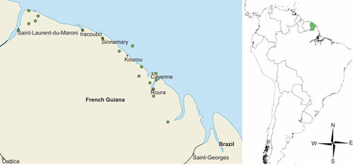
The only accurate long-term (decadal) dataset for cases of BU is from French Guiana in South America, with records going back to 1969. French Guiana also has a well-recorded history of rainfall during this period making it highly suitable for this study. French Guiana is a French ultraperipheral territory bordering the countries of Brazil to the east and south and Suriname to the west. Although large at 83 534 km², the population density is very low with almost all inhabitants located in a thin strip along the coastline. The rest of the country is predominantly pristine primary tropical rain forest and contains the 33 900 km² Guiana Amazonian national park, as well as a wealth of important ecosystems ranging from marshland to coastal mangroves. The numbers of BU cases were obtained from Cayenne Central hospital records dating back to 1969 till 2012, with identification based on a combination of histopathological, microbiological, clinical and genetic analysis. This dataset is the most accurate long-term data on BU to our knowledge, which can be used for coherence with climatic factors. A potential issue with lesion causing diseases is the variation in time between appearance of symptoms and seeking of medical attention, reflected in lesion size. As French Guiana is part of the European Union and is a low-population French territory, case reporting and assessment of lesions incurred a minimal delay; active surveillance of the disease was being undertaken with health-care professionals who are trained to recognize BU being present in all towns and villages. Disease cases are distributed across the territory in line with the distribution of the population and are present almost ubiquitously where there are people. Rainfall data were obtained from Météo-France and were recorded as the average rainfall in millimeters per month from 17 weather stations (Figure 1) across the populated coastal area of the territory from 1969 to 2012. Due to the restricted range of inhabited areas, a small human population and therefore, a relatively low number of cases in each locality, an average rainfall reading from the stations along the coastal area was taken and compared to data on all BU cases across French Guiana. ENSO data for the period were taken from the American National Climatic Data Center and measured as the sea surface temperature (SST) of the equatorial Pacific Ocean.

Figure 1 Map of French Guiana showing the location of 17 weather stations along the coast of French Guiana and the position of French Guiana within South America.

Ethical provisions

Written consent for participation to the study was obtained from patients in all instances. BU cases received treatment appropriately according to the French laws in public health, which are also under application in this territory. The study protocol was authorized by Cayenne General Hospital authorities according to French ethical rules. The database was declared to the Commission National Informatique et Libertés (CNIL NO 3X#02254258) following French law requirements. The database did not include names or any variable that could allow the identification of patients.

Singular spectrum analysis (SSA) decomposition and reconstruction

Since the introduction of SSA by Broomhead and King,^23,24 it has been applied successfully to several economic, financial and industrial time series ^25,26,27 and has also been used previously in the analysis of coherence between disease and climate.^1,6,7,8,28 Consider the real-valued non-zero time series Y_T=(γ₁, γ₂, ..., γ_T) of sufficient length T. The main purpose of SSA is to decompose the original series into a sum of series, so that each component in this sum can be identified as either a trend, periodic or quasiperiodic component (perhaps, amplitude-modulated), or noise. This is followed by a reconstruction of the original series. Each corresponding stage involves two primary steps, for decomposition; embedding and singular value decomposition and for reconstruction; grouping and reconstruction. For a detailed description of each stage, see Golyandina et al (2001).²⁹ In short, decomposition breaks the time series down into its constituent components (in this instance, repeating seasonal and long-term patterns in rainfall). Once isolated, it is possible to identify stochastic noise within the leftover signal and remove it before reconstructing a new noise-free time series.

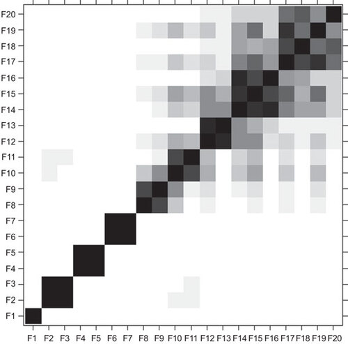
Each seasonal component of the time series was first identified using periodograms, graphical representations of the distribution of power (or variance) among different frequencies. Independence of each seasonal component was also tested. The main concept in studying SSA component properties is ‘separability’, which characterizes how well different components can be separated from each other. SSA decomposition of the series Y_T can only be successful if the resulting additive components of the series are approximately separable. A natural measure of dependence between two time series Y_T⁽¹⁾ and Y_T⁽²⁾ is the weighted correlation or ‘ω-correlation’.²⁹ To identify correlations between all the components within the time series, a ω-correlation matrix was created. This shows the ω-correlation for the components in a 20-grade gray scale from white to black corresponding to the absolute values of correlations from 0 to 1 (with 0 being no correlation and 1 being absolute correlation).

The series was further analyzed using sequential SSA, which refers to an analysis of the residuals.²⁵ As a result of sequential SSA, it is possible to identify signal components which were incorrectly classified as noise through the earlier decomposition and then combine them together in order to build a signal which is shown as total rainfall residual. It is then possible to include the total signal extracted from the residuals in to the earlier reconstruction and use the post-sequential SSA reconstruction for forecasting new data points.

Empirical mode decomposition (EMD)

To explore relationships between seasonal components of the rainfall time series and any corresponding seasonal changes in BU, repeating intra- and inter-annual patterns in BU incidence were extracted using EMD. EMD is a technique developed specifically to decompose non-stationary and nonlinear time series and has been successfully applied to a number of climatic and epidemiological datasets.^1,30 The method is an iterative process which builds a number of oscillatory signals called intrinsic mode functions (IMFs), which are repeatedly subtracted from the time series; each iteration results in an IMF with a longer periodic component until just a trend signal is present. For a detailed description of EMD, see Huang et al.³¹ A periodogram was created for each IMF to assess the frequency of the repeating pattern through time.

Trend coherence analysis

To identify the relationship between the rainfall trend obtained via SSA, SST and the number of human BU cases in French Guiana, continuous wavelet transforms were used. Wavelets have been utilized previously in various branches of ecological theory^{32,33,34,35,36} and to identify relationships between disease and long-term climatic patterns.³⁷ They have the benefit of being unaffected by non-stationary time series, which are often found in ecology.³⁵ Cross-wavelet coherence analysis was performed using the biwavelet R package ³⁸ with the Morlet mother wavelet and 2000 Monte Carlo randomizations. In order to further characterize the association between the time series, phase analysis was also undertaken to identify the phasing difference between the two, for example, whether one precedes the other,³⁹ this is indicated by arrows on the wavelet plots. To further assess the statistical significance of the patterns exhibited by the wavelet approach, null models were tested. To create time series for the null models, bootstrapping was used to construct from the observed time series, control datasets, which share properties of the original series under the following null hypothesis: the variability of the observed time series or the association between two time series is not different to that expected from outbreaks independent of the rainfall trend.

Seasonal coherence analysis

To identify correlations between seasonal components of the rainfall time series extracted via SSA, SST and seasonal changes in BU cases represented by the extracted IMF signals, cross-correlation functions were used.⁴⁰ These measure the similarity between two oscillating time series as a function of a time lag applied to one of them and can be used with stationary time series (i.e., series which statistical properties including mean, variance and autocorrelation are consistent over time).

RESULTS

Singular spectrum analysis

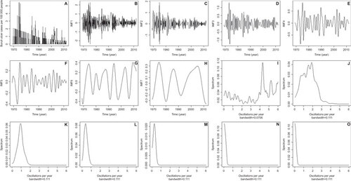
Periodograms of the raw rainfall time series (Figure 2A) identified seasonal components which oscillated yearly for 4-, 6- and 12-month periods (repeating patterns occurring, tri-annually, bi-annually and once per year, Figure 2B) the signals of each repeating oscillation were isolated along with the long-term trend of rainfall (Figure Figures 2C–2F). Remaining data were considered noise and the components were reconstructed into a noise-free signal (2G), a second periodogram of the new reconstructed signal shows the repeating patterns are intact, while stochastic noise has been removed (Figure 2H). Figure 2I shows the resulting output of forecasting from sequential SSA, with rainfall beginning to decline as French Guiana enters a trough of dryer years after several years of high rainfall. The 4-month component corresponds to two rainy seasons, one long rainy season and one short, and also to the main dry season from August to December (Figure 3A). The 6-month bi-annual component corresponds to the two rainy seasons and is a reflection of the strength of these two seasons (Figure 3B), while the 12-month component shows the overall rainfall level for the year (Figure 3C). Separability of these components was confirmed with a ω-correlation matrix showing that these seasonal components did not show high levels of correlation with other components (Figure 4).

Figure 2 Monthly time series data showing the decomposition, reconstruction and forecasting of datapoints using SSA. (A) Original rainfall time series average for 17 weather stations along the coast of French Guiana, from 1969 to 2012. (B) Periodograms of the rainfall time series identifying significant repeating patterns once per year, twice per year and three times per year. SSA extracted component corresponding to periodogram spike of (C) three times per year, 4-month component, (D) twice per year, 6-month component and (E) once per year, 12-month component. (F) The extracted rainfall trend. (G) The reconstructed rainfall time series after the removal of stochastic noise. (H) A second periodogram of the reconstructed rainfall series showing less stochastic noise around the three main repeating patterns. (I) Forecasting of the rainfall trend to 2017 using sequential SSA.

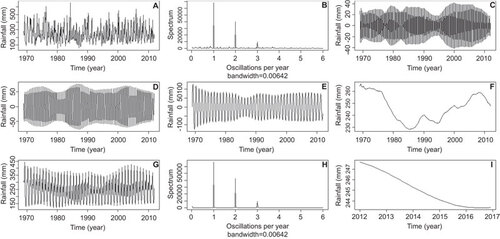
Figure 3 Three-year period of extracted components (dashed line) plotted against the same period of the reconstructed rainfall (solid line), showing which parts of the rainfall series the components represent. (A) Four-month component corresponds to both rainy seasons and the dry season. (B) Six-month component corresponds to the two rainy seasons. (C) Twelve-month component represents the rainfall for the whole year.

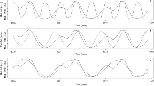
Figure 4 ω-correlation matrix, the F values represent oscillating components within a year (i.e. F6 is the 6-month bi-annual component). The level of correlation can be found by finding the component of interest along the X-axis and looking up the Y-axis to see where it corresponds with other rainfall components. Large values of ω-correlation between reconstructed components indicate that they should possibly be gathered into one group and correspond to the same component in SSA decomposition. The matrix uses a 20-grade gray scale from white to black corresponding to the absolute values of correlations from 0 to 1 (with 0 being no correlation and 1 being absolute correlation).

Empirical mode decomposition

Seven IMF series were produced by EMD of repeating patterns from the BU case data (Figures 5A–5H); periodograms of these show that the first IMF has high levels of variation across the spectrum and therefore, is likely noise, the second is a bi-yearly repeating pattern and the third is a measure of cases per year, the fourth over 2 years and the fifth over 4 years. Subsequent IMF series are long-term trends (Figures 5I–5O).

Figure 5 Monthly time series and EMD of Buruli ulcer cases per 100 000 people. (A) Monthly time series of Buruli ulcer cases per 100 000 people from 1969 to 2012. (B) First IMF. (C) Second IMF. (D) Third IMF. (E) Fourth IMF. (F) Fifth IMF. (G) Sixth IMF. (H) Seventh IMF. Periodograms for (I) first IMF showing a high level of variation across the spectra and therefore, should be considered white noise; (J) second IMF which has its highest power at two cycles per year; (K) third IMF with its highest power at one cycle per year; (L) fourth IMF with the highest power approximately at one cycle every 2 years; (M) fifth IMF with the highest power approximately at one cycle every 4 years; (N) sixth IMF with a low level of cycles representing very long-term trends; (O) seventh IMF also representing long-term trends.

Trend coherence analysis

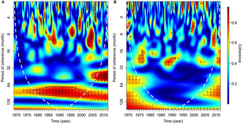
During the period 1969–2012, the series was dominated by four inter-annual peaks in rainfall followed by three inter-annual periods of recessions, with three corresponding peaks and recessions of BU disease cases. The results of the wavelet coherence analyses showed a statistically significant correlation between the two time series for 1979–2000, with cohering peaks and troughs over periods of approximately 8 years (Figure 6A). Phase analysis, indicated by the arrows pointing downwards suggests a preceding relationship of rainfall change occurring before BU cases. In essence, after a peak in rainfall, during a dry period, the number of BU cases increases. Null models showed no significant relationships between rainfall and disease cases. The analysis between cases and SST showed less coherence; however, there were two short periods during the mid-1970s and early 1990s which weakly corresponded (Figure 6B).

Figure 6 Wavelet coherence between (A) Buruli ulcer incidences per 100 000 people and the rainfall trend obtained from SSA. (B) Buruli ulcer incidences per 100 000 people and ENSO. The colors are coded from dark blue to dark red with dark blue representing low coherence through to high coherence with dark red. The solid black lines around areas of red show the α=5% significance levels computed based on 2000 Monte Carlo randomizations. The dotted white lines represent the cone of influence; outside this area, coherence is not considered as it may be influenced by edge effects. The black arrows represent the phase analysis and adhere to the following pattern: arrows pointing to the right mean that rainfall and cases are in phase, arrows pointing to the left mean that they are in antiphase, arrows pointing up mean that cases lead rainfall and arrows pointing down mean that rainfall leads cases.

Seasonal coherence analysis

Cross-correlation functions between the IMF signals representing intra- and inter-annual patterns in BU cases (first, second, third, fourth and fifth IMFs) and both SST and the reconstructed rainfall pattern from SSA analysis showed a number of corresponding signatures.

SST did not correlate with the SSA derived rainfall series (Figure 7A), but did corresponded with rainfall before SSA was applied (Figure 7B), suggesting that SST spikes cause higher levels of unpredictable rainfall anomalies, which during SSA analysis were classified as ‘noise’ or stochastic events. SST also corresponded with the first IMF of BU cases (Figure 7C), which was similarly classified as noise. This may mean that SST creates rainfall anomalies, which cause high levels of BU but do not follow any set seasonal or long-term patterns (i.e., random one off events). SST fluctuations further matched with inter-annual variation of BU cases with long lag periods, suggesting that the total number of cases over these periods is increased by the influence of SST-driven anomalies (Figure Figures 7D–7G). In particular the fourth IMF, where a below average SST (La Niña) value produces a higher than average level of BU cases over 2 years after a lag time of approximately 18 months (7F). Conversely, a peak in SST (El Niño) creates a decline in the 4-year oscillation of BU cases (Figure 7G).

Figure 7 Cross-correlation analysis between (A) ENSO and reconstructed rainfall time series from SSA. (B) ENSO and original rainfall time series. ENSO and (C) first IMF from Buruli ulcer cases, (D) second IMF, (E) third IMF, (F) fourth IMF, (G) fifth IMF. Reconstructed rainfall series and (H) first IMF; (I) second IMF; (J) third IMF; (K) fourth IMF; (L) fifth IMF. Dashed horizontal blue lines in all panels represent the 95% confidence limit; black vertical lines which go beyond the dashed line can be considered non-random cohering oscillations between the two time series being assessed, with the lag period between an above average oscillation in the first time series and a subsequent above average oscillation in the second shown on the X-axis.

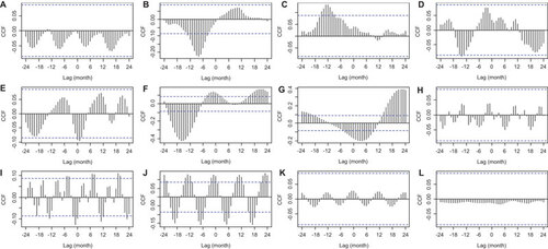
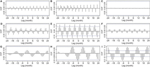
The reconstructed rainfall series has a corresponding relationship with both the second and third IMF (Figure Figures 7I and 7J), suggesting that an above average level of precipitation contributes to an above average spike in bi-annual BU cases, and also the overall yearly number of cases. By looking at the SSA-derived components of rainfall against the IMF signatures of BU, it is possible to identify the exact rainfall components which are driving these spikes. The SSA-derived 4-month component correlated with no IMF signatures (Figures 8A–8C). Figures 8D–8F show the correlations of the first, second and third IMF signatures with the SSA-derived 6-month component (i.e., the strength of both the two wet seasons); a significant correlation is identified with the bi-annual BU cases (second IMF) with an approximate 5-month lag; therefore, because of the average reported incubation periods of 3–5 months⁴¹ and the lag time of several weeks before diagnosis, the two spikes in cases per year are most likely to be driven by the strength of the two spikes in rainfall per year rather than the two dry seasons. The 12-month component which is a measure of the total rainfall per year did not correlate with any seasonal IMF signatures (Figures 8G and 8H), but as expected correlated with the overall level of BU per year (8I).

Figure 8 Cross-correlation analysis between rainfall seasonal components extracted by SSA and seasonal IMF series of Buruli ulcer. Four-month component and (A) first IMF, (B) second IMF, (C) third IMF. Six-month component and (D) first IMF, (E) Second IMF, (F) third IMF. Twelve-month component and (G) first IMF, (H) second IMF, (I) third IMF. Dashed horizontal blue lines in all panels represent the 95% confidence limit; black vertical lines which go beyond the dashed line can be considered non-random cohering oscillations between the two time series being assessed, with the lag period between an above average oscillation in the first time series and a subsequent above average oscillation in the second shown on the X-axis.

DISCUSSION

The identification of more than one temporal correlation between rainfall and BU disease, in addition to wet weather anomalies outside of usual seasonal peaks in rainfall being driven by SST, highlights the complexity of using environmental changes in predicting disease outbreaks. The stochastic SST-driven incidences and the influence of long-term rainfall in addition to seasonal drivers is a first for BU in the world. While a similar long- and short-term climatic pattern has already been linked to cholera outbreaks,^28,42 the results of this paper show that such patterns are likely to be more spread among aquatic infectious pathogens such as with M. ulcerans and that SST relationships may be driving stochastic cases.

While further study will be required to fully understand what niche M. ulcerans occupies within French Guiana, in this paper, the identification of a relationship with rainfall provides important testable insights into its disease ecology. It also exemplifies the importance of using long-term datasets when trying to establish relationships between the environment and infectious disease, and the use of techniques such as wavelets, SSA and EMD to look deeper into time series.

By removing noise and decomposing the time series using SSA, it was possible to look at the influence of each individual seasonal pattern on BU and to identify a cause of important rainfall anomalies, which occur outside the regular seasonal patterns. By further extracting a long-term trend and relating this to cases, the effects of several components of rainfall become apparent, something which would perhaps be lost without decomposition.

During the analysis, EMD had some advantages and disadvantages over SSA, which makes it suitable for differing time series, dependent on the application. In this instance, the ability to successfully identify noise and a seasonal component, in addition to a hierarchy of increasing long-term periodic components in disease cases, was beneficial, particularly when linking disease patterns to SST. SSA, however, provided a more accurate separation of seasonal components within the rainfall data.

The increasing use of wavelets^{32,33,34,35,37} is an important development for time series analysis in epidemiology; previously in this field, non-stationarity presented a serious problem for relating ecological, epidemiological and climatic datasets.^43,44,45 Wavelets provide the advantage of being localized in both time and frequency, whereas the standard Fourier transform, traditionally used in time series analysis, is only localized in frequency,³⁵ which, although useful for identifying constant periodic components, is not able to account for changes in frequency over time.

The results of the relationship between SST and BU cases broadly agrees with similar observations in Australia where it was found that periods of wet weather approximately 16–17 months prior to an outbreak, followed by a period of dry weather for 5 months to be the most suitable for BU emergence.⁴⁶ The results presented here suggest that outbreaks of BU over a long period (at least 2 years, as represented by the fourth IMF), correspond with a decline in SST (i.e., a La Niña event) 17 months prior, while the opposite is true for El Niño, with the effect causing a below average decrease in BU cases over the preceding 4 years. A La Niña event in the north of South America corresponds to a marked increase in wet weather anomalies (as corroborated by the significant cross-correlation function between the pre-SSA rainfall and SST), while El-Niño signals an increase in dryer weather. As SST also correlates with high rainfall events and BU cases classified as stochastic, it is possible that SST driven rainfall anomalies create random outbreaks in BU, independent of the usual seasonal cycles over a 2-year period.

The long-term and seasonal relationships between rainfall and cases, i.e., the long-term peaks in BU driven by a recession in rainfall over several years, and the bi-annual peaks in cases driven by spikes in the two rainy seasons, could be explained in several ways. While the limited knowledge of BU disease transmission makes it only possible to speculate, the analysis does present an opportunity to shed further light on the ecological niche occupied by M. ulcerans and its environmental heterogeneity in space and time. Long periods of wet weather followed by a decrease in rainfall may increase the number of stagnant water bodies and swampland, flowing rivers may recede into a series of isolated pools,⁴⁷ while newly formed channels and wetlands will be cut off. This could spark an outbreak of disease vectors, host carriers and other aquatic species that have been identified to have a relationship with BU and which thrive in these conditions,^{19,22,48,49,50} or beneficially change the aquatic community structure. A second hypothesis, which assumes that the disease agent does not necessarily require a true symbiotic relationship, would be that the initial rainfall washes the agent into new territory, and once established, the dry weather will again increase the number of preferential water bodies, thereby increasing the number of cases. Both events have the potential to cooccur over a long and short period of time and could potentially be working at differing spatial scales, driven by either long- or short-term rainfall patterns. Previous studies have shown how community assemblages and system dynamics can be significantly altered over varying periods of time at sites with differing sizes, hydrologies and landscape parameters.^{18,51,52,53,54,55} The majority of the BU cases occur when both the long- and short-term temporal changes coincide, suggesting weather conducive to providing an increase in infectious habitats or human contact with these habitats during such a period. Using the argument that the disease agent is most abundant in stagnant water, it is possible to hypothesize that large bodies of water created after several years of high rainfall may recede slowly, stagnate and undergo significant changes in biotic community over several dry years. Nested within this period, high peaks in rainy seasons as suggested by an increase in the biannual component, or SST-driven rainfall anomalies, will cause these stagnating areas to swell, potentially flooding or seeping onto pathways where human contact is increased. In addition, periods of high rainfall during periods of long-term dryer climates could also be conducive to the occurrence of potential invertebrate vectors. Previous work on mosquito populations, for example, which have been linked to BU,⁴⁸ shows that they are at their highest during periods of high short-term climatic variability, cited as the amount of short-term fluctuations around a mean climate state on a fine time scale.^3,56,57,58 This may add weight to the idea of mosquito-based vectors, although it is possible that several less studied aquatic species exhibit similar responses. It must also be considered that the relationship could be influenced more by human behavior, for example, dryer years will often induce an increase in recreational use of local water bodies, notably for fishing and hunting.

The results of the forecasting are of potential importance in predicting future disease emergence. The most recent highest rainfall in French Guiana has occurred in 2009 and it is being followed by a 5-year period of dry weather (Figure 2I). Based on the analysis and the identification of a relationship with rainfall, it is possible to predict that this should also be followed by an increase in BU cases in the region.

Caution must be expressed when using time series data, particularly over long periods, as changes in diagnostic capabilities (for example, the introduction of polymerase chain reaction techniques allowing accurate genetic ifentification of the bacteria, knowledge of the disease and improvements in equipment and recording) and the accuracy in weather data collection will cause significant temporal discrepancies. These factors are difficult to address and are inherent to all such studies. It is also important to note that unpredictable external factors such as socioeconomical changes can also be having an unknown influence. The use of long-term weather data also presents the problem of how to include landscape parameters, as these also have an influence on a disease, but are often not available or poorly recorded early on in time. In this instance, however, it seems unlikely that a cyclical pattern is related to a steady change in population and landscape. The robust analysis shows that French Guiana time series for BU cases reveals interesting non-random patterns, which are vital for understanding the ecological niche of this aquatic microbial agent.

This work was supported by Aaron Morris, Rodolphe E Gozlan, Pierre Couppié and Jean-François Guégan, who have benefited from an ‘Investissement d’Avenir’ grant managed by Agence Nationale de la Recherche called LabEx CEBA (Centre d'Etude sur la Biodiversit′ Amazonienne) (ref. ANR-10-LABX-2501). This work was partially supported by a grant from ANR EREMIBA (05 SEST 008-02). Jean-François Guégan is sponsored by the Institut de Recherche pour le Développement and the Centre National de la Recherche Scientifique. This work has benefited from a PhD studentship awarded to Aaron Morris from the Bournemouth University.