On the categorization of demand patterns

Abstract

The categorization of alternative demand patterns facilitates the selection of a forecasting method and it is an essential element of many inventory control software packages. The common practice in the inventory control software industry is to arbitrarily categorize those demand patterns and then proceed to select an estimation procedure and optimize the forecast parameters. Alternatively, forecasting methods can be directly compared, based on some theoretically quantified error measure, for the purpose of establishing regions of superior performance and then define the demand patterns based on the results. It is this approach that is discussed in this paper and its application is demonstrated by considering EWMA, Croston's method and an alternative to Croston's estimator developed by the first two authors of this paper. Comparison results are based on a theoretical analysis of the mean square error due to its mathematically tractable nature. The categorization rules proposed are expressed in terms of the average inter-demand interval and the squared coefficient of variation of demand sizes. The validity of the results is tested on 3000 real-intermittent demand data series coming from the automotive industry.

Keywords:

• categorization
• forecasting
• inventory control
• intermittent demand

Introduction

The categorization of alternative demand patterns is an essential element of many inventory control software packages. The common practice in the software industry is to arbitrarily categorize demand patterns and then select an estimation procedure and stock control method in order to forecast future requirements and manage stock efficiently. For example, certain arbitrary cutoff values may be given to the number of demand occurring periods in a year, average demand per unit time period and standard deviation of the demand sizes in order to define demand patterns as slow, intermittent, lumpy, fast, etc.

In this paper, we are concerned with the selection of the most appropriate estimation procedure as a first step towards a more systematic and meaningful approach to the categorization problem.

Typically, for fast moving items, analysis of the demand data series will lead to the selection of an appropriate forecasting model (or a class of models) and optimization of the forecast parameters will be based on minimizing the mean square error (MSE), Bayesian recursion or some form of residual auto-correlation analysis. For the remainder of the categories Moving Averages, simple Exponentially Weighted Moving Averages (EWMA) or Croston's method¹ are the most commonly chosen estimation procedures. In the case of the sporadic and/or irregular demand patterns, the sparseness of data and/or the aggregate policies required, may result in an empirical determination of the control parameters, so that, for example, a 13-period Moving Average or a smoothing constant equal to 0.15 are specified across a whole category.

Re-categorization occurs at fixed time intervals (annually for example) and the sensitivity of the categorization rules to outliers is usually examined so that the categorization scheme does not allow products to move from one category to the other simply because a few extreme observations have been recorded. Logical inconsistencies are also explored so that demand for a stock keeping unit (SKU) is always classified in the intended category. However, the more consistent the categorization scheme is, the greater the number of the demand categories that need to be considered. Theoretical and practical requirements that should be taken into account when developing rules for the purpose of distinguishing between alternative demand patterns have been discussed in Williams.²

Ultimately, the objective of the categorization exercise is the selection of the most appropriate estimation procedure. However, if this is the real objective it seems more meaningful to compare possible forecasting methods for the purpose of establishing regions of superior performance and then categorize the demand patterns based on the results. The theoretical comparisons need to be based on an accuracy measure, and the MSE is the most obvious candidate because of its mathematically tractable nature. Direct comparison of the theoretical MSEs, over a fixed lead time, associated with any two estimation procedures will result in establishing rules that indicate regions of superior performance of one method over the other. When there are more than two estimators taken into account there will be some overlapping areas regarding superior performance and the analysis will need to be extended in order to propose rules which are valid across all methods.

We demonstrate our approach by considering three methods: (a) Croston's method, that has been specifically designed to deal with intermittence, (b) an alternative to Croston's estimator, developed by the first two authors of this paper and (c) the more generally applicable EWMA. The categorization rules are expressed in terms of the series' average inter-demand interval and the squared coefficient of variation of the demand sizes (when demand occurs). The validity of our results is tested on 3000 real-intermittent demand data series.

Categorization schemes proposed in the literature

Williams² proposed a method of categorization of demand patterns based on an idea that is called variance partition (we split the variance of the demand during lead time into its constituent parts). The purpose of categorization was the identification of the most appropriate forecasting and inventory control methods for the resulting categories.

Categorization of the items takes place in accordance with the matrix shown in Figure 1 (with the cutoff values being the result of managerial decision).

Figure 1 Williams' categorization scheme.

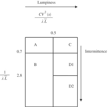
In the matrix shown below, λ is the mean (Poisson) demand arrival rate, L̄ the mean lead time duration and CV²(x) the squared coefficient of variation of demand sizes. 1/λL̄ indicates the number of lead times between successive demands (how often demand occurs or how intermittent demand is). The higher the ratio, the more intermittent demand is. CV² (x)/λL̄ indicates how lumpy demand is. Lumpiness depends on both the intermittence and the variability of the demand size, when demand occurs. The higher the ratio the more lumpy demand is: category D1—sporadic (lumpy); category D2—highly sporadic (lumpy). In that case we have few very irregular transactions accompanied by highly variable demand sizes; category B—slow moving; others—smooth.

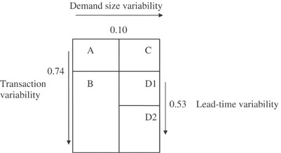
Eaves³ analysed demand data from the Royal Air Force (RAF) and concluded that Williams' conceptual classification scheme did not adequately describe the observed demand structure. In particular, it was not considered sufficient to distinguish a smooth demand pattern from the remainder simply on the basis of the transaction variability. Consequently, a revised classification scheme was proposed (see Figure 2) that categorizes demand based on the variability of the transactions' rate, demand size variability and lead time variability. The line items with low transaction variability are sub-divided into smooth and irregular according to the demand size variability. The smooth and slow-moving demand categories are distinguished from the rest based on the variance of the demand sizes, and the lead time variance is used only for distinguishing between erratic and highly erratic demand. The cutoff values were decided based on: (a) the characteristics of the particular demand data set and (b) sufficient sub-sample (within each demand class) size considerations. In particular, the cutoff points were as follows: transaction variability—0.74; demand size variability—0.10; lead time variability—0.53. Category A—smooth; category C—irregular; category B—slow-moving; category D1—erratic; category D2—highly erratic.

Figure 2 Eaves' categorization scheme.

The above-discussed categorization schemes are the only ones to appear in the academic literature that take into consideration alternative demand patterns and consequently distinguish between them for the purpose of selecting the most appropriate forecasting (and stock control) procedure. Nevertheless, the cutoff values have been arbitrarily chosen so that they make sense only for the particular empirical situations that were analysed in the corresponding pieces of research.

There is no doubt that the criteria used for categorization are meaningful. In fact, similar criteria will be used for the categorization rules that will be proposed later on in this paper (with the difference that lead times are assumed to be constant). It is rather the arbitrary cutoff values assigned to them that create certain doubts about the potential applicability of the proposed categorization schemes to any different possible context.

An alternative approach to the demand categorization problem

Johnston and Boylan⁴ compared Croston's intermittent demand estimation procedure with EWMA on theoretically generated demand data over a wide range of possible conditions. (Croston's approach to forecasting intermittent demand and the latest research findings regarding his method are presented in Appendix A). Many different average inter-demand intervals (negative exponential distribution), smoothing constant values, lead times and distributions of the size of demand (negative exponential, Erlang and rectangular), were considered. The comparison exercise was extended to cover not only Poisson but also Erlang demand processes. The results were reported in the form of the ratio of the MSE of one method over that of the other. For the different factor combinations used in this simulation experiment, Croston's method was superior to EWMA for inter-demand intervals greater than 1.25 review periods. This result was the first response to the question raised in Anders Segerstedt's paper:⁵ ‘When is best to separate the forecasts like Croston suggests and when is it best with traditional treatment (ie simple exponential smoothing)?’.

Definition of intermittent demand now results from a direct comparison of possible estimation procedures so that regions of relative performance can be identified. It seems more logical indeed working in the following way:

1. Compare alternative estimation procedures.

2. Identify the regions of superior performance for each one of them.

3. Define the demand patterns based on the methods' comparative performance rather than arbitrarily defining demand patterns and then testing which estimation procedure performs best on each particular demand category.

The approach discussed above is taken forward in the research described in this paper, in that the decision rules will be the outcome of a comparison between MSE performances. There are some significant differences though which are the following: (a) the fact that theoretical rather than simulated MSEs are considered, (b) we propose a two, rather than one, parameter classification scheme, taking into account not only the demand interval but also the demand size variability and (c) we validate empirically our results.

MSE is similar to the statistical measure of the variance of forecast errors (which consists of the variance of the estimates produced by the forecasting method under concern and the variance of the actual demand) but is not quite the same since bias can also be explicitly considered. MSE is a quadratic error measure and as such it may be unduly influenced by outliers but it is the only accuracy measure that allows theoretical results to be tested in practice. In addition, MSE can be defined for all demand data series rather than ratio-scaled data only, an issue that is obviously of great importance in an intermittent demand context.

The lead time MSE assuming error auto-correlation

In an inventory control application, the forecast errors produced by any estimation procedure are usually assumed to be normal and independent (or Poisson for slow moving items). Usually the effect of non-normality is small. ‘However, for lead times greater than 1 the errors will typically be auto-correlated and this issue (the issue of auto-correlation of the forecast errors) has received very limited attention’.⁶

By ignoring the auto-correlation term, we are most probably overstating the performance of the estimation procedures under concern since auto-correlations induced by bias or lumpiness are generally positive.

The MSE over a fixed lead time of duration L, assuming error auto-correlation, for unbiased forecasting methods is calculated as follows:⁷where the variance terms on the right-hand side refer to a single period.

For any biased demand estimation procedure, it is easy to show that the lead-time MSE is given by (2):

It immediately follows, from Equation (2), that the MSE over lead time L for method A is greater than the MSE over lead time L for method B if and only if where the subscripts refer to the forecasting methods employed.

The MSE of intermittent demand estimation procedures

Croston¹ showed that the performance of EWMA on intermittent demand data series depends heavily on which points in time are considered. That is, if all the estimates produced by the method, at the end of every forecast review period, are taken into account, the method is unbiased whereas a certain bias should always be expected when we isolate the estimates made only after a demand occurring period. The former scenario corresponds to a re-order interval (periodic review) system while the latter to a re-order level (continuous review) system. Moreover, the variance of the estimates produced by EWMA in those two cases is not the same. The sampling error of the mean associated with this method is always higher when we consider all points in time.

Regarding Croston's estimator (see Appendix A), the performance of the method is independent of which points in time are considered. Croston's method has been claimed to be unbiased and of great value to manufacturers forecasting intermittent demand. The method is widely used in industry and it is incorporated in best-selling forecasting (and stock control) software packages. A rather disappointing empirical performance of this estimator, though, has been reported in the academic literature^{8, 9} when compared with conceptually simpler estimators, such as EWMA or even simple moving averages. These findings have motivated research, conducted by the first two authors of this paper, on the theoretical properties of Croston's method. Syntetos and Boylan¹⁰ showed that Croston's estimator is biased. Based on Croston's approach and theoretical model (demand is assumed to occur as a Bernoulli process and therefore the inter-demand intervals are geometrically distributed) the same authors¹¹ proposed a modification on Croston's method that is approximately unbiased where p_t′ is the exponentially smoothed inter-demand interval, updated only if demand occurs in period t, z_t′ the exponentially smoothed size of demand, updated only if demand occurs in period t, α the common smoothing constant value used and Y_t′ the estimate of demand in unit time period t.

The method's performance is independent of which points in time are considered and its theoretical properties are also discussed in Appendix A.

For the purpose of illustrating our approach, we proceed by referring to the case of the periodic review systems (ie we consider all points in time) since such systems are most often used in practice for the management of intermittent demand items.^{3, 9} At this point, we need to mention that issue point forecasts could also be relevant in the context of a periodic review system if stock is reviewed at the end of each period in which a forecast is made. Hence, even if we restrict our attention to periodic review systems, both ‘all points in time’ and ‘issue points’ should be considered. Nevertheless, only the former scenario will be explored in this paper.

Considering results presented in the academic literature^{1, 10, 11, 12} the MSE over a fixed lead time L associated with EWMA, Croston's method and Syntetos and Boylan method (elsewhere referred to also as the ‘Approximation’ method^{3, 11, 12, 13}), when all points in time are considered, is calculated as follows: where α is the common smoothing constant value used, with β=1−α. In case of Croston's and Syntetos and Boylan method, the α value is the smoothing constant value used for the intervals. Following Croston's¹ suggestion the same smoothing constant is also used for demand sizes although, following the suggestion of Schultz,¹⁴ a different smoothing constant could also be used. μ and σ² are the mean and variance, respectively, of the demand sizes, when demand occurs, and p is the average inter-demand interval expressed in number of forecast review periods (including the demand occurring period).

Equation (5) and approximations (6) and (7) are based on the assumption that demand occurs as a Bernoulli process and therefore the inter-demand intervals are geometrically distributed (see also Appendix A).

Theoretical comparisons of the MSEs

We start the analysis by assuming that the approximated or exact MSE of one method is greater than the approximated or exact MSE of one other method, and we try to specify under what conditions the inequality under concern is valid. Considering inequality (3) it is obvious that the comparison between any two estimation procedures is only in terms of the bias and the variance of the one step ahead estimates associated with their application. That is, the length of the fixed lead time and the variance of demand itself do not affect the final results.

At this point, it is important to note that all the pairwise comparison results are generated assuming that the same smoothing constant value is employed by all of the estimation procedures under concern. We recognize that the use of the same smoothing constant may put one or more methods at a relative advantage/disadvantage but the issue of sensitivity of the comparative performance results to the application of the same α value has not been further explored.

Comparison results (MSE Croston's method–MSE Syntetos and Boylan method)

We first compare the MSE of Croston's method with that of the Syntetos and Boylan method over a fixed lead time of length L (L⩾1): for p>1, 0⩽α⩽1.

(All detailed derivations of our results are available upon request from the first author.)

The theoretical rule developed above is expressed in terms of the squared coefficient of variation (CV²) and the average inter-demand interval. The rule can then be further analysed (considering different possible values of the control parameters: α, μ, p and σ²) so that cut-off values can be determined.

For any p>1.32, inequality (8) holds (superior performance is theoretically expected by the new method). For p⩽1.32

• If CV²>0.48 then MSE_CROSTON>MSE_{SYNTETOS&BOYLAN}

• If CV²⩽0.48, then there is a p cutoff value (1<p⩽1.32) below which Croston's method performs better (ie the inequality is not valid). For example if CV²=0.15, then the cutoff value is p=1.20. For 1<p⩽1.20, Croston's method performs better and for p>1.20 the Syntetos and Boylan method performs better.

As the ratio CV² decreases, the p cutoff value increases, and for CV²=0.001 the cutoff value is p=1.32, therefore, Croston's method performs better for 1<p⩽1.32.

The above results are valid for α=0.15 and approximately true for other realistic α values (refer to Table 1).

Table 1 MSE Croston's method–MSE Syntetos and Boylan method

αSmoothing constant value	p-Cutoff value	CV^2cutoff value
0.05	1.32	0.49
0.10	1.32	0.49
0.15	1.32	0.48
0.20	1.31	0.47

From the above analysis, it is clear that there are four decision areas in which one method can be theoretically shown to perform better than the other. For average inter-demand intervals and squared coefficients of variation above their corresponding cutoff values, we know with certainty which method is theoretically expected to perform better. The same happens when either of the criteria takes a value above its cutoff value, while the other takes a value below its cutoff value. The only area that requires further examination is the one formed when both criteria take a value below their corresponding cutoff values.

From Table 1 we can conclude that for all smoothing constant values that are likely to be applied in practice, the new method should always perform better than Croston's method for any p>1.32 unit time periods and/or CV²>0.49.

In the area that corresponds to p⩽1.32 and CV²⩽0.49, neither method can be theoretically shown to perform better in all cases. Our numerical analysis resulted to assigning this area of indecision to Croston's method. (In the majority of cases Croston's method performs better or if this is not the case the differences are so small that we are almost indifferent as to which estimator will be used.) Similarly, for the EWMA—Syntetos and Boylan method comparison, the corresponding area will be assigned to the method that performs worse in the other decision areas. Clearly, the derivation of a function, based on which the more accurate estimator can be exactly identified, would be welcomed, but such an exercise is beyond the scope of this research.

Our categorization scheme is as indicated below (Figure 3).

Figure 3 Cutoff values (Croston's method–Syntetos and Boylan method).

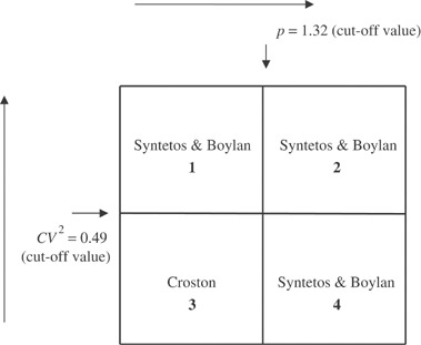
The corresponding demand categories are as follows: area 1—erratic (but not very intermittent); area 2—lumpy; area 3—smooth; area 4—intermittent (but not very erratic).

Comparison results (MSE EWMA–MSE Syntetos and Boylan method)

MSE_EWMA>MSE_{SYNTETOS&BOYLAN} if and only if for p>1, 0⩽α⩽1.

An analysis similar to that presented in the previous sub-section reveals that for smoothing constant values that are commonly applied in practice, the Syntetos and Boylan method should always perform better than the EWMA method for any p>1.20 unit time periods and/or CV²>0.49.

Comparison results (MSE EWMA–MSE Croston's method)

if and only if

But

This is indeed an unexpected result if we consider the unbiased nature of EWMA when all points in time are considered. The theoretical explanation is the high sampling error of the mean of EWMA, but the result may also be explained in terms of the approximate nature of Croston's MSE.

The results of the above-discussed pairwise comparisons indicate that if all points in time are considered, then one of the estimation procedures specifically designed to deal with intermittence could be utilized for all SKUs. For fast demand items, the Syntetos and Boylan method's performance is in general though inferior to that of Croston's method. The opposite is the case when more intermittent and/or more irregular demand patterns are considered.

Overall comparison results

When all points in time are considered, the Syntetos and Boylan method performs better than the other two methods for p>1.32 and/or CV²>0.49. For p⩽1.32 and CV²⩽0.49, Croston's method is theoretically expected to perform better than the other methods. This result is, at least intuitively, not what one may expect and it is attributed to the large variance associated with the estimates produced by EWMA.

Simulation exercise

A sample of 3000 files is available for the purpose of this research. Each file consists of 24 demand time periods/months. The average inter-demand interval ranges from 1.04 to 2 months and the average demand per unit time period from 0.5 to 120. The average demand size, when demand occurs, is between 1 and 194 units and the variance of the demand sizes between 0 and 49 612 (the squared coefficient of variation ranges from 0 to 14). That is the sample contains: slow movers; intermittent demand series with a constant, or approximately constant, size of demand; and very lumpy demand series. What follows is the number of files that falls within each of the four classes of demand that result from our classification scheme: erratic (but not very intermittent)—441 files; lumpy—314 files; smooth—1271 files; intermittent (but not very erratic)—974 files.

To initialize a particular method's application, the first 13-period demand data are used. Therefore, the out-of-sample comparison results that are reported in this paper will refer to the latest 11 monthly demand data. The first EWMA estimate is taken to be the average demand over the first 13 periods. In a similar way, the first exponentially smoothed estimate of demand size and inter-demand interval can be based on the average corresponding values over the first 13 periods. If no demand occurs in the first 13 periods, the initial EWMA estimate is set to zero and the inter-demand interval estimate to 13. As far as the demand size is concerned, it is more reasonable to assign an initial estimate of 1 rather than 0. Optimization of the smoothing constant values used was not considered because of the very few (if any) demand occurring periods in the data sub-set withheld for initialization purposes. Since the available data series were so short (24 periods), the initialization effect is carried forward by all estimators on all out-of-sample point estimates. Clearly, longer demand data series would have been welcomed. However, longer histories of data are not necessarily available in real-world applications. Decisions often need to be made considering samples similar to the one used for this research.

The smoothing constant value is introduced as a control parameter. In an intermittent demand context, low smoothing constant values are recommended in the literature. Smoothing constant values in the range 0.05–0.2 are viewed as realistic.^{1, 4, 8} From an empirical perspective, this range covers the usual values of practical usage. In this research four values are simulated: 0.05, 0.10, 0.15 and 0.20.

The lead time is also introduced as a control parameter. The lead times considered are 1, 3 and 5 periods.

MSE results

A χ²-test was decided to be the most appropriate way of assessing the validity of the theoretical rules proposed in the previous section. The average inter-demand interval and the squared coefficient of variation of the demand sizes were generated for all 3000 files and the proposed categorization rules were used in order to indicate which method is theoretically expected to perform better or best in each one of those files. The null hypothesis developed is that the performance of the methods is independent of what is expected from the theory.

Croston's method is always (on every demand data series) expected to perform better than EWMA, independently of the demand data series characteristics. As such, the Z-test statistic for the population proportion will be used to test whether or not the number of files on which Croston's method out-performs EWMA is significantly greater from the number of files on which EWMA performs better.

For testing the categorization rule regarding all methods' performance a 3 × 2 (2 degrees of freedom) or 4 × 2 (3 degrees of freedom) table will be used depending on whether or not ties occur.

The χ²-test statistic values are indicated, for different smoothing constant values, in Table 2. In brackets we present the number of files that the methods perform as expected. The shaded area refers to the Croston—EWMA pairwise comparison and the values presented are the Z-test statistic values for the population proportion. Statistically significant results at 1% level are emboldened while significance at 5% level is presented in italics.

Table 2 χ² test results

α	L.T.	Croston-EWMA	EWMA-S.B.^a	Croston-S.B.^a	Overall categorization rules

^aS.B. stands for Syntetos and Boylan method.

The results generated on MSEs indicate the practical validity of the rules proposed in this paper. The performance of the methods is clearly not independent of what the categorization rules suggest. This is true at a pairwise comparison level and when the overall rule (regarding all methods' performance) is considered. The results, though regarding the EWMA—Croston comparison, are not what one may have expected empirically for the ‘smoother’ SKUs.

There is some empirical evidence to attribute that difference to the high variability of the errors produced by the EWMA estimator.¹² The decomposition of the empirical MSE into its constituent components (bias squared+variability of demand+variability of the estimates) would obviously enable the rigorous assessment of the contribution of these components to the empirical MSE. Nevertheless, no such results have been generated in our empirical study and this issue requires further simulations on real data.

Conclusions

The categorization of alternative demand patterns facilitates the selection of a forecasting method and it is an essential element of many inventory control software packages. Despite the importance of this issue though, the problem of categorizing demand patterns has received very limited attention so far in the academic literature. Some work has been performed in this area, which nevertheless lacks either universal applicability or empirical validation of the results.

The common practice in inventory control software industry is to arbitrarily categorize demand patterns and then select an estimation procedure in order to forecast future requirements and manage stock efficiently. Ultimately, the objective is the selection of a forecasting method. Based on Johnston and Boylan⁴ we propose an alternative approach to the categorization problem according to which direct comparison of the forecasting methods results in specifying the demand categories. The pairwise comparisons are based on the theoretical MSEs and they can indicate universally valid regions of expected superiority of one method over the other. We illustrate our approach by considering Croston's method, Syntetos and Boylan method and EWMA. The validity of the rules proposed is confirmed by means of simulation on 3000 real-intermittent demand data series. The empirical results also demonstrate the lack of sensitivity of the cutoff points proposed to the smoothing constant value being used.

The resulting categories of any demand classification scheme for inventory management are ultimately meant to serve the inventory objectives of improved customer service levels and/or reduction of stock holdings. In that respect the forecast accuracy of an estimator (and subsequently its bias, or the lack of it, and its sampling error of the mean) is not the only theoretical and practical concern regarding categorization. That is to say, specific demand distributional assumptions as well as certain stock control models should also, eventually, be considered. As far as the former issue is concerned, it is important to note that an interesting avenue for further research could also be the comparison of non-parametric (bootstrapping) versus parametric approaches, the latter comprising a forecasting method and a particular assumed demand distribution. The coefficient of variation of demand sizes has been shown in this paper to be very important from a forecasting perspective. Nevertheless, we should mention that the use of this criterion also implies the non-compliance of the true demand size distribution with standard theoretical distributions (such as the geometric or the logarithmic). As the coefficient of variation rises, so it becomes more difficult to justify the use of any standard distribution and that, as pointed out before, opens up a further avenue of research: under what circumstances should a distributional approach be used at all. What has been presented in this paper can be perceived as only a first step towards a more systematic and meaningful approach to the categorization problem.

Appendix A: Croston's method, Syntetos and Boylan method

Croston,¹ as corrected by Rao,¹⁵ proved the inappropriateness of exponential smoothing and he also expressed, in a quantitative form, the bias associated with the use of this method, when dealing with intermittent demands.

Moreover, assuming a stochastic model of arrival and size of demand, Croston introduced a new method for characterising the demand per period by modelling the demand in one period from constituent events.

According to his method, separate exponential smoothing estimates of the average size of the demand and the average interval between demand incidences are made after demand occurs. If no demand occurs the estimates remain exactly the same.

Let: 1/p_t be the Bernoulli probability of demand occurring in period t; p_t the geometrically distributed (including the first success, ie demand occurring period) inter-demand interval; p_t′ the exponentially smoothed inter-demand interval, updated only if demand occurs in period t, E(p_t)=E(p_t′)=p; z_t the normally distributed demand size, when demand occurs; z_t′ the exponentially smoothed size of demand, updated only if demand occurs in period t, E(z_t)=E(z_t′)=μ; α the common smoothing constant value used and Y_t the demand in unit time period t.

Under these conditions the expected demand per unit time period is E(Y_t)=μ/p. Following Croston's estimation procedure, the forecast, Y_t^′ for the next time period is given by: Y_t′=z_t′/p_t′ and, according to Croston, the expected estimate of demand per period in that case would be: E(Y_t′)=E(z_t′/p_t′)=E(z_t′)/E(p_t′)=μ/p (ie the method is unbiased).

The variance of the forecasts produced by this method is calculated by Croston as follows:

Syntetos and Boylan¹¹ showed that Croston's method is biased and that the expected estimate of demand per unit time period is not as calculated by Croston, but rather

Moreover, the sampling error of the mean was also found to be different:

The researchers proposed a new estimator that takes into account the smoothing constant value used and which is the following:

The expected estimate of demand per unit time period as well as the variance of the estimates produced by this method are given by (A.5) and (A.6), respectively

References

- CrostonJDForecasting and stock control for intermittent demandsOpl Res Q19722328930410.1057/jors.1972.50
- WilliamsTMStock control with sporadic and slow-moving demandJ Opl Res Soc19843593994810.1057/jors.1984.185
- EavesAHCForecasting for the ordering and stock holding of consumable spare parts2002
- JohnstonFRBoylanJEForecasting for items with intermittent demandJ Opl Res Soc19964711312110.1057/jors.1996.10
- SegerstedtAInventory control with variation in lead times, especially when demand is intermittentInt J Prod Econom19943536537210.1016/0925-5273(94)90104-X
- FildesRBeardCProduction and inventory controlIJOPM199112427
- StrijboschLWGHeutsRMJvan der SchootEHMA combined forecast-inventory control procedure for spare partsJ Opl Res Soc20005111841192
- WillemainTRSmartCNShockorJHDeSautelsPAForecasting intermittent demand in manufacturing: a comparative evaluation of Croston's methodInt J Forecast19941052953810.1016/0169-2070(94)90021-3
- SaniBKingsmanBGSelecting the best periodic inventory control and demand forecasting methods for low demand itemsJ Opl Res Soc19974870071310.1057/palgrave.jors.2600418
- SyntetosAABoylanJEOn the bias of intermittent demand estimatesInt J Prod Econom20017145746610.1016/S0925-5273(00)00143-2
- Syntetos AA and Boylan JE (1999). Correcting the bias in forecasts of intermittent demand. Presented at the 19th International Symposium on Forecasting, June 1999, Washington DC, USA.
- SyntetosAAForecasting of intermittent demand2001
- EavesAHCKingsmanBGForecasting for the ordering and stock-holding of spare partsJ Opl Res Soc20045543143710.1057/palgrave.jors.2601697
- SchultzCRForecasting and inventory control for sporadic demand under periodic reviewJ Opl Res Soc19873845345810.1057/jors.1987.74
- RaoAVA comment on: forecasting and stock control for intermittent demandsOpl Res Q19732463964010.1057/jors.1973.120