A Characterization of Most(More) Powerful Test Statistics with Simple Nonparametric Applications

Abstract

Data-driven most powerful tests are statistical hypothesis decision-making tools that deliver the greatest power against a fixed null hypothesis among all corresponding data-based tests of a given size. When the underlying data distributions are known, the likelihood ratio principle can be applied to conduct most powerful tests. Reversing this notion, we consider the following questions. (a) Assuming a test statistic, say T, is given, how can we transform T to improve the power of the test? (b) Can T be used to generate the most powerful test? (c) How does one compare test statistics with respect to an attribute of the desired most powerful decision-making procedure? To examine these questions, we propose one-to-one mapping of the term “most powerful” to the distribution properties of a given test statistic via matching characterization. This form of characterization has practical applicability and aligns well with the general principle of sufficiency. Findings indicate that to improve a given test, we can employ relevant ancillary statistics that do not have changes in their distributions with respect to tested hypotheses. As an example, the present method is illustrated by modifying the usual t-test under nonparametric settings. Numerical studies based on generated data and a real-data set confirm that the proposed approach can be useful in practice.

Keywords:

• Ancillary statistic
• Likelihood ratio
• Most powerful test
• Nonparametric test
• Sufficiency
• t-test
• Test for median

1 Introduction

Methods for developing and examining data-based decision-making mechanisms have been widely established in both theoretical and experimental statistical frameworks. The common approach for evaluating modern data-based testing algorithms follows the standards and foundations formulated nearly a century ago. In this context, for an extensive review and associated examples we refer the reader to Lehmann and Romano (2005). The criteria for which statistical tests are commonly competed against each other uses the following prescription: (a) Type I error (TIE) rates of considered tests are fixed at the same level, say α; and (b) power levels of the tests are compared. This classical principle was largely created and advocated by J. Neyman and E. S. Pearson in a series of substantive papers published during 1928–1938 (e.g., Lehmann 1993). In this framework, the likelihood methodology is associated with the likelihood ratio concept, which allows for the development of powerful statistical inference tools in decision-making tasks.

In view of this, the likelihood ratio principle can be employed across a wide range of decision-making problems, although likelihood ratio tests are not completely specified in many practical applications. Cases exist in which estimated parametric likelihood ratio statistics can have different formulations depending upon the underlying schemes of estimations. Other times, the relevant likelihood functions may be quite complicated when, for example, the observations belong to correlated longitudinal data subject to some type of missing data mechanism. There are other nonparametric scenarios that limit our ability to write corresponding likelihood ratio statistics. A systematic study of the inherent properties of likelihood ratios is necessary for proposing policies to advise on procedures for constructing, modifying, and/or selecting test statistics.

Without loss of generality, and in order to simplify the explanations of the main aim of this article, we state the following formal notations. Assume we observe the underlying data D with the goal of testing a simple null hypothesis H₀ against its simple alternative H₁. To this end, we let $T=T(D)$ denote a real valued one-dimensional statistic based on D that supports rejection of H₀, if T(D) > C, where C is a fixed test-threshold. We write ${\mathrm{Pr}}_k$ and ${\mathrm{E}}_k$ to denote the probability and expectation under H_k, $k\in \{0,1\}$, respectively. Throughout most of this article, we suppose that the probability distributions ${\mathrm{Pr}}_0,{\mathrm{Pr}}_1$ of D are absolutely continuous with respect to a given sigma finite measure τ defined over ${\rm Y}$, where ${\rm Y}$ is an additive class of sets in a space, say $\mathbb{X}$, over which D is distributed. Then, we have nonnegative probability density functions f₀ and f₁ with respect to τ that satisfy $$\begin{array}{c}{\mathrm{Pr}}_k\left(D\in \upsilon \right)\\ \hspace{1em}={\int }_{\upsilon }{f}_k(x)d\tau (x),\hspace{1em}\upsilon \in {\rm Y},\hspace{1em}k\in \{0,1\}.\end{array}$$

Note that f₀ and f₁ need not belong to the same parametric family of distributions. Define the probability density functions $f_0^T$ and $f_1^T$ of T such that $$\begin{array}{c}{\mathrm{Pr}}_k\left\{T(D)\le t\right\}\\ \hspace{1em}={\int }_{\mathbb{X}}I\left(T(x)\le t\right)f_k(x)d\tau (x) = {\int }_{{\mathbb{R}}^1}I\left(u\le t\right)f_k^T(u)du,\end{array}$$where $I(.)$ means the indicator function, H_k is assumed to be true, and $k\in \{0,1\}$. In this framework, the likelihood ratio $\Lambda =\Lambda (D)=f_1(D)/f_0(D)$ is the most powerful (MP) test statistic, if $f_0(x)>0$ and $f_1(x)>0$, for all $x\in \mathbb{X}$. In scenarios when the random observable data D is multidimensional, f₀ and f₁ are generalized joint probability density with respect to τ (e.g., Lehmann 1950).

For the sake of simplicity, it will be assumed that in a case when a researcher plans to employ a test statistic $S(D)=L(\Lambda (D))$, where L(u) is a monotonically increasing function with the inverse function $W(L(u))=u$, we suppose the test statistic $T(D)=W(S(D))$ is in use and T(D) is MP.

The starting point of our study is associated with the following property of Λ that can be found in Vexler and Hutson (2018) and is included for the sake of completeness.

Proposition 1.1.

The likelihood ratio statistic Λ satisfies $f_1^{\Lambda }(u)=u{f}_0^{\Lambda }(u),$ for all u > 0.

The proof is deferred to the supplementary materials.

An interesting observation is that the likelihood ratio $f_1^{\Lambda }/f_0^{\Lambda }$, based on the likelihood ratio Λ is itself, forms the likelihood ratio Λ, that is, $f_1^{\Lambda }(\Lambda )/f_0^{\Lambda }(\Lambda )=\Lambda$. Consider the situation when a value of a statistic or a single data point, say X, is observed. The best transformation of X for making a decision with respect to H₀ against H₁ is the ratio $f_1^X(X)/f_0^X(X)$. In the case $X=\Lambda$, the observed statistic cannot be improved, and the transformation $f_1^X(X)/f_0^X(X)$ is invertible at $X=\Lambda$, since the likelihood ratio Λ is a root of the equation $f_1^X(X)/f_0^X(X)=X$.

Let us for a moment assume that we could improve Proposition 1.1 by including the idiom “if and only if” in its statement, thereby asserting: a statistic T has a likelihood ratio form if and only if $f_1^T(u)=u{f}_0^T(u)$. Then, since Λ is the MP test statistic, having a given test statistic $T \ne \Lambda$, we will try to modify the structure of T, minimizing the distance between $f_1^T(u)$ and $u{f}_0^T(u)$, for at least some values of u. In this framework, comparing two test statistics, say T and B, we can select T, if, for example, ${\max }_u\left|f_1^T(u)-u{f}_0^T(u)\right|$ $\le {\max }_u\left|f_1^B(u)-u{f}_0^B(u)\right|$. Note that in nonparametric settings we can approximate and/or estimate distribution functions of test statistics in many scenarios. Unfortunately, the simple statement of Proposition 1.1 cannot be used to characterize MP test statistics. For example, when $D=(X_1,X_2)$, where X₁ is from a normal distribution with ${\mathrm{E}}_0(X_1)=0$, ${\mathrm{E}}_1(X_1)=\mu$, and ${\mathrm{E}}_0(X_1^2)={\mathrm{E}}_1{(X_1-\mu )}^2$, the statistic $T=f_1(X_1)/f_0(X_1)$ satisfies $f_1^T(u)=u{f}_0^T(u),$ whereas the MP test statistic is $f_1(X_1,X_2)/f_0(X_1,X_2)$. That is, to characterize MP tests, Proposition 1.1 needs to be modified.

Remark 1.1.

In this article, we avoid using the term “Uniformly Most Powerful” in order to be able to study cases when parameters do not play an essential role in testing procedures as well as to consider situations where uniformly most powerful tests do not exist, e.g., nonparametric testing statements. For example, let H₀ infer that observations are from a standard normal distribution versus that the observations follow a standard logistic distribution, under H₁. In this case, we have the likelihood ratio MP test, whereas invoking the term “uniformly most powerful” can be misleading. In Section 3, the MP concept has a hypothetical context to which we aim to approach when we develop test procedures. (See also item (iii) in Remark 2.2 and note (d) presented in Section 6, in this aspect.)

The goal of the present article is 2-fold: (a) through an extension of Proposition 1.1, we describe a way to characterize MP tests, and (b) we exemplify the usefulness of the theoretical characterization of MP tests via corrections of test statistics that can be easily applied in practice. Under this framework, Section 2 considers one-to-one mapping of distribution properties of test statistics to their ability to be most powerful. The proven characterization is shown to be consistent with the principle of sufficiency in certain decision problems extensively evaluated by Bahadur (1955). In Section 3, to exemplify potential uses of the proposed MP characterization, we apply the theoretical concepts shown in Section 2 toward demonstrating an efficient principle of improving commonly used test procedures via employing relevant ancillary statistics. Ancillary statistics have distributions that do not depend on the competing hypotheses. However, we show that ancillary statistics can make significant contributions to inference about the hypotheses of interest. For example, although it seems to be very difficult to compete against the well-known one sample t-test for the mean, we assert that a simple modification of the t-test statistic can increase its power. This can be accomplished by accounting for the effect of population skewness on the distribution of the sample mean. Section 3 demonstrates modifications of testing procedures that can be implemented under nonparametric assumptions when there are no MP decision-making mechanisms. Then, in Section 4, we show experimental evaluations that confirm high efficiency of the presented schemes in various situations. Furthermore, as described in Section 5, when used to analyze data from a biomarker study associated with myocardial infarction disease, the method proposed in Section 3 for one-sample testing about the median is more sensitive as compared with known methods to detect asymmetry in the data distributions. Finally, this paper is concluded with a discussion in Section 6.

2 Characterization and Sufficiency

In order to gain some insight into the purpose of this section, the following illustrative example is offered.

2.1 One-Sample Test of the Mean

Let X₁, X₂ be a random sample from a normal population with mean μ and variance ${\sigma }^2=1$. We consider testing $H_0: \mu =0$ versus $H_1: \mu =\delta$, where δ is a fixed value. We present this simple toy example to illustrate our results shown in Section 2.2, not to offer a contender to the usual t-test. In this example, the statistic $\overline{X}=(X_1+X_2)/2$ can be used for MP testing. However, one may feel that, for example, the statistic $A=w{X}_1+(1-w)X_2$ could be reasonable for assessing the competing hypotheses H₀ and H₁, for some $w\in [0,1],w\ne 0.5$. The vector ${[\overline{X},A]}^{\top }$ has a bivariate normal density function, with $\mathrm{E}(\overline{X})=\mathrm{E}(A)=\mu ,\text{var}(\overline{X})=\text{cov}(\overline{X},A)=1/2$, and $\text{var}(A)=w^2+{(1-w)}^2$. Then, by defining a joint density function of $(X_1,X_2)$-based statistics A₁, A₂ in the form $f_{\mu }^{A_1,A_2}(u,v)$, it is easy to observe that the ratio $f_{\mu =\delta }^{\overline{X},A}(u,v)/f_{\mu =0}^{\overline{X},A}(u,v)$ does not depend on v, where v is an argument of the joint density $f_{\mu }^{\overline{X},A}$ relating to A’s component. In particular, this means that after surveying the two data points $\overline{X}$ and A, we can improve the $(\overline{X},A)$-based decision-making mechanism by creating the MP statistic for testing H₀ versus H₁ in the likelihood ratio form $f_{\mu =\delta }^{\overline{X},A}(\overline{X},A)/f_{\mu =0}^{\overline{X},A}(\overline{X},A)$, which only requires the computation of $\overline{X}$. Thus, one might pose the question: can the observation above be generalized to extend Proposition 1.1? In this case, it seems to be reasonable that to provide an essential property of the MP concept, relationships with other D-based statistics should be taken into account.

The second aspect of our approach is to characterize a scenario where, say, statistic A₁ is more preferable in the construction of a test than statistic A₂. In this context, as will be seen later, A₁ is superior to A₂, if the ratio $f_{\mu =\delta }^{A_1,A_2}(u,v)/f_{\mu =0}^{A_1,A_2}(u,v)$ does not depend on v. To exemplify the benefits of this rule, let us pretend that it is unknown that $\overline{X}$ is the best statistic in this section such that we can consider the following task. The problem then is to indicate a value of $a\in [0,1]$ in the statistic $T=a{X}_1+(1-a)X_2$ such that T outperforms $A=w{X}_1+(1-w)X_2$, for all $w\in [0,1]$. Since the density $f_{\mu }^{T,A}(u,v)$ is bivariate normal, simple algebra shows that $f_{\mu =\delta }^{T,A}(u,v)/f_{\mu =0}^{T,A}(u,v)$ is not a function of v, if $a^2+{(1-a)}^2=aw+(1-a)(1-w)$. Then, the solution is a = 0.5. In reality, we do know that T, with a = 0.5, is the best statistic in this framework. This example illustrates our point.

2.2 Theoretical Results

In this section, the main results are provided in Propositions 2.1–2.5 that establish the characterization of MP tests. The proofs of Propositions 2.1–2.5 are included in the supplementary materials for completeness and contain comments that augment the description of the obtained results. Proposition 2.5 revisits the characterization of MP tests in the light of sufficiency.

To extend Proposition 1.1, we define a joint density function of statistics $A=A(D)$ and $B=B(D)$ in the form $f_k^{A,B}(u,v)$, provided that H_k is true, $k\in \{0,1\}$. Then, the likelihood ratio test statistic, Λ, has the following property.

Proposition 2.1.

For any statistic $A=A(D)$, we have $f_1^{\Lambda ,A}(u,v)=u f_0^{\Lambda ,A}(u,v)$, for all $u\ge 0$ and $v\in {\mathbb{R}}^1$.

Proposition 2.1 emerges as a generalization of Proposition 1.1, since $f_1^{\Lambda ,A}(u,v)=u{f}_0^{\Lambda ,A}(u,v)$ yields $$f_1^{\Lambda }(u)=\int f_1^{\Lambda ,A}(u,v)dv=u \int f_0^{\Lambda ,A}(u,v)dv=u f_0^{\Lambda }(u).$$

In the following claim, it is shown that Proposition 2.1 can be augmented to imply a necessary and sufficient condition on test statistics distributions to present MP decision-making techniques. Define C to be a test threshold.

Proposition 2.2.

Assume a statistic for testing, $T=T(D)$, satisfies $\underset{k}{\mathrm{Pr}}(T\ge 0)=1,k\in \{0,1\}$, one rejects H₀ when T > C. The test statistic T is MP if and only if (iff) $f_1^{T,A}(u,v)=u f_0^{T,A}(u,v)$, for any statistic $A=A(D)$ and all $u\ge 0,v\in {\mathbb{R}}^1$.

Note that the condition “T is strictly nonnegative” is employed in Fisher and Robbins (2019), where a monotonic logarithmic transformation of T, a test statistic, may improve the power of the T-based test when the corresponding TIE rate is asymptotically controlled at α. However, the requirement $T\ge 0$ is not critical, because if we evaluate a test statistic, say $G=G(D)$, that can be negative, then a monotonic transformation $T=g(G)\ge 0$ can assist in this case.

We can remark that, in scenarios where density functions of test statistics do not exist, the arguments employed in the proof of Proposition 2.2 can be applied to obtain the next statement.

Proposition 2.3.

The test statistic T(D) > 0 is MP iff ${\mathrm{E}}_1\left\{g(D)\right\}={\mathrm{E}}_0\left\{g(D)T(D)\right\}$, for every function $g\in [0,1]$ of D.

Remark 2.1.

Since ${\mathrm{E}}_1\left\{g(D)\right\}={\mathrm{E}}_0\left\{g(D)\Lambda (D)\right\}$, the condition ${\mathrm{E}}_1\left\{g(D)\right\}={\mathrm{E}}_0\left\{g(D)T(D)\right\}$ implies ${\mathrm{E}}_0\left[\left\{T(D)-\Lambda (D)\right\}g(D)\right]= 0$, for every $g\in [0,1]$, which means, with probability one under f₀, we have $T=\Lambda$. Note also that, in Proposition 2.3, we can use g(D), satisfying $\mathrm{E}{\left\{g(D)\right\}}^m=\mathrm{E}\left\{g(D)\right\}$, for all m > 0.

The scheme used in the proof of Step (2) of Proposition 2.2 yields the following result.

Proposition 2.4.

A statistic $T_1\ge 0$ is more powerful than a statistic T₂, if the ratio $f_1^{T_1,T_2}(u,v)/f_0^{T_1,T_2}(u,v)$ Z $f_1^{T_1,T_2}(u,v)/f_0^{T_1,T_2}(u,v)$ $=u$, for all $u\ge 0,v\in {\mathbb{R}}^1$.

It is interesting to note that, by virtue of Propositions 1.1 and 2.2, for any D-based statistic $A=A(D)$, we have $f_1^{T,A}(u,v)=f_0^{T,A}(u,v) u$ and then $f_1^{T,A}(u,v)$ $=f_0^{T,A}(u,v)f_1^T(u)/f_0^T(u),$ if T is MP. That is to say, $f_1^{A|T}(u,v)=f_0^{A|T}(u,v)$, where the notation $f_k^{A|T}$ means a conditional density function of A given T under H_k, $k\in \{0,1\}$. In this case, when A is independent of T, we obtain $f_1^A(v)=f_0^A(v)$, and then $A=A(D)$ cannot discriminate the hypotheses. We can write that $A=A(D)$ is ancillary, meaning $f_1^A=f_0^A$. This motivates us to associate the results above with the principle of sufficiency.

According to Bahadur (1955), in the considered framework, we can call $T=T(D)$ to be a sufficient test statistic, if $f_1^{A|T}(u,v)=f_0^{A|T}(u,v)$, for each $A=A(D)$ and all $u\ge 0,v\in {\mathbb{R}}^1$. In this context, the statements mentioned above assert the next result.

Proposition 2.5.

The following claims are equivalent:

1. $T=T(D)$ is sufficient and $f_1^T(u)/f_0^T(u)=u$;

2. T is a MP statistic for testing the competing hypotheses H₀ and H₁.

Proposition 2.5 presents an argument to the reasonableness of making a statistical inference based solely on the corresponding sufficient statistics.

Remark 2.2.

We can note the following facts:

1. Kagan and Shepp (2005) have exemplified a sufficiency paradox, when an insufficient statistic preserves the Fisher information.

2. In order to extend Proposition 2.5, statements related to a wide spectrum of Basu’s theorem-type results (e.g., Ghosh2002) can be employed, in certain situations. To the best of our knowledge, there are no direct applications of Basu’s theorem to the questions considered in the present article.

3. In Bayesian styles of testing (e.g., Johnson 2013), Proposition 1.1 can be extended to treat Bayes Factors, see, for example, Proposition 5 of Vexler (2021), in this context. Then, Propositions 2.1 and 2.2 can be easily modified to establish integrated MP tests with respect to incorporated prior information (Vexler, Wu, and Yu 2010).

3 Applications

Section 2 carries out the relatively general underlying theoretical framework for the MP characterization concept. In this section, we outline three applications of the proposed MP characterization principle, by modifying well-accepted statistical tests in an easy to implement manner. It is hoped that the proposed MP characterization can provide different benefits for developing, improving, and comparing decision-making algorithms in statistical practice.

A common problem arising in statistical inference is the need for methods to modify a given test statistic in order to improve the performance of controlling the TIE rate and power of the corresponding decision-making scheme. For example, the accuracy of asymptotic approximations for the null distribution of a test statistic may be increased by incorporating Bartlett correction type mechanisms or/and location adjustment techniques. In this context, we refer the reader to the following examples: Hall and La Scala (1990), for modifying nonparametric empirical likelihood ratios; Chen (1995), for different transformations of the t-test statistics assessing the mean of asymmetrical distributions. Recently, Fisher and Robbins (2019) proposed to use a logarithmic transformation to obtain a potential increase in power of the transformed statistic-based test.

This section demonstrates use of the considered MP principle, following the simple idea outlined below. Suppose that we have a reasonable test statistic T_o and we wish to improve $T_o$ to be in a form, say T_N, approximately satisfying the claim $f_1^{T_N,A}(u,v)=u f_0^{T_N,A}(u,v)$, for any statistic $A=A(D)$ and all $u\ge 0,v\in {\mathbb{R}}^1$. Given that in general nonparametric settings there are no MP tests, it would be attractive to reach the MP property $f_1^{T_N,A}(u,v)=u f_0^{T_N,A}(u,v)$ at least for some statistic A, especially for some ancillary statistic. Informally speaking, by having A with $f_1^A=f_0^A$, we can remove the influence of A from T_o to create T_N such that the ratio $f_1^{T_N,A}(u,v)/f_0^{T_N,A}(u,v)$ is a function of u only. In this case, Proposition 2.4 could insure that T_N outperforms A. This can be achieved via an independence between T_N and A that is exemplified in Sections 3.3–3.5 in detail.

Through the following examples, we aim to show our approach in an intuitive manner.

3.1 Examples of the Use of Ancillary Statistics

We begin with displaying the toy examples below that illustrate our key idea.

Let independent data points X₁ and X₂ be observed; when it is assumed that $X_i\sim N(\mu ,{\sigma }_i^2),i\in [1,2]$ and ${\sigma }_1^2\ne {\sigma }_2^2$ are known. One can use the simple statistic $T=0.5(X_1+X_2)$ to test $H_0:$ μ = 0 against $H_1:$ $\mu >0$. Easily, one can confirm that $X_1-X_2$ is an ancillary statistic. We now consider a mechanism for transforming T and making a modified test statistic that is independent of $X_1-X_2$. Define $T_N=T+\gamma (X_1-X_2)$, a transformed version of T, where γ is a root of the equation $\text{cov}(T_N,X_1-X_2)=0$. Then, we obtain $\gamma =0.5({\sigma }_2^2-{\sigma }_1^2)/({\sigma }_2^2+{\sigma }_1^2)$. Thus, the derived statistic $$\begin{array}{c}{T}_N=T+\frac{{\sigma }_2^2-{\sigma }_1^2}{2\left({\sigma }_2^2+{\sigma }_1^2\right)}\left(X_1-X_2\right)\\ =\frac{{\sigma }_2^2{X}_1+{\sigma }_1^2{X}_2}{{\sigma }_2^2+{\sigma }_1^2}=\frac{X_1/{\sigma }_1^2+X_2/{\sigma }_2^2}{1/{\sigma }_1^2+1/{\sigma }_2^2}\end{array}$$is certainly a successful transformation of the initial statistic T, which presents the MP test statistic. For instance, we denote the power $$\begin{array}{c}P(a)={\mathrm{Pr}}_{\mu =5}\left\{T+a(X_1-X_2)>C(a)\right\},\\ \hspace{1em}C(a): {\mathrm{Pr}}_{\mu =0}\left\{T+a(X_1-X_2)>C(a)\right\}=0.05,\end{array}$$ when ${\sigma }_1=1$ and ${\sigma }_2=4$. Figure 1(a) depicts the function $P(a)-P(0)$, the difference between the power levels of the $(T+a(X_1-X_2))$-based test and those of the T-based test at $\alpha =0.05$, plotted against the function $\text{cov}(a)=\text{cov}(T+a(X_1-X_2),X_1-X_2)$, for $a\in [-0.01,0.9]$. As expected, the function $P(a)-P(0)$ reaches its maximum when $\text{cov}(a)=0$. Moreover, it turns out that we do not need much accuracy in approximating the equation $\text{cov}(a)=0$ to outperform the T-based test when we use the modified test statistic $T+a(X_1-X_2)$. Then, intuitively, we can suppose that a transformed test statistic could include estimated elements while still providing good power characteristics for its decision-making algorithm.

Fig. 1 Graphical evaluations related to the examples shown in Section 3.1. Panel (a) plots $P(a)-P(0)$, the power of the $(T+a(X_1-X_2))$-based test minus the power of the T-based test at the $\alpha =0.05$ level, against the covariance $\text{cov}(a)=\text{cov}(T+a(X_1-X_2),X_1-X_2)$, for $a\in [-0.01,0.9]$, where $T=0.5(X_1+X_2),X_1\sim N(\mu ,1),X_2\sim N(\mu ,4^2),{\mathrm{E}}_0(X_i)=0,{\mathrm{E}}_1(X_i)=5,i\in [1,2]$. Panel (b) plots the powers $P_{T_O}(\mu )=\underset{\mu }{\mathrm{Pr}}\left\{T_O>C_{\alpha }^{T_O}\right\}$ (solid line), $P_{T_N}(\mu )=\underset{\mu }{\mathrm{Pr}}\left\{T_N>C_{\alpha }^{T_N}\right\}$ (longdashed line), and $P_T(\mu )=\underset{\mu }{\mathrm{Pr}}\left\{T>C_{\alpha }^T\right\}$ (dotted line) at the $\alpha =0.05$ level, where $T=(X_1+X_2+X_3)/3,T_N=T+\gamma (X_1-X_2),T_O=(X_1/{\sigma }_1^2+X_2/{\sigma }_2^2+X_3/{\sigma }_3^2)/(1/{\sigma }_1^2+1/{\sigma }_2^2+1/{\sigma }_3^2),\gamma =({\sigma }_2^2-{\sigma }_1^2){({\sigma }_2^2+{\sigma }_1^2)}^{-1}/3,X_1\sim N(\mu ,1),X_2\sim N(\mu ,4^2)$, and $X_3\sim N(\mu ,3^2)$, for $\mu \in [0,5]$.

In various situations, we shall not exclude the possibility that there exists more than one ancillary statistic for a given testing statement. Let us exemplify such case, assuming we observe X₁, X₂, and X₃ from the normal distributions $N(\mu ,{\sigma }_1^2),N(\mu ,{\sigma }_2^2)$, and $N(\mu ,{\sigma }_3^2)$, respectively, where ${\sigma }_i^2,i\in [1,2,3]$, are known. Suppose we are interested in testing $H_0:$ μ = 0 versus $H_1:$ $\mu >0$. The statistic to be modified is $T=(X_1+X_2+X_3)/3$. The observation $X_1-X_2$ is an ancillary statistic with respect to μ. Define $T_N=T+\gamma (X_1-X_2)$ with $\gamma =({\sigma }_2^2-{\sigma }_1^2){({\sigma }_2^2+{\sigma }_1^2)}^{-1}/3$, thereby obtaining that $\text{cov}(T+\gamma (X_1-X_2),X_1-X_2)=0$. Then, it is clear that T_N is somewhat better than T, but $T_O={\sum }_{i=1}^3(X_i/{\sigma }_i^2)/{\sum }_{i=1}^2(1/{\sigma }_i^2)$ is superior to T_N in the terms of this example. Define the powers $P_T(\mu )={\mathrm{Pr}}_{\mu }\left\{T>C_{0.05}^T\right\},P_{T_N}(\mu )={\mathrm{Pr}}_{\mu }\left\{T_N>C_{0.05}^{T_N}\right\}$, and $P_{T_O}(\mu )={\mathrm{Pr}}_{\mu }\left\{T_O>C_{0.05}^{T_O}\right\}$, where the test thresholds $C_{0.05}^T,C_{0.05}^{T_N}$, and $C_{0.05}^{T_O}$ satisfy ${\mathrm{Pr}}_{\mu =0}\underset{}{\mathrm{Pr}}\left\{T>C_{0.05}^T\right\}={\mathrm{Pr}}_{\mu =0}\left\{T_N>C_{0.05}^{T_N}\right\}={\mathrm{Pr}}_{\mu =0}\left\{T_O>C_{0.05}^{T_O}\right\}=\mathrm{0.05.}$ Figure 1(b) exemplifies the behavior of the functions $P_T(\mu ),P_{T_N}(\mu )$, and $P_{T_O}(\mu )$, when ${\sigma }_1=1,{\sigma }_2=4$, and ${\sigma }_3=3$.

Thus, to improve a given test statistic, say T, we can suggest that one pays attention to a relevant ancillary statistic, say A, modifying T to be independent (or approximately independent) of A.

Note that, although the concept of ancillarity asserts that ancillary statistics do not provide information about the parameters of interest, different roles of ancillary statistics in parametric estimation have been dealt with extensively in the literature. In this context, for an extensive review, we refer the reader to Ghosh, Reid, and Fraser (2010). For example, assume we observe the vectors ${[X_i,Y_i]}^{\top },i\in [1,\dots ,n]$, from a bivariate normal distribution with $\mathrm{E}(X_1)=\mathrm{E}(Y_1)=0$, $\text{var}(X_1)=\text{var}(Y_1)=1$, and $\text{corr}(X_1,Y_1)=\rho$, where $\rho \in (-1,1)$ is unknown. The statistics $U_1={\sum }_{i=1}^n{X}_i^2$ and $U_2={\sum }_{i=1}^n{Y}_i^2$ are ancillary. According to Ghosh, Reid, and Fraser (2010), to define unbiased estimators of ρ, it can be recommended to use the statistics ${\sum }_{i=1}^n{X}_i{Y}_i/U_j,j\in [1,2]$. As another example, when ancillary statistics are applied, we outline a case of so-called Monte Carlo swindles, simulation based methods that allow small numbers of generated samples to produce statistical accuracy at the level one would expect from much larger numbers of generated samples. Boos and Hughes-Oliver (1998) discussed the following procedure. To estimate the variance of the sample median M of a normally distributed sample $X_1,\dots ,X_n$, the Monte Carlo swindle approach estimates $\text{var}(M-\overline{X})$ (instead of $\text{var}(M)$) by using the N Monte Carlo samples of $X_1,\dots ,X_n$ and then $\text{var}(\overline{X})=\text{var}(X_1)/n$ is added to obtain an efficient estimate of $\text{var}(M)$. In order to justify this framework, we employ that the statistic $V=(X_1-\overline{X},\dots ,X_n-\overline{X})$ is ancillary. Now, since $\overline{X}$ is complete sufficient, $\overline{X}$ and V are independent by Basu’s theorem. Then, $\overline{X}$ is independent of the sample median of V. Therefore, $$\text{var}\left(M\right) = \text{var}\left(M-\overline{X}+\overline{X}\right) = \text{var}\left(M-\overline{X}\right)+\text{var}\left(\overline{X}\right).$$

It is clear that, when X₁ has a normal distribution, the contribution from $\text{var}(X_1)/n$ to $\text{var}(M)$ is much larger than the contribution from $\text{var}(M-\overline{X})$, where the component $\text{var}(M-\overline{X})$ is proposed to be estimated by simulation. This limits the error in estimation by simulation to a small part of $\text{var}(M)$ (for details, see Boos and Hughes-Oliver 1998).

3.2 Theoretical Support

The point of view mentioned above can be supported by the following results. Assume we have a test statistic $Y=Y(D)$, and the ratio $L^Y(u)=f_1^Y(u)/f_0^Y(u)$ is a monotonically increasing function that has an inverse function, say W(u). In this scenario, Y can be transformed into the form $Y_N=L^Y(Y)$, thereby implying that $$\begin{array}{c}{f}_k^{Y_N}(u)=\frac{d}{du}{\mathrm{Pr}}_k\left\{L^Y(Y)\le u\right\}=\frac{d}{du}{\mathrm{Pr}}_k\left\{Y\le W(u)\right\}\\ =f_k^Y\left(W(u)\right)\frac{d}{du}W(u), k\in \{0,1\}.\end{array}$$

This means that the likelihood ratio $$\begin{array}{c}{f}_1^{Y_N}\left(Y_N\right)/f_0^{Y_N}\left(Y_N\right)\\ \hspace{1em}=f_1^Y\left(W(Y_N)\right)/f_0^Y\left(W(Y_N)\right) = f_1^Y\left(Y\right)/f_0^Y\left(Y\right) = Y_N.\end{array}$$

(See Proposition 1.1, in this context.) Then, we state the next proposition. Let a statistic $A=A(D)$ satisfy $f_1^A=f_0^A$. Suppose we have the decision-making procedure based on a statistic $T=T(D)$, and we can modify T to T_N to achieve T_N and A as independent terms under H₀ and H₁, when $T=\psi (T_N,A)$, for a bivariate function ψ. We conclude that:

Proposition 3.1.

The T_N-based test considered above is superior to that based on T, if the ratio $L^{T_N}(u)=f_1^{T_N}(u)/f_0^{T_N}(u)$ is a monotonically increasing function.

The proof is deferred to the supplementary materials.

Note that Proposition 3.1 gives some insight into the connection between the power of statistical tests and ancillarity, concepts that seem to be unrelated, since ancillary statistics cannot solely discriminate the competing hypotheses H₀ and H₁.

Proposition 3.1 depicts the rationale for modifying the following well-known test statistics.

3.3 One Sample t-test for the Mean

Assume we observe iid data points $X_1,X_2,\dots ,X_n$ that provide $D=\left\{X_1,\dots ,X_n\right\}$. For testing the hypothesis $H_0:$ μ = 0 versus $H_1:$ $\mu >0$, where $\mu =\mathrm{E}{X}_1$, the well-accepted statistic is $T_o=n^{0.5}\overline{X}/\sigma$, where $\overline{X}={\sum }_{i=1}^n{X}_i/n$, and ${\sigma }^2=\text{var}(X_1)$.

In this testing statement, it seems that the statistic $S^2={\sum }_{i=1}^n{(X_i-\overline{X})}^2/(n-1)$, the sample variance, is approximately ancillary with respect to μ. Note also that T_o and S² are independent, when $X_1\sim N(\mu ,{\sigma }^2)$ (T_o is MP, in this case). Then, we denote the statistic $T_N(\gamma )=T_o+\gamma S^2$ and derive a value of γ, say γ₀, that insures $\text{cov}(T_N({\gamma }_0),S^2)=0$. The statistic $T_N({\gamma }_0)$ is a basic ingredient of the modified test statistic we will propose. To this end, we define ${\mu }_k=\mathrm{E}{(X_1-\mu )}^k, k=3,4$, and employ the results from O’Neill (2014) in order to obtain $$\begin{array}{c}{\gamma }_0={\sigma }^{-1}{\mu }_3{n}^{0.5}/\left({\sigma }^4\frac{n-3}{n-1}-{\mu }_4\right)\\ \approx -{\sigma }^{-1}{\mu }_3{n}^{0.5}/\text{var}\left\{{\left(X_1-\mu \right)}^2\right\}\mathrm{}.\end{array}$$

The additional argument for using $T_N({\gamma }_0)$ in a test for H₀ versus H₁ can be explained in the following simple fashion. It is clear that the stated testing problem can be treated in the context of a confidence interval estimation of μ. Thus, there is a relationship between the quality of testing $H_0:$ μ = 0 and the variance of an estimator of μ involved in corresponding decision-making schemes. (e.g., the t-test, T_o, uses $\overline{X}$ to estimate μ.) For the sake of simplicity, consider ${\tilde{T}}_N(\gamma )=\overline{X}+\gamma (S^2-{\sigma }^2)$ that satisfies $\mathrm{E}{\tilde{T}}_N(\gamma )=\mu$ and $\text{var}\left\{{\tilde{T}}_N(0)\right\}$ $=\text{var}(\overline{X})$. To find a value of γ that minimizes $\text{var}\left\{{\tilde{T}}_N(\gamma )\right\}$, we can solve the equation $d\left[\text{var}\left\{{\tilde{T}}_N(\gamma )\right\}\right]/d\gamma =0$, where it is assumed we can write $$\begin{array}{c}\frac{d}{d\gamma }\text{var}\left\{{\tilde{T}}_N(\gamma )\right\}=\frac{d}{d\gamma }\mathrm{E}{\left\{\overline{X}+\gamma \left(S^2-{\sigma }^2\right)-\mu \right\}}^2\\ =\mathrm{E}\frac{d}{d\gamma }{\left\{\overline{X}+\gamma \left(S^2-{\sigma }^2\right)-\mu \right\}}^2\\ =2\mathrm{E}\left\{\overline{X}+\gamma \left(S^2-{\sigma }^2\right)-\mu \right\}\left(S^2-{\sigma }^2\right)\mathrm{}.\end{array}$$

Then, the root $$\begin{array}{c}\gamma =-\text{cov}\left(\overline{X},S^2\right)/\text{var}\left(S^2\right)={\mu }_3/\left\{{\sigma }^4\left(n-3\right)/\left(n-1\right)-{\mu }_4\right\}\\ \approx -{\mu }_3/\text{var}\left\{{\left(X_1-\mu \right)}^2\right\}\end{array}$$minimizes $\text{var}\left\{{\tilde{T}}_N(\gamma )\right\}$ and is ${\gamma }_0\sigma /n^{0.5}$, where γ₀ implies $\text{cov}(T_N({\gamma }_0),S^2)=0$. That is, $\text{var}\left\{{\tilde{T}}_N({\gamma }_0\sigma /n^{0.5})\right\}$ $\le$ $\text{var}(\overline{X})$. The statistic $T_N({\gamma }_0)$ includes $\overline{X}$ multiplied by $n^{0.5}/\sigma$. This confirms that the statistic $T_N({\gamma }_0)$ can be somewhat more powerful than T_o, in the terms of testing H₀ versus H₁, for various scenarios of X₁’s distributions.

Finally, we standardize the test statistic $T_N({\gamma }_0)$ to be able to control its TIE rate, denoting the α level decision-making rule: the null hypothesis H₀ is rejected if $$T_N={\widehat{\Delta }}^{-0.5}\left[T_o-\frac{{\widehat{\mu }}_3{n}^{0.5}}{\sigma \widehat{\text{var}}\left\{{\left(X_1-\mu \right)}^2\right\}}\left(S^2-{\sigma }^2\right)\right]>z_{\alpha },$$where ${\widehat{\mu }}_3=n^{-1}{\sum }_{i=1}^n{(X_i-\overline{X})}^3$ and $\widehat{\text{var}}\left\{{(X_1-\mu )}^2\right\}$ $=n^{-1}{\sum }_{i=1}^n{\left\{{(X_i-\overline{X})}^2-{\sigma }^4\right\}}^2$ estimate μ₃ and $\text{var}\left\{{(X_1-\mu )}^2\right\}$, respectively; $$\widehat{\Delta }=1-S^{-2}{\widehat{\mu }}_3^2{\left[n^{-1}\sum _{i=1}^n{\left\{{\left(X_i-\overline{X}\right)}^2-S^4\right\}}^2\right]}^{-1}$$ is the sample estimator of $\Delta =\text{var}(T_N({\gamma }_0))$; and the threshold $z_{\alpha }$ satisfies $\mathrm{Pr}(Z>z_{\alpha })=\alpha$ with $Z\sim N(0,1)$. It can be interesting to rewrite T_N in the form $T_N=n^{0.5}\overline{Y}/\sigma$, where $Y_i={\widehat{\Delta }}^{-0.5}\left[\mathrm{}{X}_i-{\widehat{\mu }}_3\left\{{(X_i-\overline{X})}^{2}n/(n-1)-{\sigma }^2\right\}/\widehat{\text{var}}\left\{{(X_1-\mu )}^2\right\}\mathrm{}\right]$. The statistic T_N is asymptotically N(0, 1)-distributed, under H₀. Certainly, in the case of $X_1\sim N(\mu ,{\sigma }^2)$, meaning T_o is MP, we have ${\mu }_3=0$. In the form T_N, an adjustment for the skewness of the underlying data is in effect.

Note that, in the transformation of the test statistic shown above, we achieve uncorrelatedness between T_N and S², thus, simplifying the development of the nonparametric procedure. It is clear that the equality $\text{cov}(T_N,S^2)=0$ is essential to the asymptotic independence between T_N and S² (e.g., Ghosh, Balakrishnan, and Ng 2021, pp. 181–206).

Section 4 uses extensive Monte Carlo evaluations to demonstrate an efficiency of the statistic T_N for testing H₀ against various alternatives.

The testing procedures based on T_o and T_N require σ to be known. This restriction can be overcome, for example by using bootstrap type strategies, Bayesian techniques and/or p-value-based methods introduced by Bayarri and Berger (2000). In this article, we only note that there are practical applications in which it is reasonable to assume σ is known, for example, Maity and Sherman (2006), Boos and Hughes-Oliver (1998, sec. 3.2), as well as Johnson (2013, p. 1729). In many biostatistical studies, biomarkers values are scaled in such a way that their variance ${\sigma }^2=1$. We also remark that developments of simple test statistics improving the t-test, T_o, can be of a theoretical interest.

3.4 One-Sample Test for the Median

A sub-problem related to comparisons between mean and quantile effects can be considered as follows: Let $X_1,X_2\dots ,X_n$ be continuous iid observations with $\mathrm{E}{X}_1=0$. We are interested in testing the hypothesis $H_0:$ ν = 0 versus $H_1:$ $\nu >0$, where ν denotes the median of X₁. This statement of the problem can be found in various practical applications related to testing linear regression residuals as being symmetric, and pre-and post-placebo paired comparison of biomarker measurements as well as, for example, when researchers investigate data associated with radioactivity detection in drinking water, where the population mean is known; see Section 4 in Semkow et al. (2019).

To test for H₀, it is reasonable to use a statistic in the form $$T_o=2n^{0.5}{X}_{(n/2)}f\left(X_{(n/2)}\right),$$where $X_{(n/2)}$ is the sample estimator of ν based on the order statistics $X_{(1)}<X_{(2)}<\cdots <X_{(n)}$, and $1/f(X_{(n/2)})$ is a measure of scale, with f(u) being the density function of X₁. The statistic $A=n^{0.5}\overline{X}/\sigma$ can be selected as approximately ancillary with respect to ν, since $\mathrm{E}{X}_1=0$. The known facts we use are: (a) the statistics T_o and A have an asymptotic bivariate normal distribution with the parameters shown in Ferguson (1998); and (b) if $X_1\sim N(0,1)$ then Basu’s theorem asserts that $\overline{X}$ and $X_{(n/2)}-\overline{X}$ are independent, since $\overline{X}$ is a complete sufficient statistic and $X_{(n/2)}-\overline{X}$ is ancillary. That is to say, in a similar manner to the development shown in Section 3.3, we can improve T_o by focusing on the statistic $$T=\left\{\sigma T_o/\mathrm{E}\left|X_1-\nu \right|-A\right\}{\left\{{\sigma }^2{\left(\mathrm{E}\left|X_1-\nu \right|\right)}^{-2}-1\right\}}^{-0.5}$$ that satisfies $\text{var}(T)\to 1$ and $\text{cov}(T,A)\to 0$, as $n\to \infty$. Thus, the test we propose is as follows: to reject H₀, if $$\begin{array}{c}{T}_N=\left\{2n^{0.5}{X}_{(n/2)}\widehat{f}\left(X_{(n/2)}\right) S/\widehat{w}-n^{0.5}\overline{X}/S\right\}\\ \hspace{1em}{\left\{S^2{\widehat{w}}^{-2}-1\right\}}^{-0.5} > z_{\alpha },\end{array}$$ where $S^2={\sum }_{i=1}^n{(X_i-\overline{X})}^2\mathrm{}/(n-1),\widehat{w}={\sum }_{i=1}^n\left|X_i-X_{(n/2)}\right|\mathrm{}/n$, and $\widehat{f}$ means a kernel estimator of the density function f. In order to estimate $f(X_{(n/2)})$, we suggest employment of the R-command (R Development Core Team 2012): $$\begin{array}{c}\mathtt{density}(X,\mathit{from}=\mathit{median}(X),to\\ \hspace{1em}\mathtt{=median}(\mathtt{X}))[\left[\mathtt{2}\right]\left]\right[\left[\mathtt{1}\right]]\end{array}$$

It is clear that, for two-sided testing $H_0:$ ν = 0 versus $H_1:$ $\nu \ne 0$, we can apply the rejection rule: $T_N^2>{\chi }_1^2(\alpha )$, where the threshold ${\chi }_1^2(\alpha )$ satisfies $\mathrm{Pr}\left\{Z>{\chi }_1^2(\alpha )\right\}=\alpha$ with a random variable Z having a Chi-square distribution with one degree of freedom.

It can be remarked that the testing algorithm shown in this section can be easily extended to make decisions regarding quantiles of underlying data distributions; see Section 6, for details.

3.5 Test for the Center of Symmetry

In many practical applications, for example, paired testing for pre-and post-treatment effects, we may be interested in testing that the center of symmetry of the paired observations is zero. To this end, we assume that iid observations $X_1,\dots ,X_n$ are from an unknown symmetric distribution F with ${\sigma }^2=\text{var}(X_1)<\infty$. According to Bickel and Lehmann (2012), the natural location parameter, say ν, for F is its center of symmetry. We are interested in testing the hypothesis $H_0:$ ν = 0 versus $H_1:$ $\nu >0$.

The statistics $T_o=n^{0.5}\overline{X}/S$ and $T_1=2n^{0.5}{X}_{(n/2)}\widehat{f}(X_{(n/2)})$ are reasonable to be employed for testing H₀, where $S^2={\sum }_{i=1}^n{(X_i-\overline{X})}^2/(n-1)$ and $\widehat{f}(u)$ estimates $f(u)=dF(u)/du$. The components of T_o and T₁ are specialized in Sections 3.3 and 3.4. It is clear that if F were known to be a normal distribution function, then T_o outperforms T₁, whereas when F were known to be a distribution of, for example, the random variable ${\xi }_1-{\xi }_2$, where ${\xi }_1,{\xi }_2$ are independent and identically Exp(1)-distributed, T₁ outperforms T_o.

Consider, for example, the statistic T_o as a test statistic to be modified and the statistic $A=(\overline{X}-X_{(n/2)})D^{-0.5}$ having a role of an approximately ancillary statistic, where $D={\sigma }^2\text{-}\mathrm{E}|X_1-\nu |/f(\nu )+1/(4f^2(\nu ))$. Then, following the concept and the notations defined in Sections 3.3 and 3.4, we propose to reject H₀, if $$\begin{array}{c}{T}_N=\left\{T_o+\delta n^{0.5}\left(\overline{X}-X_{(n/2)}\right){\widehat{D}}^{-0.5}\right\}{V}^{-0.5}>z_{\alpha },\\ \widehat{D}=S^2-\widehat{w}/\widehat{f}\left(X_{(n/2)}\right)+{\left(4{\widehat{f}}^2\left(X_{(n/2)}\right)\right)}^{-1},\\ \delta = \left\{\widehat{w}/\left(2S\widehat{f}\left(X_{(n/2)}\right)\right)-S\right\}{\widehat{D}}^{-0.5},\\ V=1+{\delta }^2+\frac{2\delta S}{\widehat{D}}-\frac{\delta \widehat{w}}{{\widehat{D}}^{0.5}S\widehat{f}\left(X_{(n/2)}\right)} = 1\\ +\frac{2\widehat{w}}{\widehat{D}\widehat{f}\left(X_{(n/2)}\right)}-\frac{1}{\widehat{D}}{\left(\frac{\widehat{w}}{2S\widehat{f}\left(X_{(n/2)}\right)}+S\right)}^2.\end{array}$$

We will experimentally demonstrate that the T_N-based test can combine attractive power properties of the T_o-and T₁-based tests.

Remark 3.1.

Note that, in this section, the test statistics T_N are targeted to improve the statistics T_o. In this section’s framework, there are no MP decision-making mechanisms. Thus, in general, it can be assumed we can find decision-making procedures that outperform the T_N-based tests in certain situations.

Section 4 numerically examines properties of the decision-making schemes derived in Section 3.

4 Numerical Simulations

We conducted a Monte Carlo study to explore the performance of the proposed transformations of the tests about the mean, median, and center of symmetry as described in Section 3. In terms related to evaluations of nonparametric decision-making procedures, it can be noted that there are no MP tests, in the frameworks of Sections 3.3–3.5. We therefore compare the tests based on the given statistics, T_o, with those based on the corresponding statistics T_N, the modifications of T_o, under various designs of H₀/H₁-underlying data distributions. The aim of the numerical study is to confirm that the proposed method can provide improvements in the context of statistical power. In Sections 4.2 and 4.3, for additional comparisons, we demonstrate the Monte Carlo power of the one-sample Wilcoxon-Mann-Whitney test that is frequently used in applications, where researchers are interested in assessing the hypothesis $H_0:$ ν = 0 when ν is the median of observations. Note that, in practice, it is very difficult to find a nonparametric alternative to the one sample t-test for the mean. Then, in Section 4.1, where the t-test and its transformation defined in Section 3.3 are evaluated, we include a bootstrapped (nonparametric resampling) version of the original t-statistic T_o to be compared with the corresponding statistic T_N, expecting that the bootstrapped t-test may outperform the original t-test in several nonparametric scenarios (Efron 1992).

To evaluate the tests, we generated $55,000$ independent samples of size $n\in \{n_1,\dots ,n_J\}$ from different distributions corresponding to, say, designs D_km, $k\in \{0,1\},m\in \{1,\dots ,M\}$. In this scheme, designs D_km, $m\in \{1,\dots ,M\}$, fit hypotheses H_k, $k\in \{0,1\}$, respectively. Each of the presented bootstrap simulation results are based on $55,000$ replications with 1000 bootstrap samples.

Let the notation $T(D_{km})$ represent a test statistic T conducted with respect to design D_km, $k\in \{0,1\},m\in \{1,\dots ,M\}$. To judge the experimental characteristics of the proposed tests, we obtained Monte Carlo estimators, say $\text{PowA}$ and $\text{Pow}$ of the following quantities: ${\text{Pr}}_1\left\{T(D_{km})>C_{\alpha }\right\}$ and ${\text{Pr}}_1\left\{T(D_{km})>q(D_{0m})\right\}$, where $C_{\alpha }$ is the α-level critical value related to the asymptotic H₀-distribution of T and $q(D_{0m})$ means a value of the $100(1-\alpha )\%$-quantile of $T(D_{0m})$’s distribution, respectively. The criterion $\text{PowA}$ calculated under $D_{0m},m\in \{1,\dots ,M\}$, examines our current ability to control the TIE rate of a T-based test using an approximate H₀-distribution of T. In this framework, $\text{PowA}$ calculated under $D_{1m},m\in \{1,\dots ,M\}$, displays the expected power of T. Values of $\text{Pow}$ can be used to evaluate the actual power levels of T, supposing we can accurately control the TIE rates of the corresponding T-based test. It can be theoretically assumed that we can correct T to produce a statistic, say $T\prime$, in order to minimize the distance $\left|{\text{Pr}}_0\left\{T\prime (D_{0m})>C_{\alpha }\right\}-\alpha \right|$, by employing a method based on, for example, a Bartlett type correction, location adjustments, and/or bootstrap techniques. In this framework, an accurate higher order approximation to the H₀-distribution of $T(D_{0m})$ might be needed. In several situations, $\text{Pow}$ could indicate potential abilities to improve practical implementations of studied tests.

4.1 One-Sample t-test for the Mean

In order to examine the T_N-based test generated by modifying the t-test, T_o, in Section 3.3, the following designs of underlying data distributions were applied: $D_{k1}:$ $X_1\sim N(0.1k,1)$; $D_{k2}:$ $X_i=1-{\eta }_i+0.1k$ with ${\eta }_i\sim \hspace{0.17em}\mathrm{Exp}\hspace{0.17em}(1)$; $D_{k3}:$ $X_i={\eta }_i-1+0.1k$; $D_{k4}:$ $X_i=({\xi }_i-2)/2+0.2k$ with ${\xi }_i\sim \text{Weibull}(1,2)$; where $k\in \{0,1\}$ and $i\in \{1,\dots ,n\}$. The experimental results presented in Table 1 are the power comparisons of the t-test based on T_o, its modification based on T_N and the bootstrap test T_B, the bootstrapped version of the t-test, when the significance level, $\alpha$, of the tests was supposed to be fixed at 5%.

Table 1 Monte Carlo rate of rejections at $\alpha =0.05$ of the following statistics: the t-test statistic T_o and its modification T_N, defined in Section 3.3; the t-test statistic’s bootstrapped version T_B .

		n = 150		n = 200		n = 250		n = 300		n = 350
Design	Test	PowA	Pow	PowA	Pow	PowA	Pow	PowA	Pow	PowA	Pow
D01	To	0.049	0.050	0.053	0.050	0.049	0.050	0.050	0.050	0.052	0.050
	TN	0.050	0.050	0.054	0.050	0.050	0.050	0.051	0.050	0.053	0.050
	TB	0.054	0.054	0.052	0.052	0.050	0.050	0.051	0.051	0.052	0.052
D11	To	0.337	0.334	0.409	0.401	0.475	0.478	0.537	0.537	0.588	0.581
	TN	0.337	0.333	0.412	0.399	0.477	0.476	0.539	0.533	0.590	0.579
	TB	0.332	0.332	0.416	0.416	0.463	0.463	0.539	0.539	0.586	0.586
D02	To	0.044	0.050	0.046	0.050	0.046	0.050	0.046	0.050	0.044	0.050
	TN	0.044	0.050	0.043	0.050	0.044	0.050	0.043	0.050	0.043	0.050
	TB	0.083	0.083	0.074	0.074	0.068	0.068	0.068	0.068	0.069	0.069
D12	To	0.345	0.363	0.417	0.429	0.487	0.499	0.541	0.554	0.597	0.614
	TN	0.479	0.503	0.591	0.615	0.679	0.704	0.748	0.774	0.805	0.826
	TB	0.386	0.386	0.447	0.447	0.507	0.507	0.559	0.559	0.608	0.608
D03	To	0.055	0.050	0.055	0.050	0.054	0.050	0.053	0.050	0.052	0.050
	TN	0.068	0.050	0.068	0.050	0.067	0.050	0.067	0.050	0.065	0.050
	TB	0.032	0.032	0.036	0.036	0.037	0.037	0.039	0.039	0.038	0.038
D13	To	0.331	0.316	0.398	0.379	0.464	0.449	0.528	0.517	0.584	0.579
	TN	0.644	0.580	0.732	0.663	0.801	0.749	0.854	0.810	0.890	0.856
	TB	0.307	0.307	0.383	0.383	0.454	0.454	0.521	0.521	0.586	0.586
D04	To	0.044	0.050	0.046	0.050	0.045	0.050	0.044	0.050	0.046	0.050
	TN	0.042	0.050	0.043	0.050	0.044	0.050	0.044	0.050	0.044	0.050
	TB	0.077	0.077	0.079	0.079	0.071	0.071	0.069	0.069	0.068	0.068
D14	To	0.790	0.804	0.879	0.885	0.929	0.934	0.961	0.965	0.979	0.980
	TN	0.940	0.950	0.981	0.984	0.994	0.995	0.998	0.999	0.999	1.000
	TB	0.781	0.781	0.863	0.863	0.920	0.920	0.954	0.954	0.973	0.973

Designs $D_{k1},k\in \{0,1\}$, exemplify scenarios, where T_o is MP. In these cases, values of $\text{Pow}$ testify that T_o is slightly superior to T_N. Designs $D_{k2},k\in \{0,1\}$, correspond to negatively skewed distributions. In these scenarios, T_N is clearly somewhat better than T_o, having approximately 27$\%-$30% power gains as compared with T_o. Designs $D_{k3},k\in \{0,1\}$, represent positively skewed distributions. The proposed test $T_N(D_{13})$ is about two times more powerful than $T_o(D_{13})$. However, we should note that the asymptotic TIE rate control related to $T_N(D_{03})$ suffers from the skewness of the H₀-distribution. According to the values of $\text{Pow}$ computed under D₁₃, the procedure $T_N(D_{k3}),k\in \{0,1\}$, will clearly dominate the strategy $T_o(D_{k3}),k\in \{0,1\}$, if the TIE rate control related to T_N could be improved. To this end, for example, a Chen (1995)-type approach can be suggested to be applied. The present article does not aim to achieve improvements of test-algorithms for controlling the TIE rate of T_N. The computed values of the criterion $\text{Pow}$ shown in Table 1 confirm that the T_N-based strategy is reasonable. The results related to D₀₄ and D₁₄ support the conclusions above. Although, under D₀₄, the corresponding $\text{PowA}$’s values indicate that the Monte Carlo asymptotic TIE rates of T_N are smaller than those related to T_o, the proposed test is superior to T_o in both the $\text{PowA}$ and $\text{Pow}$ contexts under D₁₄.

In Table 1, we also report the experimental results related to the Monte Carlo implementations of the test based on a bootstrapped version of the T_o statistic, denoted T_B, where $X_1,\dots ,X_n$ are resampled with replacement. In these cases, asymptotic approximations for the corresponding TIE rates were not applied. Thus, we denote the criterion PowA = Pow. The applied bootstrap strategy required a substantial computational cost. However, we cannot confirm that the T_B-based test is significantly superior to the t-test based on T_o, under $D_{01},D_{11},D_{02},\dots ,D_{14}$. Moreover, under the designs D₀₂ and D₀₄, the the bootstrap t-test cannot be suggested to be used.

4.2 One Sample Test for the Median

To gain some insight into operating characteristics of the test statistic T_N defined in Section 3.4, we considered various designs of underlying data distributions corresponding to the hypotheses $H_0:$ ν = 0 and $H_1:$ $\nu >0$, where ν denotes the median of X₁’s distribution. To exemplify the results of the conducted Monte Carlo study, we employ the following schemes: $D_{01}:$ $X_i={\eta }_i-{\xi }_i$; $D_{11}:$ $X_i=1-{\eta }_i$; $D_{02}:$ $X_i\sim N(0,4)$; $D_{12}:$ $X_i=\hspace{0.17em}\exp \hspace{0.17em}(0.5)-{\zeta }_i$; where ${\eta }_i\sim \hspace{0.17em}\mathrm{Exp}\hspace{0.17em}(1),{\xi }_i\sim \hspace{0.17em}\mathrm{Exp}\hspace{0.17em}(1),{\zeta }_i\sim LN(0,1)$, and $i\in \{1,\dots ,n\}$. In this study, attending to the statements presented in Section 3.4, the one-sample, one-sided Wilcoxon-Mann-Whitney test, say W, the T_o-based test and its modification, the T_N-based test, were implemented. Note that, for the W test, the criterion PowA = Pow, since H₀-distributions of the Wilcoxon-Mann-Whitney test statistic do not depend on underlying data distributions. Table 2 represents the typical results observed during the extensive power evaluations of W, T_o, and T_N, when the significance level, $\alpha$, of the considered tests was supposed to be fixed at 5%. For example, in scenario $\left\{D_{11}, n=50\right\}$, T_N improves T₀ providing about a 25% power gain.

Table 2 Monte Carlo rate of rejections at $\alpha =0.05$ of the following statistics: the one-sample Wilcoxon-Mann-Whitney test statistic (W), T_o and its modification, T_N, defined in Section 3.4.

		n = 25		n = 50		n = 75
Design	Test	PowA	Pow	PowA	Pow	PowA	Pow
D01	W	0.048	0.048	0.049	0.049	0.049	0.049
	To	0.029	0.050	0.025	0.050	0.031	0.050
	TN	0.030	0.050	0.027	0.050	0.028	0.050
D11	W	0.213	0.213	0.319	0.319	0.417	0.417
	To	0.484	0.549	0.674	0.751	0.806	0.862
	TN	0.660	0.725	0.899	0.936	0.973	0.985
D02	W	0.048	0.048	0.050	0.050	0.050	0.050
	To	0.049	0.050	0.044	0.050	0.045	0.050
	TN	0.048	0.050	0.042	0.050	0.045	0.050
D12	W	0.394	0.394	0.609	0.609	0.755	0.755
	To	0.734	0.735	0.919	0.927	0.977	0.980
	TN	0.843	0.849	0.982	0.986	0.998	0.999

Regarding the two-sided $T_N^2$-based test derived in Section 3.4, the following outcomes exemplify the corresponding Monte Carlo power evaluations: PowA =0.223, 0.585, and 0.838 provided by the two-sided W-test, $T_o^2$-based test and $T_N^2$-based test, respectively, when n = 50 and generated data satisfy D₁₁. Note that, in the scenario above, we can employ the method proposed in Fisher and Robbins (2019). According to Fisher and Robbins (2019), since $T_o^2>0$, and $T_N^2>0$ are $O_p(n^k)$, where k = 0 and k = 1, under H₀ and H₁, respectively, the test statistics $T_{o1}^2=-n\hspace{0.17em}\log \hspace{0.17em}(1-T_o^2/n)$ and $T_{N1}^2=-n\hspace{0.17em}\log \hspace{0.17em}(1-T_N^2/n)$ are reasonable to be examined. These monotonic transformations demonstrated slight PowA increases of approximately 1.4% and 1.1% for the $T_o^2$- and $T_N^2$-based strategies, respectively.

4.3 Test for the Center of Symmetry

In this section, we examine implementations of the proposed T_N-modification of the T_o-based test developed in Section 3.5. The T_o- and T₁-based tests as well as the one-sample, one-sided Wilcoxon-Mann-Whitney test (W) were compared with the T_N-based test with respect to the setting depicted in Section 3.5. To exemplify the results of the conducted numerical study, the following designs of data $D=\left\{X_1,\dots ,X_n\right\}$ generations were employed: for $k\in \{0,1\}$ and $i\in \{1,\dots ,n\}$, $D_{k1}:$ $X_i\sim N(0.1k,1)$, when T_o can be expected to be superior to T₁, T_N, and W; $D_{k2}:$ $X_i={\eta }_i-{\xi }_i+0.1k$, where η_i and ξ_i are independent Exp(1)-distributed random variables, and then T₁ can be expected to be superior to T_o, T_N, and W; $D_{k3}:$ $X_i={\zeta }_i+0.1k$, where ${\zeta }_i\sim \text{Unif}(-1,1)$; $D_{k4}:$ $X_i={ϵ}_i-0.5+0.1k$, where ${ϵ}_i\sim \text{Beta}(0.5,0.5)$.

Table 3 summarizes the computed Monte Carlo outputs across scenarios D_kj, $k\in \{0,1\},j\in \{1,\dots ,4\}$, when n = 50, 150 and the significance level, $\alpha$, of the tests is supposed to be fixed at 5%. It is observed that: under D₀₁ and D₁₁, T_o and T_N have very similar behavior; under D₀₂ with n = 50, T_N does improve T_o in terms of the TIE rate control; under D₁₂, the values of the measurement Pow related to T_N and T₁ are close to each other and greater than those of T_o; under D_kj, $k\in \{0,1\},j\in \{3,4\}$, T_N shows the Monte Carlo power characteristics that outperform those of T_o, and W. For example, under D₁₄ with n = 50, T_N has approximately 22%, 23%, and 65% power gains as compared with W, T_o, and T₁, respectively.

Table 3 Monte Carlo power levels at $\alpha =0.05$ of the one-sample Wilcoxon-Mann-Whitney test (W) as well as the T_o, T₁, and T_N-based tests defined in Section 3.5.

		n = 50		n = 150				n = 50		n = 150
eDsign	Test	PowA	Pow	PowA	Pow	Design	Test	PowA	Pow	PowA	Pow
D01	W	0.049	0.049	0.052	0.052	D03	W	0.050	0.050	0.049	0.049
	To	0.052	0.050	0.053	0.050		To	0.054	0.050	0.050	0.050
	T1	0.044	0.050	0.047	0.050		T1	0.062	0.050	0.057	0.050
	TN	0.054	0.050	0.054	0.050		TN	0.052	0.050	0.048	0.050
D11	W	0.169	0.169	0.321	0.321	D13	W	0.301	0.301	0.645	0.645
	To	0.183	0.178	0.338	0.329		To	0.328	0.317	0.678	0.676
	T1	0.128	0.140	0.231	0.238		T1	0.191	0.160	0.345	0.319
	TN	0.189	0.173	0.341	0.328		TN	0.390	0.381	0.774	0.782
D02	W	0.051	0.051	0.049	0.049	D04	W	0.050	0.050	0.050	0.050
	To	0.058	0.050	0.049	0.050		To	0.054	0.050	0.053	0.050
	T1	0.026	0.050	0.024	0.050		T1	0.089	0.050	0.067	0.050
	TN	0.044	0.050	0.035	0.050		TN	0.046	0.050	0.048	0.050
D12	W	0.144	0.144	0.280	0.280	D14	W	0.643	0.643	0.965	0.965
	To	0.132	0.119	0.225	0.225		To	0.637	0.617	0.965	0.962
	T1	0.089	0.149	0.206	0.315		T1	0.292	0.179	0.493	0.431
	TN	0.134	0.148	0.243	0.304		TN	0.826	0.836	0.998	0.998

Based on the conducted Monte Carlo study, we conclude that the proposed testing strategies exhibit high and stable power characteristics under various designs of alternatives.

5 Real Data Example

By blocking the blood flow of the heart, blood clots commonly cause myocardial infarction (MI) events that lead to heart muscle injury. Heart disease is a leading cause of death affecting about or higher than 20% of populations regardless of different ethnicities according to the Centers for Disease Control and Prevention, for example, Schisterman et al. (2001).

The application of the proposed approach is illustrated by employing a sample from a study that evaluates biomarkers associated with MI. The study was focused on the residents of Erie and Niagara counties, 35–79 years of age. The New York State department of Motor Vehicles drivers’ license rolls was used as the sampling frame for adults between the age of 35 and 65 years, while the elderly sample (age 65–79) was randomly chosen from the Health Care Financing Administration database. The biomarkers called “thiobarbituric acid-reactive substances” (TBARS) and “high-density lipoprotein” (HDL) cholesterol are frequently used as discriminant factors between individuals with (MI = 1) and without (MI = 0) myocardial infarction disease, for example, Schisterman et al. (2001).

The sample of 2910 biomarkers’ values was used to estimate the parameters a and b in the linear regression model $Y_i=a+b{Z}_i+{ϵ}_i$ related to {MI $=1$}’s cases, where $Y_1,\dots ,Y_{2910}$ are log-transformed HDL-cholesterol measurements, $Z_1,\dots ,Z_{2910}$ denote log-transformed TBARS measurements, and ${ϵ}_i, i\ge 1,$ represent regression residuals with $\mathrm{E}{ϵ}_i=0$. 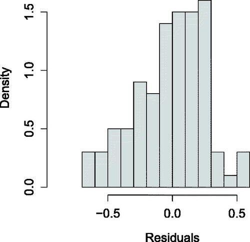It was concluded that ${ϵ}_i\simeq Y_i-4.034-0.045Z_i, i\ge 1$ (see Table S1 in the supplementary material, for details). Assume we aim to investigate the distribution of ϵ_i based on n = 100 biomarkers’ values, when $\text{MI}=1$. In this case, it was observed that the sample mean and variance were $\overline{ϵ}={\sum }_{i=1}^n{ϵ}_i/n\simeq -0.002$ and ${\sum }_{i=1}^n{({ϵ}_i-\overline{ϵ})}^2/(n-1)\simeq 0.073$, respectively. Figure 2 depicts the histogram based on corresponding values of ${ϵ}_1,\dots ,{ϵ}_{100}$.

Fig. 2 Data-based histogram related to regression residuals ${ϵ}_1,\dots ,{ϵ}_n$.

In order to test for $H_0:$ ν = 0 versus $H_1:$ $\nu \ne 0$, where ν is the median of ϵ’s distribution, we implemented the two-sided $T_o^2$-based test and its modification, the $T_N^2$-based test denoted in Section 3.4, as well as the two-sided Wilcoxon-Mann-Whitney test (W). Although the histogram shown in Figure 2 displays a relatively asymmetric distribution about zero, the $T_o^2$-based test and the W test have demonstrated a p-value $=0.071$ and p-value $=0.326$, respectively. The proposed $T_N^2$-based test has provided p-value $=0.047$. Then, we organized a Bootstrap/Jackknife type study to examine the power performances of the test statistics. The conducted strategy was that a sample with size $n_b<100$ was randomly selected with replacement from the data $\left\{{ϵ}_1,\dots ,{ϵ}_n\right\}$ to be tested for H₀ at a 5% level of significance. This strategy was repeated $10,000$ times to calculate the frequencies of the events {$T_o^2$ rejects H₀}, {W rejects H₀}, and {$T_N^2$ rejects H₀}. The obtained experimental powers of $T_o^2$, W, and $T_N^2$ were: 0.238, 0.106, 0.535, when n_b = 90; 0.198, 0.104, 0.463, when n_b = 80; 0.176, 0.100, 0.415, when n_b = 70, respectively. The experimental power levels of the tests increase as the sample size n_b increases. This study experimentally indicates that the $T_N^2$-based test outperforms the classical procedures in terms of the power properties when evaluating whether the residuals of the association $Y_i=a+b{Z}_i+{ϵ}_i, i\ge 1$, are distributed asymmetrically about zero. That is, the proposed test can be expected to be more sensitive as compared with the known methods to rejecting the null hypothesis $H_0:$ ν = 0 versus $H_1:$ $\nu \ne 0$, in this study.

6 Concluding Remarks

The present article has provided a theoretical framework for evaluating and constructing powerful data-based tests. The contributions in this article have touched on the principles of characterizing most powerful statistical decision-making mechanisms. Proposition 2.2 provides a method for one-to-one mapping the term “most powerful” to the properties of test statistics’ distribution functions via analyzing the behavior of corresponding likelihood ratios. We demonstrated that the derived characterization of MP tests can be associated with a principle of sufficiency. The concepts shown in Section 2 have been applied to improving test procedures by accounting for the relevant ancillary statistics. Applications of the presented theoretical framework have been employed to display efficient modifications of the one-sample t-test, the test for the median, and the test for the center of symmetry, in nonparametric settings. The effectiveness of the proposed nonparametric decision-making procedures in maintaining relatively high power has been confirmed using simulations and a real data example across various scenarios based on samples from relatively skewed distributions. We also note the following remarks. (a) Propositions 2.4 and 3.1 can be applied to different decision-making problems. (b) Effective corrections of the classical t-test can be of theoretical and applied interest. The modification of the t-test as per Section 3.3 involves using the estimation of the third central moment. This moment plays a role in some corrections of the t-test structure for adjusting its null distribution when the underlying data are asymmetric, for example, Chen (1995). Overall, the proposed modification is somewhat different from those that are used to improve control of the TIE rates of t-test type procedures. Thus, in general, basic ingredients of the methods mentioned above can be combined. (c) The scheme presented in Section 3.4 can be easily revised to develop a test for quantiles, by using the observation that $\overline{X}$ and the sample pth quantile, say $X_{(pn)}$, are asymptotically bivariate normal with $$\begin{array}{c}\text{cov}\left(\overline{X},X_{(pn)}\right) = f{\left({\nu }_p\right)}^{-1}\mathrm{E}\left(X_1-{\nu }_p\right)\{pI\left(X_1>{\nu }_p\right)\\ \hspace{1em}-(1-p)I\left(X_1\le {\nu }_p\right)\},\\ \text{var}\left(X_{(pn)}\right) = f{\left({\nu }_p\right)}^{-2}p(1-p), \text{Pr}\left(X_1<{\nu }_p\right) = p.\end{array}$$

(d) Sections 3–5 have exemplified applications of the treated MP principle in the nonparametric settings. In many parametric problems, the corresponding likelihood ratios do not have explicit forms or have very complicated shapes, for example, when testing statements are based on longitudinal data, dependent observations, multivariate outcomes, data subject to different sorts of errors, and/or missing-values mechanisms. In such cases, issues related to comparing/developing tests via the considered MP principle can be employed.

A plethora of decision-making algorithms touches on most fields of statistical practice. Thus, it is not practical in one paper to focus on all the relevant theory and examples. This paper studies only one approach to characterize a class of MP mechanisms. That is, there are many potential future directions that seem to be promising targets for research, including, for example: (i) examinations of the relationships between general MP characterizations, Basu’s theorem-type results (e.g., Ghosh 2002), the concepts of sufficiency, completeness, and ancillarity under different statements of decision-making policies. In this aspect, for example, a research question can be as follows: when can we claim that a statistic T is MP iff T and A are independently distributed, for any ancillary statistic A? (ii) Various parametric and nonparametric applications of MP characterizations in different settings can be developed. (iii) Proposition 2.4 can be used and extended to compare different statistical procedures in practice. (iv) In light of the present MP principle, relevant evaluations of optimal combinations of test statistics (e.g., Berk and Jones 1978) can be proposed. (v) Large sample properties of test statistics modified with respect to MP characterization can be analyzed. (vi) Perhaps, Proposition 3.1 can be integrated into various testing developments, where characterizations of underlying data distributions under corresponding hypotheses can be used to define relevant ancillary statistics. Leaving these topics to the future, it is hoped that the present paper will convince the readers of the benefits of studying different aspects and characterizations related to MP data-based decision-making techniques.

Supplementary Materials

The supplementary materials contain: the proofs of the theoretical results presented in the article; and Table S1 that displays the analysis of variance related to the linear regression fitted to the observed log-transformed HDL-cholesterol measurements using the log-transformed TBARS measurements as a factor, in Section 5.

Acknowledgments

The authors are grateful to the Editor, Associate Editor, and an anonymous referee for suggestions that led to a substantial extension and improvement of the presented results.

Additional information

Funding

This work was supported by a National Cancer Institute (NCI) Cancer Center Support Grant (CCSG) to Roswell Park Comprehensive Cancer Center (grant no. P30CA016056). The second author’s research is supported by the following three NCI grants: NRG Oncology Statistical and Data Management Center grant (grant no. U10CA180822); Immuno-Oncology Translational Network (IOTN) Moonshot grant (grant no. U24CA232979-01); Acquired Resistance to Therapy Network (ARTN) grant (grant no.U24CA274159-01).

References

- Bahadur, R. R. (1955), “A Characterization of Sufficiency,” Annals of Mathematical Statistics, 26, 286–293. DOI: 10.1214/aoms/1177728545.
- Bayarri, M. J., and Berger, J. O. (2000), “P Values for Composite Null Models,” Journal of the American Statistical Association, 95, 1127–1142. DOI: 10.2307/2669749.
- Berk, R. H., and Jones, D. H. (1978), “Relatively Optimal Combinations of Test Statistics,” Scandinavian Journal of Statistics, 5, 158–162.
- Bickel, P. J., and Lehmann, E. L. (2012), “Descriptive Statistics for Nonparametric Models I. Introduction,” in Selected Works of EL Lehmann, ed. J. Rojo, pp. 465–471, New York: Springer.
- Boos, D. D., and Hughes-Oliver, J. M. (1998), “Applications of Basu’s Theorem,” The American Statistician, 52, 218–221. DOI: 10.2307/2685927.
- Chen, L. (1995), “Testing the Mean of Skewed Distributions,” Journal of the American Statistical Association, 90, 767–772. DOI: 10.1080/01621459.1995.10476571.
- Efron, B. (1992), Bootstrap Methods: Another Look at the Jackknife, New York: Springer.
- Ferguson, T. S. (1998), “Asymptotic Joint Distribution of Sample Mean and a Sample Quantile,” Unpublished. Available at http://www.math.ucla.edu/∼tom/papers/unpublished/meanmed.pdf.
- Fisher, T. J., and Robbins, M. W. (2019), “A Cheap Trick to Improve the Power of a Conservative Hypothesis Test,” The American Statistician, 73, 232–242. DOI: 10.1080/00031305.2017.1395364.
- Ghosh, I., Balakrishnan, N., and Ng, H. K. T. (2021), Advances in Statistics-Theory and Applications: Honoring the Contributions of Barry C. Arnold in Statistical Science, New York: Springer.
- Ghosh, M. (2002), “Basu’s Theorem with Applications: A Personalistic Review,” Sankhyā: The Indian Journal of Statistics, 64, 509–531.
- Ghosh, M., Reid, N., and Fraser, D. A. S. (2010), “Ancilllary Statistics: A Review,” Statistica Sinica, 20, 1309–1332.
- Hall, P., and La Scala, B. (1990), “Methodology and Algorithms of Empirical Likelihood,” International Statistical Review/Revue Internationale de Statistique, 58, 109–127. DOI: 10.2307/1403462.
- Johnson, V. E. (2013), “Uniformly Most Powerful Bayesian Tests,” The Annals of Statistics, 41, 1716–1741. DOI: 10.1214/13-AOS1123.
- Kagan, A., and Shepp, L. A. (2005), “A Sufficiency Paradox: An Insufficient Statistic Preserving the Fisher Information,” The American Statistician, 59, 54–56. DOI: 10.1198/000313005X21041.
- Lehmann, E. L. (1950), “Some Principles of the Theory of Testing Hypotheses,” The Annals of Mathematical Statistics, 21, 1–26. DOI: 10.1214/aoms/1177729884.
- Lehmann, E. L. (1993), “The Fisher, Neyman-Pearson Theories of Testing Hypotheses: One Theory or Two?” Journal of the American Statistical Association, 88, 1242–1249.
- Lehmann, E. L., and Romano, J. P. (2005), Testing Statistical Hypotheses, New York: Springer.
- Maity, A., and Sherman, M. (2006), “The Two-Sample t test with One Variance Unknown,” The American Statistician, 60, 163–166. DOI: 10.1198/000313006X108567.
- O’Neill, B. (2014), “Some Useful Moment Results in Sampling Problems,” The American Statistician, 68, 282–296. DOI: 10.1080/00031305.2014.966589.
- R Development Core Team. (2012), R: A Language and Environment for Statistical Computing, Vienna, Austria: R Foundation for Statistical Computing. http://www.R-project.org.
- Schisterman, E. F., Faraggi, D., Browne, R., Freudenheim, J., Dorn, J., Muti, P., Armstrong, D., Reiser, B., and Trevisan, M. (2001), “TBARS and Cardiovascular Disease in a Population-based Sample,” Journal of Cardiovascular Risk, 8, 1–7. DOI: 10.1097/00043798-200108000-00006.
- Semkow, T. M., Freeman, N., Syed, U. F., Haines, D. K., Bari, A., Khan, J. A., Nishikawa, K., Khan, A., Burn, A. J., Li, X., and Chu, L. T. (2019), “Chi-Square Distribution: New Derivations and Environmental Application,” Journal of Applied Mathematics and Physics, 7, 1786–1799. DOI: 10.4236/jamp.2019.78122.
- Vexler, A. (2021), “Valid p-values and Expectations of p-values Revisited,” Annals of the Institute of Statistical Mathematics, 73, 227–248. DOI: 10.1007/s10463-020-00747-2.
- Vexler, A., and Hutson, A. (2018), Statistics in the Health Sciences: Theory, Applications, and Computing, New York: CRC Press.
- Vexler, A., Wu, C., and Yu, K. (2010), “Optimal Hypothesis Testing: From Semi to Fully Bayes Factors,” Metrika, 71, 25–138. DOI: 10.1007/s00184-008-0205-4.