Mapping Life Expectancy Loss in Barcelona in 2020

Abstract

We use a Bayesian spatio-temporal model, first to smooth small-area initial life expectancy estimates in Barcelona for 2020, and second to predict what small-area life expectancy would have been in 2020 in absence of covid-19 using mortality data from 2007 to 2019. This allows us to estimate and map the small-area life expectancy loss, which can be used to assess how the impact of covid-19 varies spatially, and to explore whether that loss relates to underlying factors, such as population density, educational level, or proportion of older individuals living alone. We find that the small-area life expectancy loss for men and for women have similar distributions, and are spatially uncorrelated but positively correlated with population density and among themselves. On average, we estimate that the life expectancy loss in Barcelona in 2020 was of 2.01 years for men, falling back to 2011 levels, and of 2.11 years for women, falling back to 2006 levels.

Keywords:

• Bayesian hierarchical model
• Covid-19
• Life expectancy reduction
• Small-area estimation
• Smoothing
• Spatial analysis

1 Introduction

It is difficult to compare the impact of covid-19 in different locations through covid-19 mortality and case rates, because of differences in the rates of testing and in the ways of reporting cause of death. An alternative way to compare that impact that avoids the need to attribute cause of death is to measure it through excess mortality, (see e.g., Islam et al. 2021a; Woolf et al. 2021), but differences in the age pyramid and in the extent to which covid-19 has affected different age groups in different places make that comparison also imperfect.

A third way of assessing the impact of covid-19 that takes into account both excess deaths as well as age of the deceased is through the effect that excess mortality has on life expectancy loss. Life expectancy loss, like excess mortality, cannot distinguish between primary impact caused by covid-19 itself, and secondary impact caused by the effect that covid-19 has had on the mortality rates for other causes, but it serves the purpose of assessing the overall impact of covid-19 on a population beyond the number of covid-19 deaths.

Many studies explore how covid-19 has affected life expectancy at country or large-area level, (see e.g., Aburto et al. 2022; Andrasfay and Goldman 2021, 2022; Castro et al. 2021; Chan, Cheng, and Martin 2021; Islam et al. 2021b; Yadav, Yadav, and Yadav 2021; Mazzuco and Campostrini 2022; Woolf, Masters, and Aron 2022). These investigations are easy to carry out thanks to the availability of age-specific mortality data at country level, and because the size of country populations allow for fairly precise life expectancy estimation, without the need for smoothing.

These large-area studies usually estimate life expectancy loss through the difference between the life expectancy of the year before the pandemic started and the life expectancy of the year when it started, using life expectancy of the first year as if it was the predicted life expectancy of the second year, disregarding the fact that life expectancy has been steadily increasing in most countries. Instead, here we advocate for estimating life expectancy loss through the difference between the life expectancy predicted for the year when the pandemic started in absence of a pandemic, and its actual life expectancy.

Hence, exploring how life expectancy loss varies at small-area level will require life expectancy estimates and predictions based on small-area single year age-specific mortality data, which is not easily available and leads to life expectancy estimates with large variability. As a consequence, one needs accurate spatio-temporal models that help smooth initial life expectancy estimates, and predict life expectancy under a steady state assumption.

Puig and Ginebra (2022) proposes a Bayesian spatio-temporal model that uses space, time and covariate dependencies together with an area level heterogeneity effect to smooth annual small-area life expectancy estimates. Here, that model is proposed as a tool to predict what small-area life expectancies might have been in absence of covid-19, and its performance is assessed by checking how well it predicts small-area life expectancy in Barcelona in 2019, before covid-19 hit, based on the annual life expectancy estimates from 2007 to 2018. That model is then used to predict what small-area life expectancies might have been in 2020 in absence of covid-19, based on the annual life expectancy estimates from 2007 to 2019. That model is also adapted to smooth the small-area life expectancy estimates for 2020 using only age-specific mortality data from 2020.

The small-area life expectancy loss for 2020 due to covid-19 is then estimated by subtracting smoothed life expectancy estimates from predicted ones. By mapping these life expectancy loss estimates and exploring whether they are related to covariates, one can find whether the impact of covid-19 is related to underlying socio-economic or demographic factors.

The article is organized as follows. Section 2 presents the data and Section 3 presents a spatio-temporal model proposed for smoothing small-area life expectancy estimates, and summarizes how life expectancy varied in Barcelona before 2019. Section 4 explains how that same model can be used to predict small-area life expectancy in absence of a pandemic, and checks its performance when predicting life expectancy in 2019. Section 5 adapts that model first to predict life expectancy in 2020 in absence of covid-19, and then to smooth initial life expectancy estimates for 2020. That allows one to map small-area life expectancy loss for 2020 in Barcelona, and explore whether that loss relates to underlying factors.

2 Description of the Data

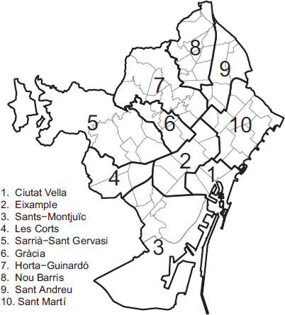
Barcelona, the capital of Catalonia with a population of 792,107 males and of 874,423 females in 2020, is divided into 10 districts and 73 neighborhoods nested in them, as shown in Figure 1. Neighborhoods are very heterogeneous in size, with populations ranging from the least populated neighborhood having only 365 males and 344 females, to the most populated neighborhood having 27,229 males and 31,392 females.

Figure 1: Map of Barcelona divided into 73 neighborhoods nested in 10 districts.

The total number of deaths in 2018 and 2019 in Barcelona were of 7161 and 6995 males, and of 8077 and 7673 females, respectively, while in 2020 the number of deaths increased to 8863 males and 10,105 females.

To obtain the initial small-area annual life expectancy estimates, we used the methodology in Chiang (1968), based on the annual number of deaths and the population by sex, at one year intervals of age, starting from 0 years and up to 89, and aggregating deaths and population at 90 or older. Data was provided by the Department of Statistics of the Oficina Municipal de Dades of the Ajuntament de Barcelona.

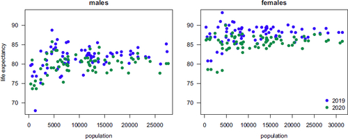
Figure 2 compares the small-area initial life expectancy estimates for 2019 and 2020 as a function of population. Note that the estimates for 2020 tend to be smaller, and that the larger and smaller life expectancy estimates correspond to the smaller areas, due to the larger variability of these estimates. A quarter of the neighborhoods have less than 5000 men and 5000 women, which means that the variability of their initial life expectancy estimates is far too large for these estimates to be of any use by themselves.

Figure 2: Small-area male and female initial life expectancy estimates for 2019 and 2020 as a function of neighborhood population.

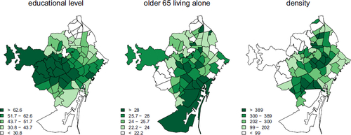
The socio-economic covariates considered to help smooth and predict small-area life expectancy are a household income index, the unemployment rate and the educational level measured through the proportion of individuals with a university or a high school degree. Among demographic covariates, we consider the population density and the proportion of individuals older than 65 living alone. These covariates are intended to capture their effect and as a proxy for variables that are not available. Figure 3 displays the maps of the values of the covariates used in the models. Note that there are strong spatial patterns in them.

Figure 3: Maps of the covariates actually used in the models.

3 Small-Area Life Expectancy Smoothing

In absence of any demographic catastrophe, the initial life expectancy estimates can be smoothed using the model proposed in Puig and Ginebra (2022) for that purpose. The model assumes that the initial annual small-area life expectancy estimates for males (females) in area i and year t, $y_{it}$, are normally distributed. The expected value of $y_{it}$ is split into a constant term, three components capturing covariates, space, and time dependencies, and one component capturing the ith area effect not captured by the other components,(3.1) $$\mathrm{E}(y_{it}|\beta ,{\gamma }_i,{\delta }_0,{\delta }_i,{\alpha }_i)={\beta }_0+\sum _{j=1}^p{\beta }_j{x}_{ji}+{\gamma }_i+({\delta }_0+{\delta }_i)t+{\alpha }_i,$$(3.1) for $i=1,\dots ,n$ and $t=1,\dots ,T$. The covariates effect, ${\beta }_j$, the mean time slope, ${\delta }_0$, and ${\beta }_0$ are considered to be fixed effects. The area effect on the time slope, ${\delta }_i$, and the heterogeneity effect, ${\alpha }_i$, are considered to be random effects with Normal $(0,{\sigma }_{\delta }^2)$ and Normal $(0,{\sigma }_{\alpha }^2)$ distributions, while the spatial effect, ${\gamma }_i$, is considered to be a random effect distributed Normal $(\sum _{k\in v(i)}{\gamma }_k/m_i,{\sigma }_{\gamma }^2/m_i)$, where $v(i)$ is the set of areas neighboring the ith area, and $m_i$ is the number of areas in $v(i)$. The variance of $y_{it}$ is assumed to be inversely proportional to the population, $p_{it}$, of males (females) in that area that year, var $(y_{it}|\beta ,{\gamma }_i,{\delta }_0,{\delta }_i,{\alpha }_i,{\sigma }^2)={\sigma }^2/p_{it}$.

As a prior distribution for ${\beta }_1,\dots ,{\beta }_p$ we choose independent Normal $(0,100)$ distributions. A variance of 100 is large because the covariates are centered and standardized. For ${\beta }_0$ and ${\delta }_0$ we choose independent Normal $(80,100)$ and Normal $(0,100)$ distributions. Finally, for ${\sigma }_{\gamma }^2$, ${\sigma }_{\alpha }^2$, ${\sigma }_{\delta }^2$, and ${\sigma }^2$, we assume that their inverses are Gamma distributed with mean 1 and variance 100. For an alternative modeling approach that first smooths age specific mortality rates, and then uses them to obtain smoothed life expectancy estimates, see Congdon (2009, 2014) or Rashis et al. (2021).

In our applications the model is updated using the MCMC implementation in WinBugs (see Lunn et al. 2000). In them we run four chains until they converge, keeping each one out of 10 simulated values afterwards. The analysis are based on 80,000 draws, 20,000 from each chain. The posterior expected value of $E(y_{it}|\beta ,{\gamma }_i,{\delta }_0,{\delta }_i,{\alpha }_i)$ is used as the smoothed life expectancy estimate for area i and year t.

Figure 4 presents the 2007, 2012, and 2018 life expectancy maps for Barcelona obtained in this way with data from 2007 to 2018. The $95\%$ posterior credible intervals for the coefficients of educational level are $(1.11,1.74)$ for males and $(0.38,0.78)$ for females, the ones for the coefficients of the proportion of older than 65 living alone are $(-1.17,-0.61)$ and $(-0.55,-0.17)$, and the ones for density are $(0.32,0.83)$ and $(0.26,0.61)$, respectively. Income and unemployment were not used because they are correlated with education and do not add anything new to the model.

Figure 4: Maps of the smoothed life expectancy estimates for 2007, 2012, and 2018 categorized in five classes through their time specific quintiles, obtained by updating the full model (3.1) with data from 2007 to 2018.

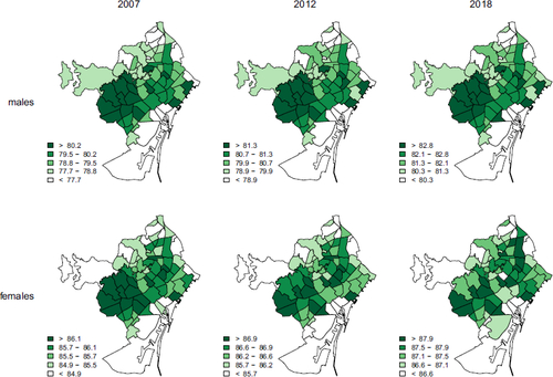
According to Figure 4, before 2019 male life expectancy had a strong persistent spatial dependency, while female life expectancy was becoming less spatially dependent with time. The neighborhoods with the largest life expectancies, in districts 4 and 5, are the wealthier and more educated. Note also that small-area male life expectancies were more variable than female life expectancies. During that period, male life expectancy increased by 0.23 years per year, while female life expectancy increased only by 0.15 years per year, and as a consequence the gap between male and female life expectancy had been steadily decreasing.

4 Small-Area Life Expectancy Prediction

To estimate the life expectancy loss due to covid-19, one needs to predict what that life expectancy would have been in absence of covid-19. A natural way to do that is through the posterior predictive distribution of the full model in Section 3, or of one of the fifteen sub-models obtained by dropping some of the four components of that model. One can actually select the best sub-model of (3.1) for any given application, either based on a model selection criterion, as in Section 5.2, or based on their performance when predicting small-area life expectancy before covid-19 started, the way done here.

To decide which one of these 16 models should be used for prediction in 2020 and to compare the quality of their predictions, these models are used to predict the small-area life expectancies in 2019 using the initial small-area annual life expectancies from 2007 to 2018 to update them. Covid-19 reached Barcelona early in 2020, and so a model will be adequate only if it provides good predictions for 2019.

Table 1 presents the corresponding cross-validated weighted mean square errors of these predictions for 2019, using population of males (females) as weights, together with the Moran Index of residuals indicating that, other than for the baseline model without any of the four components, residuals are close to being spatially independent.

Table 1: Cross-validated weighted mean squared error when predicting life expectancies in 2019 with data from 2007 to 2018, and Moran Index of the residuals.

Covar.	Spat., ${\gamma }_i$	Heter., ${\alpha }_i$	Temp., $({\delta }_0+{\delta }_i)t$	MSE Male	MSE Fem.	MI Male	MI Fem.
No	No	No	No	6.40	4.09	0.224	0.096
Yes	No	No	No	4.99	3.65	–0.011	0.026
No	Yes	No	No	4.25	3.61	0.000	–0.017
No	No	Yes	No	4.24	3.57	0.010	0.012
No	No	No	Yes	2.45	1.84	–0.051	–0.059
Yes	Yes	No	No	4.52	3.55	–0.025	–0.016
Yes	No	Yes	No	4.45	3.54	–0.017	–0.001
Yes	No	No	Yes	2.10	1.82	–0.094	–0.067
No	Yes	Yes	No	4.25	3.60	0.000	–0.014
No	Yes	No	Yes	1.99	1.75	–0.079	–0.059
No	No	Yes	Yes	1.99	1.75	–0.081	–0.052
Yes	Yes	Yes	No	4.49	3.54	–0.024	–0.008
Yes	Yes	No	Yes	2.09	1.79	–0.092	–0.065
Yes	No	Yes	Yes	2.05	1.78	–0.094	–0.063
No	Yes	Yes	Yes	1.99	1.75	–0.080	–0.058
Yes	Yes	Yes	Yes	2.07	1.78	–0.093	–0.063

NOTE: Covariates are educational level, proportion of older than 65 living alone and density.

Each one of the four components separately clearly improve on the predictions obtained with the baseline model. The temporal component is the most useful one, and among all the models with the temporal component, the two models that miss both the spatial and the heterogeneity component are the ones that perform worse, but having both of these components at once does not improve predictions. Among the models that have temporal and either space or heterogeneity components, the ones without covariates perform best.

Hence, prediction in 2020 will be made with the model that only has the temporal and the heterogeneity components, which is the one with the smallest mean square error for the prediction of both the male and the female 2019 life expectancies.

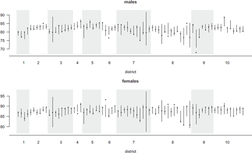
Figure 5 presents the initial life expectancy estimates for 2019, $y_{it}$, together with their $80\%$ posterior predictive intervals for $y_{it}$ under this model. Actual initial male life expectancies fall outside these predictive intervals in 13 out of the 73 neighborhoods, and the female ones fall outside in 15 out of 73 of them, which represents about $18\%$ and $21\%$ of the instances.

Figure 5: Dots are the neighborhood initial life expectancy estimates for 2019 and segments are the $80\%$ posterior predictive intervals, obtained updating model (5.1) with the initial life expectancy estimates from 2007 to 2018.

5 Life Expectancy Loss Estimates for 2020

5.1 Life Expectancy Prediction for 2020 in Absence of Covid-19

A quick and dirty approach to estimate life expectancy loss in 2020 would subtract the life expectancy in 2020 from the one in 2019. This usually under-estimates the loss because in most developed countries life expectancy has been increasing with time.

Instead of that, here the life expectancies that would have been observed in 2020 in absence of covid-19 will be estimated through the posterior predictive distribution of the sub-model of (3.1) with only temporal and heterogeneity components, where:(5.1) $$\mathrm{E}(y_{it}|\beta ,{\gamma }_i,{\delta }_0,{\delta }_i,{\alpha }_i)={\beta }_0+({\delta }_0+{\delta }_i)t+{\alpha }_i,$$(5.1) which is the model that performed best predicting life expectancies in 2019. To update that model, here we use the initial annual life expectancy estimates from 2007 to 2019.

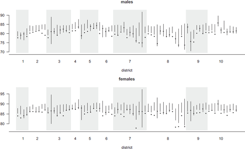
Figure 6 presents the initial life expectancy estimates for 2020 together with the $80\%$ posterior predictive intervals. Male life expectancies fall outside and below these posterior predictive intervals in 36 of the 73 neighborhoods, while the female ones fall outside and below in 44 of them. None of these estimates fall outside and above the corresponding intervals. That is consistent with the observed life expectancy being smaller than predicted in absence of covid-19, and it is in dire contrast with what was found for 2019 in Figure 5. As a predictive estimate of the life expectancy in 2020 in absence of covid-19, we use the expected value of this posterior predictive distribution.

Figure 6: Dots are the neighborhood initial life expectancy estimates for 2020 and segments are the $80\%$ posterior predictive intervals, obtained updating model (5.1) with the initial life expectancy estimates from 2007 to 2019.

5.2 Life Expectancy Smoothing for 2020

Because of covid-19, the effect of the four components of the model for small-area life expectancy, in (3.1), change in 2020, and so when smoothing initial life expectancy estimates for 2020 one can only use the data from 2020, and not the data from previous years.

As a consequence of using only data from a single year, here the model cannot include the temporal component. As a consequence of using only a single observation for each area, the model cannot include the heterogeneity component either, because one cannot estimate the heterogeneity component apart from the spatial and noise components.

Table 2 presents the DIC of the models for 2020 including only the space and/or the covariate component. For male life expectancies, the smallest DIC is attained by the model with both components while for female life expectancies the DIC for that model is close to being the smallest. Hence, the model, with:(5.2) $$\mathrm{E}(y_{it}|\beta ,{\gamma }_i,{\delta }_0,{\delta }_i,{\alpha }_i)={\beta }_0+\sum _{j=1}^p{\beta }_j{x}_{ji}+{\gamma }_i,$$(5.2) will be used to smooth male and female initial life expectancy estimates for 2020.

Table 2: DIC and Moran Index of the residuals when models with covariates and/or spatial component are updated with life expectancy estimates of 2020.

Covar.	Spat., ${\gamma }_i$	DIC Male	DIC Fem.	MI Male	MI Fem.
No	No	319.1	279.4	0.238	0.131
Yes	No	293.7	269.2	0.056	0.014
No	Yes	300.7	278.0	–0.036	0.055
Yes	Yes	289.8	269.7	–0.010	–0.004

NOTE: Covariates are educational level, proportion of older than 65 living alone and density.

The $95\%$ posterior credible intervals for the coefficients of education are $(0.65,1.64)$ for males and $(0.16,0.91)$ for females, the ones for the coefficients of the proportion of older than 65 living alone are $(-1.04,-0.15)$ and $(-0.85,0.12)$, and the ones for density are $(-0.21,0.65)$ and $(0.00,0.71)$, respectively. These intervals are similar to the ones found with the full model and pre-covid-19 mortality data, in Section 3. Note that these coefficients capture the possible effect of these covariates on life expectancy, together with the effect of variables not in the model that are related both with these covariates as well as with life expectancy.

5.3 Life Expectancy Loss for 2020

Neighborhood level life expectancy losses in 2020 are estimated by subtracting their smoothed life expectancy estimates from their predicted life expectancy in absence of covid-19. The overall life expectancy loss in Barcelona can then be estimated through the weighted average of these neighborhood level loss estimates, using male and female population as weights.

Figure 7 presents these life expectancy loss estimates, together with their $80\%$ credibility intervals. Male life expectancy losses are positive in all except seven neighborhoods, and female losses are positive in all of them. The quartiles of these loss estimates are 1.53, 1.93, and 2.58 years in the male case and 1.61, 2.27, and 2.57 years in the female case, with the largest life expectancy losses being 4.76 years for males and of 3.85 years for females. Hence, the distributions of the male and female life expectancy losses are similar. The correlation between male and female life expectancy loss is 0.599.

Figure 7: Dots are the neighborhood life expectancy loss estimates for 2020, and segments are the $80\%$ credible interval for them, using model (5.1) for prediction and model (5.2) for smoothing.

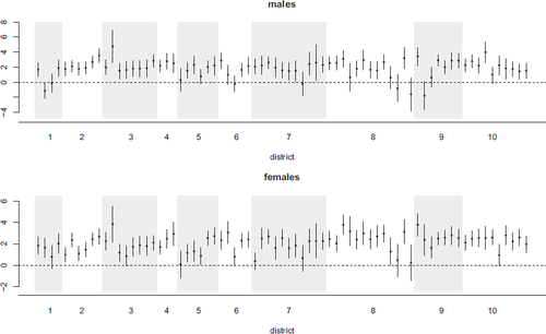
The weighted average of these life expectancy losses is of 2.01 years for males, and of 2.11 years for females. Before 2020, life expectancy in Barcelona was growing by about 0.23 years per year for males and 0.15 years per year for females, and so in 2020 male life expectancy lost what it had gained in the last 8.7 years, falling back to its 2011 level, while female life expectancy lost what it had gained in the last 14.1 years, falling back to its 2006 level.

Aburto et al. (2022) estimates the 2020 life expectancy loss in Spain to be of 1.44 years for males and of 1.50 years for females. Even though these quantities are not completely comparable with the estimates for Barcelona, because they define life expectancy loss as the 2019 minus the 2020 life expectancies, the loss in Barcelona is larger than the one in Spain even after correcting for the difference in estimation method. On the other hand, the life expectancy loss in Barcelona is a lot smaller than the one estimated for Madrid in Diaz-Olalla et al. (2022), which is of 3.67 years for males and of 2.56 years for females.

The 2020 life expectancy loss estimates for nearby countries, in Aburto et al. (2022), are 1.25 years for males and 1.01 years for females in Italy, 0.83 and 0.69 years in Portugal, 0.67 and 0.60 years in France, and 0.38 and 0.23 years in Germany. In contrast, in countries like Norway or Denmark the life expectancy in 2020 was larger than in 2019 in spite of covid-19, while in the United States males lost 2.23 years of life expectancy and females lost 1.63 years. Different from what is found in all countries in Europe except for Spain, Slovenia, and Estonia, in Barcelona the life expectancy loss for females is found to be larger than the one for males.

Figure 8 maps these male and female life expectancy loss estimates. Their Moran Index is 0.023 in the male case and 0.051 in the female one, which are small enough to indicate that these losses are basically spatially uncorrelated. To investigate whether the impact of covid-19 in Barcelona could be related to underlying factors, we looked for correlations between neighborhood life expectancy losses and neighborhood level covariates like unemployment rate, household income, educational level, population density, proportion of individuals older than 65 living alone and an overall socio-economical index.

Figure 8: Map of the life expectancy loss for 2020.

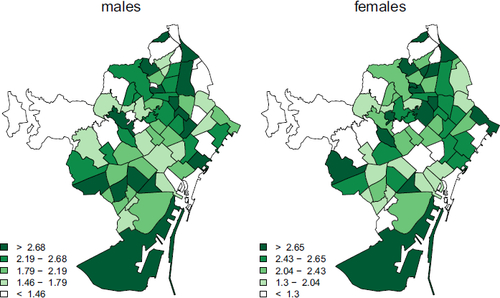
The only significant correlations found were between both male and female life expectancy loss and population density, which were of 0.289 in the case of males and of 0.210 in the case of females. This fact is especially relevant given that Barcelona is one of the most densely populated cities in Europe. Note though that these correlations between the two life expectancy losses and density do not necessarily imply causality, because they capture the combined effect of density together with the effect of other variables related both with density as well as with life expectancy loss, like maybe contamination level, immigrant population rate or household overcrowding.

The fact that no other significant relationships were found, coupled with male and female life expectancy loss estimates turning out to be spatially uncorrelated, seems to indicate that the impact of covid-19 in 2020 was quite even across neighborhoods in Barcelona. The three months that citizens in Barcelona spent under strict home confinement during the first covid-19 wave, coupled with the fact that most of the people living there have universal health coverage, might help in explaining these results.

6 Discussion

Catalonia was one of the hardest hit regions in Europe by the first wave of covid-19, despite the fact that it underwent one of longest and most strict home confinement regimes held outside China. The impact of covid-19 in the capital of Catalonia during that first pandemic year was of about two years of life expectancy lost, and that impact was rather homogeneous in space, with a slightly larger impact in neighborhoods more densely populated.

It would be interesting to use this approach to map small-area life expectancy losses elsewhere, across larger and more heterogeneous regions. It is likely that in that case, one would find relationships between life expectancy losses and other underlying socio-economic, demographic or environmental factors, especially if the investigation involved regions that, unlike Barcelona, did not have universal health coverage. Unfortunately small-area age specific mortality rates and covariates are difficult to obtain, in part due to confidentiality issues, and without them one cannot reproduce this analysis.

Studies that estimate life expectancy loss due to covid-19 for large areas, work with initial life expectancy estimates with a small enough variability to avoid the need for smoothing. And since most of these studies treat life expectancy of the first year as if it was the predicted life expectancy of the second year in absence of covid-19, they do not use any space-time model for prediction either. Instead, we advocate for estimating that loss by subtracting predicted and actual life expectancies for the second year, taking advantage of the fact that the same model used to smooth initial small-area life expectancy estimates can also be used to predict them under steady conditions.

One strength of the space-time model used is the flexibility and ease of interpretation that comes with separating the contribution of the space, time, covariates and heterogeneity components. When it comes to smoothing, our model will only be needed when the small-area populations fall below 10,000 people, because above that the initial life expectancy estimates will have small enough variability to be of use by themselves. When it comes to the prediction part of the problem though, one will always need the model.

Finally, note that the approach presented here could also be used to assess the impact of covid-19 on the small-area mortality rates under causes of mortality other than covid-19 itself. In that case, the data would be the number of deaths under each cause at small-area level, and the model would either be binary logistic or log-linear Poisson. The outcome maps would display mortality rate gaps under the causes considered.

Acknowledgments

The authors are thankful to the Departament d’Estadística de l’Oficina Municipal de Dades de l’Ajuntament de Barcelona for providing the data, and the second author is also grateful for the hospitality of the Department of Mathematics and Statistics of the University of Wyoming, where part of this manuscript was written. We are also extremely grateful for all the comments and suggestions made by the Associate Editor and two reviewers, which helped improve this manuscript a lot.

Disclosure Statement

The authors report that there are no competing interests to declare.

Additional information

Funding

This work was supported by the grant PID2021-125380OB-I00 funded by MCIN/AEI/10.13039/501100011033 and by ERDF A way of making Europe.

References

- Aburto, J. M., Scho, J., Kashnitsky, I., Zhang, L., Rahal, C., Missov, T. I., Mills, M. C., Dowd, J. B., and Kashyap, R. (2022), “Quantifying Impacts of the COVID-19 Pandemic through Life-Expectancy Losses: A Population-Level Study of 29 Countries,” International Journal of Epidemiology, 51, 63–74. DOI: 10.1093/ije/dyab207.
- Andrasfay, T., and Goldman, N. (2021), “Reductions in 2020 US Life Expectancy due to COVID-19 and the Disproportionate Impact on the Black and Latino Populations,” Proceedings of the National Academy of Sciences, 118, e2014746118. DOI: 10.1073/pnas.2014746118.
- Andrasfay, T., and Goldman, N. (2022), “Reductions in US Life Expectancy from COVID-19 by Race and Ethnicity: Is 2021 a Repetition of 2020?” medRxiv [Preprint]. DOI: 10.1101/2021.10.17.21265117.
- Castro, M. C., Gurzenda, S., Turra, C. M., Kim, S., Andrasfay, T., and Goldman, N. (2021), “Reduction in Life Expectancy in Brazil after COVID-19,” Nature Medicine, 27, 1629–1635. DOI: 10.1038/s41591-021-01437-z.
- Chan, E. Y. S., Cheng, D., and Martin, J. (2021), “Impact of COVID-19 on Excess Mortality, Life Expectancy, and Years of Life Lost in the United States,” PloS One, 16, e0256835. DOI: 10.1371/journal.pone.0256835.
- Chiang, C. L. (1968), “The Life Table and its Construction,” in Introduction to Stochastic Processes in Biostatistics, pp. 189–214, New York: Wiley.
- Congdon, P. D. (2009), “Life Expectancies for Small Areas: A Bayesian Random Effects Methodology,” International Statistical Review, 77, 222–240. DOI: 10.1111/j.1751-5823.2009.00080.x.
- Congdon, P. D. (2014), “Estimating Life Expectancies for US Small Areas: A Regression Framework,” Journal of Geographical Systems, 16, 1–18. DOI: 10.1007/s10109-013-0177-4.
- Diaz-Olalla, J. M., Valero-Oteo, I., Moreno-Vazquez, S., Blasco-Novalbos, G., del Moral-Luque, J. A., and Haro-Leon, A. (2022), “Caida de la esperanza de vida en distritos de Madrid en 2020: relacion con determinantes sociales,” Gaceta Sanitaria, 36, 309–316. DOI: 10.1016/j.gaceta.2021.07.004.
- Islam, N., Shkolnikov, V. M., Acosta, J., Klimkin, I., Kawachi, I., Irizarry, R. A., Alicandro, G., Khunti, K., Yates, T., Jdanov, D. A., White, M., Lewington, S., Lacey, B., (2021a), “Excess Deaths Associated with Covid-19 Pandemic in 2020: Age and Sex Disaggregated Time Series Analysis in 29 High Income Countries,” BMJ: British Medical Journal, 373, n1137. DOI: 10.1136/bmj.n1137.
- Islam, N., Jdanov, D. A., Shkolnikov, V. M., Khunti, K., Kawachi, I., White, M., Lewington, S., and Lacey, B. (2021b), “Effects of Covid-19 Pandemic on Life Expectancy and Premature Mortality in 2020: Time Series Analysis in 37 Countries,” BMJ: British Medical Journal, 375, e066768. DOI: 10.1136/bmj-2021-066768.
- Lunn, D. J., Thomas, A., Best, N., and Spiegelhalter, D. (2000), “WinBUGS – A Bayesian Modelling Framework: Concepts, Structure and Extensibility,” Statistics and Computing, 10, 325–337. DOI: 10.1023/A:1008929526011.
- Mazzuco, S., and Campostrini, S. (2022), “Life Expectancy Drop in 2020. Estimates based on Human Mortality Database,” PloS One, 17, e0262846. DOI: 10.1371/journal.pone.0262846.
- Puig, X., and Ginebra, J. (2022), “Bayesian Spatiotemporal Model for Life Expectancy Mmapping; Changes in Barcelona from 2007 to 2018,” Geographical Analysis, 54, 839–859. DOI: 10.1111/gean.12299.
- Rashis, T., Bennett, J. E., Paciorek, C. J., Doyle, Y., Pearson-Stuttard, J., Flaxman, S., Fecht, D., Toledano, M. B., Li, G., Daby, H. I., Johnson, E., Davies, B., and Ezzati, M. (2021), “Life Expectancy and Risk of Death in 6791 Communities in England from 2002 to 2019: High-Resolution Spatiotemporal Analysis of Civil Registration Data,” Lancet Public Health, 6, E805–E816. DOI: 10.1016/S2468-2667(21)00205-X.
- Woolf, S. H., Chapman, D. A., Sabo, R. T., and Zimmerman, E. B. (2021), “Excess Deaths From COVID-19 and Other Causes in the US, March 1, 2020, to January 2, 2021,” JAMA, 325, 1786–1789. DOI: 10.1001/jama.2021.5199.
- Woolf, S. H., Masters, R. K., and Aron, L. Y. (2022), “Changes in Life Expectancy between 2019 and 2020 in the US and 21 Peer Countries,” JAMA Netw Open, 5, e227067. DOI: 10.1001/jamanetworkopen.2022.7067.
- Yadav, S., Yadav, P. K., and Yadav, N. (2021), “Impact of COVID-19 on Life Expectancy at Birth in India: A Decomposition Analysis,” BMC Public Health, 21, 1906. DOI: 10.1186/s12889-021-11690-z.