Distribution-Free Location-Scale Regression

Abstract

We introduce a generalized additive model for location, scale, and shape (GAMLSS) next of kin aiming at distribution-free and parsimonious regression modeling for arbitrary outcomes. We replace the strict parametric distribution formulating such a model by a transformation function, which in turn is estimated from data. Doing so not only makes the model distribution-free but also allows to limit the number of linear or smooth model terms to a pair of location-scale predictor functions. We derive the likelihood for continuous, discrete, and randomly censored observations, along with corresponding score functions. A plethora of existing algorithms is leveraged for model estimation, including constrained maximum-likelihood, the original GAMLSS algorithm, and transformation trees. Parameter interpretability in the resulting models is closely connected to model selection. We propose the application of a novel best subset selection procedure to achieve especially simple ways of interpretation. All techniques are motivated and illustrated by a collection of applications from different domains, including crossing and partial proportional hazards, complex count regression, nonlinear ordinal regression, and growth curves. All analyses are reproducible with the help of the tram add-on package to the R system for statistical computing and graphics.

KEYWORDS:

• Additive models
• Conditional distribution function
• Model selection
• Regression trees
• Smoothing
• Transformation models

1 Introduction

Location-scale regression has its roots in two-sample comparisons, where one extends the location model for some distribution function under treatment $F(y-\mu )$ by adding a scale parameter σ to the location shift μ, that is $F((y-\mu )/\sigma )$, in comparison to the distribution function $F(y)$ under no treatment. One of the earliest contributions is Lepage’s test (Lepage 1971), which is essentially a combination of the Wilcoxon and Ansary-Bradley statistics. Generalized additive models for location, scale, and shape (GAMLSS, Rigby and Stasinopoulos 2005; Stasinopoulos and Rigby 2007) can be motivated as a generalization of the two-sample location-scale model to the regression setup, that is, with covariate-dependent location and scale parameters, $\mu (\mathit{x})$ and $\sigma (\mathit{x})$, and also potentially other parameters $\nu (\mathit{x})$ and $\tau (\mathit{x})$ describing skewness and kurtosis. Thus, GAMLSS allow explanatory variables to affect multiple moments of a variety of parametric distributions and can be understood as an early forerunner of “distributional” regression models (Kneib et al. 2023).

For a continuous response variable Y with explanatory variables $\mathit{X}=\mathit{x}$, GAMLSS are characterized by a parametric distribution $\mathcal{D}$ with typically no more than four parameters $\mu (\mathit{x})$ for location, $\sigma (\mathit{x})$ for scale, $\nu (\mathit{x})$ for skewness, and $\tau (\mathit{x})$ for kurtosis. For the simplest case assuming a normal distribution $\mathcal{D}=\mathrm{N}(\mu (\mathit{x}),\sigma {(\mathit{x})}^2)$ for the conditional response of $Y\in \mathbb{R}$, the model can be written in terms of the conditional mean $\mu (\mathit{x})$ and standard deviation $\sigma (\mathit{x})$ as $$\mathbb{P}(Y\le y\mid \mathit{X}=\mathit{x})=\Phi \left(\frac{y-\mu (\mathit{x})}{\sigma (\mathit{x})}\right),$$with $\Phi$ being the standard normal cumulative distribution function. Without relying on such a prior assumption of a parametric distribution $\mathcal{D}$, (Tosteson and Begg 1988,eq. 1) introduced a distribution-free location-scale ordinal regression model in the context of receiver operating characteristic (ROC) analysis for ordinal responses $Y\in \{y_1<y_2<\cdots <y_K\}$ formulated as a conditional cumulative distribution function (1) $$\begin{array}{c}\mathbb{P}(Y\le y_k\mid \mathit{X}=\mathit{x})=F\left(\frac{{\vartheta }_k-\mu (\mathit{x})}{\sigma (\mathit{x})}\right),\\ k=1,\dots ,K-1\end{array}$$(1) with intercept thresholds ${\vartheta }_k$ depending on the kth response category, parameters ${\vartheta }_k\le {\vartheta }_{k+1}$ being monotonically nondecreasing. The model features two model terms, $\mu (\mathit{x})$ and $\sigma (\mathit{x})$, and is defined by a cumulative distribution function F. Tosteson and Begg (1988) discuss normal ($F=\Phi$) and logit models ($F={\text{logit}}^{-1}$) in more detail. The latter corresponds to the “non-linear” odds model discussed in (McCullagh 1980,sec. 6.1), which was later extended in terms of “partial proportional odds models” (Peterson and Harrell 1990). A very attractive feature of such models is their distribution-free nature and easily comprehensible covariate-dependence through location-scale parameters $\mu (\mathit{x})$ and $\sigma (\mathit{x})$. However, they lack the broad applicability of the GAMLSS family, for example to censored, bounded or mixed discrete-continuous responses. Inspired by location-scale ordinal regression our primary aim is to develop a distribution-free and parsimonious flavor of GAMLSS.

We propose a generalization of location-scale ordinal regression by introducing a smooth parsimonious parameterization of the intercept thresholds in terms of a transformation function, allowing to estimate distribution-free location-scale models for continuous, discrete, and potentially censored or truncated outcomes in a unified maximum likelihood framework (Hothorn et al. 2018). This framework of location-scale transformation models allows one to model the impact of explanatory variables on the location and the dispersion of the response distribution, without relying on distributional assumptions. We demonstrate the practical merits of such an approach by applications of (a) maximum-likelihood estimation in stratified models and models for crossing or partially proportional hazards, (b) novel location-scale regression trees, (c) transformation models with smooth nonlinear location-scale parameters for growth-curve analysis, and discuss (d) model selection issues arising in these contexts.

2 Model

For univariate and at least ordered responses variables $Y\in \Xi$ we propose to study regression models describing the conditional distribution function of Y given explanatory variables $\mathit{X}=\mathit{x}$ as (2) $$\begin{array}{c}\mathbb{P}(Y\le y\mid \mathit{X}=\mathit{x})=F\left(\sigma {(\mathit{x})}^{-1}h(y\mid \vartheta )-\mu (\mathit{x})\right),\\ \mathrm{\hspace{1em}}\mathrm{\hspace{1em}}y\in \Xi .\end{array}$$(2)

The model is characterized by (i) a monotonically increasing transformation function $h:\Xi \to \mathbb{R}$ depending on parameters $\vartheta \in {\mathbb{R}}^P$, (ii) a cumulative distribution function $F:\mathbb{R}\to [0,1]$ of some random variable with log-concave Lebesgue density on the real line, (iii) a covariate-dependent location parameter $\mu (\mathit{x})\in \mathbb{R}$, and (iv) a covariate-dependent scale parameter $\sigma (\mathit{x})\in {\mathbb{R}}^{+}$. The model is distribution-free in the sense that a unique transformation function h exists for every baseline distribution $\mathbb{P}(Y\le y\mid \mathit{X}={\mathit{x}}_0)$, that is, a distribution conditional on explanatory variables ${\mathit{x}}_0$ with $\mu ({\mathit{x}}_0)=0$ and $\sigma ({\mathit{x}}_0)=1$. In this case, the transformation function is given by $h(y\mid \vartheta )=F^{-1}(\mathbb{P}(Y\le y\mid \mathit{X}={\mathit{x}}_0))$. Conditional distributions arising from changing ${\mathit{x}}_0$ to $\mathit{x}$ are linear in h on the scale of the link function $F^{-1}(\mathbb{P}(Y\le y\mid \mathit{X}=\mathit{x}))=\sigma {(\mathit{x})}^{-1}h(y\mid \vartheta )-\mu (\mathit{x})$. 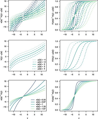Unknowns to be estimated are the parameters $\vartheta$ defining the transformation function, the location function $\mu (\mathit{x})$, and the scale function $\sigma (\mathit{x})$, whereas F is chosen a priori. The applicability to ordered, count, or continuous outcomes possibly under random censoring, its distribution-free nature, and the location-scale formulation allowing simple interpretation of the impact explanatory variables have on the response’ distribution shall be discussed in the following. Figure 1 illustrates the flexibility of the location-scale transformation model on the scale of the link function, that is $F^{-1}(\mathbb{P}(Y\le y\mid \mathit{X}=\mathit{x}))$, and of the conditional distribution function $\mathbb{P}(Y\le y\mid \mathit{X}=\mathit{x})$ for different values of $\mu (\mathit{x})$ and $\sigma (\mathit{x})$.

Fig. 1 Location-scale transformation model. The transformation (left) and cumulative distribution function (right) are shown for the baseline configuration (i.e., $\mu (\mathit{x})=0$ and $\sigma (\mathit{x})=1$) and different values of the location parameter $\mu (\mathit{x})$ and of the scale parameter $\sigma (\mathit{x})$.

2.1 Interpretation

In all models (2), positive values of the location parameter $\mu (\mathit{x})$ correspond to larger values of the response and smaller values of the scale parameter $\sigma (\mathit{x})$ are associated with smaller variability of the response and thus result in more “concentrated” conditional distributions (Figure 1). Fitted models can conveniently be inspected on the scale of the conditional distribution, survival, density, (cumulative) hazard, odds, or quantile functions.

Statements beyond these general facts and interpretation of $\mu (\mathit{x})$ and $\sigma (\mathit{x})$ in particular depend on the specific choice of F. Suitable choices for F include inverses of common link functions, such as $F=\Phi ={\text{probit}}^{-1},F={\text{logit}}^{-1},F={\text{cloglog}}^{-1}$, or $F={\text{loglog}}^{-1}$. For $\sigma (\mathit{x})\equiv 1$, the model reduces to well-established regression models. For $F={\text{cloglog}}^{-1}$, one obtains a proportional hazards model, a proportional reverse-time hazards model is defined by $F={\text{loglog}}^{-1}$, and a proportional odds model given by the choice $F={\text{logit}}^{-1}$. For $F=\Phi$, $\mu (\mathit{x})=\mathbb{E}(h(Y\mid \vartheta )\mid \mathit{x})$ is the conditional mean of the h-transformed response. An overview on these models and interpretation of $\mu (\mathit{x})$ is available from (Hothorn et al. 2018,Table 1).

Under certain circumstances, these simple ways of interpretation carry over to location-scale models of form (2). Consider Cox’ proportional hazards model ($F={\text{cloglog}}^{-1}$) for a continuous survival time. A change from $\mathit{x}$ to $\tilde{\mathit{x}}$ is reflected by the difference $\mu (\tilde{\mathit{x}})-\mu (\mathit{x})$ on the scale of the log-hazard functions conditional on $\mathit{x}$ and $\tilde{\mathit{x}}$, respectively. The introduction of a scale parameter $\sigma (\mathit{x})$ to this model does not affect this form of interpretation as long as $\sigma (\mathit{x})=\sigma (\tilde{\mathit{x}})$, owing to the fact that in model (2) $\mu (\mathit{x})$ is not multiplied with $\sigma {(\mathit{x})}^{-1}$. For a proportional odds model, $\mu (\tilde{\mathit{x}})-\mu (\mathit{x})$ is the vertical difference between the two conditional log-odds functions. Therefore, if model interpretation on these scales is important for certain explanatory variables, one should try to omit these variables from the scale term.

Another form of model interpretation can be motivated from probabilistic index models (Thas et al. 2012), which describe the impact of a transition from $\mathit{x}$ to $\tilde{\mathit{x}}$ by the probabilistic index $\mathbb{P}(Y\le \tilde{Y}\mid \mathit{x},\tilde{\mathit{x}})$. This probability can be derived from transformation models (Sewak and Hothorn 2023). For the probit location-scale transformation model $\Phi (\sigma {(\mathit{x})}^{-1}h(y\mid \vartheta )-\mu (\mathit{x}))$, for example, the probabilistic index has a simple form, $$\begin{array}{c}\mathbb{P}\left(Y\le \tilde{Y}\mid \mathit{x},\tilde{\mathit{x}}\right)=\mathbb{P}\left(h(Y\mid \vartheta )\le h(\tilde{Y}\mid \vartheta )\mid \mathit{x},\tilde{\mathit{x}}\right)\\ =\Phi \left(\frac{\sigma (\tilde{\mathit{x}})\mu (\tilde{\mathit{x}})-\sigma (\mathit{x})\mu (\mathit{x})}{\sqrt{\sigma {(\tilde{\mathit{x}})}^2+\sigma {(\mathit{x})}^2}}\right),\end{array}$$with two independent draws from this model, the first, Y, conditional on $\mathit{x}$ and the second, $\tilde{Y}$, conditional on $\tilde{\mathit{x}}$. Especially in cases where an explanatory variable affects both the location term $\mu (\mathit{x})$ but also the scale term $\sigma (\mathit{x})$, the probabilistic index may serve as a comprehensive measure to describe the impact of changes in the covariate configuration on the response’s distribution.

2.2 Parameterization

We in general express the transformation function in terms of P basis functions $h(y\mid \vartheta )=\mathit{a}{(y)}^{\top }\vartheta$. For absolute continuous responses $Y\in \Xi \subseteq \mathbb{R}$, the transformation function h can be conveniently parameterized in terms of a polynomial in Bernstein form $h(y\mid \vartheta )={\mathit{a}}_{\text{Bs},P-1}{(y)}^{\top }\vartheta$ (McLain and Ghosh 2013; Hothorn et al. 2018). The basis functions ${\mathit{a}}_{\text{Bs},P-1}(y)\in {\mathbb{R}}^P$ are specific beta densities (Farouki 2012) and it is straightforward to obtain derivatives and integrals of $h(y\mid \vartheta )={\mathit{a}}_{\text{Bs},P-1}{(y)}^{\top }\vartheta$ with respect to y and, under suitable constraints, a monotonically increasing transformation function h (Hothorn et al. 2018). For count responses $Y\in \{0,1,2,\dots \}$ this transformation function is evaluated for integer values only, that is, $h(\lfloor y\rfloor \mid \vartheta )$ (Siegfried and Hothorn 2020). For ordered categorical responses $Y\in \{y_1<\cdots <y_K\}$ the transformation function is defined such that $\mathit{a}{(y_k)}^{\top }\vartheta ={\vartheta }_k$ depending on the category $k=1,\dots ,K-1$. A nonparametric version assigns one parameter to each unique value of the outcome in the same way. In all cases, monotonicity of h can be implemented by the constraints ${\vartheta }_p\le {\vartheta }_{p+1},p\in 1,\dots ,P-1$ (Hothorn et al. 2018).

2.3 Likelihood

From model (2), the log-likelihood contribution ${\mathcal{l}}_i(\vartheta ,\mu ({\mathit{x}}_i),\sigma ({\mathit{x}}_i))$ of an observation $(y_i,{\mathit{x}}_i)$ with $y_i\in \mathbb{R}$ given as a function of the unknown parameters $\vartheta ,\mu ({\mathit{x}}_i)$, and $\sigma ({\mathit{x}}_i)$ is (3) $$\begin{array}{c}\hspace{0.17em}\log \hspace{0.17em}\left[f\left\{\sigma {({\mathit{x}}_i)}^{-1}h(y_i\mid \vartheta )-\mu ({\mathit{x}}_i)\right\}\right]\\ \hspace{1em}+\hspace{0.17em}\log \hspace{0.17em}\left[\sigma {({\mathit{x}}_i)}^{-1}\right]+\hspace{0.17em}\log \hspace{0.17em}\left[h\prime (y_i\mid \vartheta )\right].\end{array}$$(3)

Evaluating this expression requires the Lebesgue density $f=F\prime$ and the derivative $h\prime (y\mid \vartheta )=\mathit{a}\prime {(y)}^{\top }\vartheta$ of the transformation function with respect to y. For a discrete, left-, right- or interval-censored observation $(\underset{--}{y_i},{\overline{y}}_i]$ the exact log-likelihood contribution ${\mathcal{l}}_i(\vartheta ,\mu ({\mathit{x}}_i),\sigma ({\mathit{x}}_i))=\hspace{0.17em}\log \hspace{0.17em}\{\mathbb{P}(Y\in (\underset{--}{y_i},{\overline{y}}_i]\mid {\mathit{x}}_i)\}$ is (4) $$\begin{array}{c}\hspace{0.17em}\log \left[F\right\{\sigma {({\mathit{x}}_i)}^{-1}h({\overline{y}}_i\mid \vartheta )-\mu ({\mathit{x}}_i)\}\\ -F\{\sigma {({\mathit{x}}_i)}^{-1}h(\underset{--}{y_i}\mid \vartheta )-\mu ({\mathit{x}}_i)\}].\end{array}$$(4)

For observed categories $y_k$, the datum is specified by $(y_{k-1},y_k]$ and for counts $y_i\in \mathbb{N}$ it is $(\underset{--}{y_i},{\overline{y}}_i]=(y_i-1,y_i]$. For random right-censoring at time t_i it is given by $(\underset{--}{y_i},{\overline{y}}_i]=(t_i,\infty )$ and for left-censoring at time t_i by $(\underset{--}{y_i},{\overline{y}}_i]=(0,t_i]$.

For the important special case of $i=1,\dots ,N$ independent realizations from model (2) with linear location term $\mu (\mathit{x})={\mathit{x}}^{\top }\mathit{\beta }$ and log-linear form for the scale term $\sigma {(\mathit{x})}^{-1}=\sqrt{\hspace{0.17em}\exp \hspace{0.17em}({\mathit{x}}^{\top }\mathit{\gamma })}$, the unknown parameters $\vartheta ,\mathit{\beta }$, and $\mathit{\gamma }$ can be estimated simultaneously by maximizing the corresponding log-likelihood under suitable constraints $$\begin{array}{c}({\widehat{\vartheta }}_N,{\widehat{\mathit{\beta }}}_N,{\widehat{\mathit{\gamma }}}_N)=\text{arg} {\max }_{\vartheta ,\mathit{\beta },\mathit{\gamma }}\sum _{i=1}^N{\mathcal{l}}_i\left(\vartheta ,{\mathit{x}}_i^{\top }\mathit{\beta },{\sqrt{\hspace{0.17em}\exp \hspace{0.17em}({\mathit{x}}_i^{\top }\mathit{\gamma })}}^{-1}\right)\\ \text{subject to }{\vartheta }_p\le {\vartheta }_{p+1},p\in 1,\dots ,P-1.\end{array}$$

Score functions and Hessians as well as conditions for likelihood-based inference can be derived from the expressions given in Hothorn et al. (2018) for models defined in terms of $\vartheta$ and $\mathit{\beta }$.

2.4 Model Selection

Model selection in this framework can be performed by including an L₀ penalty in the likelihood implied by model (2) $$\begin{array}{c}{\max }_{\vartheta \in {\mathbb{R}}^P,\mathit{\beta }\in {\mathbb{R}}^J,\mathit{\gamma }\in {\mathbb{R}}^J}\sum _{i=1}^N{\mathcal{l}}_i\left(\vartheta ,{\mathit{x}}_i^{\top }\mathit{\beta },{\sqrt{\hspace{0.17em}\exp \hspace{0.17em}({\mathit{x}}_i^{\top }\mathit{\gamma })}}^{-1}\right),\\ \text{subject to }{\Vert {\left({\mathit{\beta }}^{\top },{\mathit{\gamma }}^{\top }\right)}^{\top }\Vert }_0\le s,\end{array}$$using an adaptation of the sequencing-and-splicing technique suggested by Zhu et al. (2020). Here, $s\in \{1,\dots ,2J\}$ denotes a fixed support size and ${\Vert ·\Vert }_0$ denotes the L₀ norm. The parameters of the transformation function $\vartheta$ remain unpenalized. When the support size s is unknown, s is tuned by minimizing a high-dimensional information criterion (SIC). The procedure is summarized in Algorithm 1. Further information on the choice of the initial active set and the inclusion of unpenalized parameters is given in the supplementary material C.

Algorithm 1

Best subset selection for location-scale transformation models.

Require: Data ${\{(y_i,{\mathit{x}}_i)\}}_{i=1}^N\in {(\Xi \times {\mathbb{R}}^J)}^N$, max. support size $s_{\max }\in \{1,\dots ,2J\}$, max. splicing size $k_{\max }\le s_{\max }$, tuning threshold ${\tau }_s\in {\mathbb{R}}_{+}$ for $s=1,\dots ,s_{\max }$

1: Fit unconditional model: $\hspace{1em}\widehat{\vartheta }\leftarrow \text{arg} {\max }_{\vartheta \in {\mathbb{R}}^P}{\sum }_{i=1}^N{\mathcal{l}}_i(\vartheta ,0,1)$

2: Compute bivariate score residuals: $${(r_{\text{loc}},r_{\text{sc}})}_i\leftarrow {\frac{\partial }{\partial (\beta ,\gamma )}{\mathcal{l}}_i\left(\vartheta ,\beta ,{\sqrt{\hspace{0.17em}\exp \hspace{0.17em}(\gamma )}}^{-1}\right)|}_{\vartheta =\widehat{\vartheta },\beta =0,\gamma =0}$$

3: for $s=1,2,\dots ,s_{\max }$ do

4: Initialize active set: $$\begin{array}{c}{\mathcal{A}}_s^0=\{i:\sum _{j=1}^{J}1\left(\left|\text{cor}({\mathit{x}}_j,{\mathit{r}}_{\text{loc}})\right|\ge \left|\text{cor}({\mathit{x}}_i,{\mathit{r}}_{\text{loc}})\right|\right)+\\ \sum _{k=J+1}^{2J}1\left(\left|\text{cor}({\mathit{x}}_k,{\mathit{r}}_{\text{sc}})\right|\ge \left|\text{cor}({\mathit{x}}_i,{\mathit{r}}_{\text{sc}})\right|\right)\le s\},\\ {\mathcal{I}}_s^0=\{1,\dots ,2J\}\backslash {\mathcal{A}}_s^0\end{array}$$

5: for $m=0,1,2,\dots$ do

6: Run Algorithm 2 in Zhu et al. (2020): $$\left({\widehat{\vartheta }}_s^{m+1},{\widehat{\mathit{\beta }}}_s^{m+1},{\widehat{\mathit{\gamma }}}_s^{m+1},{\mathcal{A}}_s^{m+1},{\mathcal{I}}_s^{m+1}\right)\leftarrow$$ $$\mathrm{Splicing}({\widehat{\vartheta }}_s^m,{\widehat{\mathit{\beta }}}_s^m,{\widehat{\mathit{\gamma }}}_s^m,{\mathcal{A}}_s^m,{\mathcal{I}}_s^m,k_{\max },{\tau }_s)$$

7: if $({\mathcal{A}}_s^{m+1},{\mathcal{I}}_s^{m+1})=({\mathcal{A}}_s^m,{\mathcal{I}}_s^m)$ then

8: stop

9: end if

10: end for

11: $$\left({\widehat{\vartheta }}_s,{\widehat{\mathit{\beta }}}_s,{\widehat{\mathit{\gamma }}}_s,{\widehat{\mathcal{A}}}_s\right)\leftarrow \left({\widehat{\vartheta }}_s^{m+1},{\widehat{\mathit{\beta }}}_s^{m+1},{\widehat{\mathit{\gamma }}}_s^{m+1},{\mathcal{A}}_s^{m+1}\right)$$

12: end for

13: Choose optimal support size based on SIC: $$\widehat{s}=\text{arg} {\min }_s-\sum _{i=1}^N{\mathcal{l}}_i\left({\widehat{\vartheta }}_s,{\mathit{x}}_i^{\top }{\widehat{\mathit{\beta }}}_s,{\sqrt{\hspace{0.17em}\exp \hspace{0.17em}({\mathit{x}}_i^{\top }{\widehat{\mathit{\gamma }}}_s)}}^{-1}\right)+$$ $${\Vert {\left({\widehat{\mathit{\beta }}}_s^{\top },{\widehat{\mathit{\gamma }}}_s^{\top }\right)}^{\top }\Vert }_0(\hspace{0.17em}\log \hspace{0.17em}2J)(\hspace{0.17em}\log \hspace{0.17em}\hspace{0.17em}\log \hspace{0.17em}N)$$

14: return $({\widehat{\vartheta }}_{\widehat{s}},{\widehat{\mathit{\beta }}}_{\widehat{s}},{\widehat{\mathit{\gamma }}}_{\widehat{s}},{\widehat{\mathcal{A}}}_{\widehat{s}})$

3 Inference for Applications

Motivated by applications from different domains we detail the estimation of location-scale transformation models, including important aspects of model evaluation, interpretation and testing. The wide range of applications of the model framework is further exemplified by contrasting it to established location-scale models.

In Section 3.1.1 we outline the estimation of location-scale transformation models from the perspective of a stratified model. Section 3.1.2 presents the application of location-scale models to survival data in the presence of crossing hazards, further introducing a location-scale alternative to the commonly used log-rank test. Interpretability of location-scale transformation models is exemplified in Section 3.1.3 assessing seasonal and annual patterns of deer-vehicle collisions. The estimation of nonlinear, tree-based location-scale transformation models is discussed for self-reported orgasm frequencies of Chinese women in Section 3.2. Inspired by the GAMLSS framework, Section 3.3 describes the estimation of a distribution-free version of additive models featuring smooth covariate-dependent location and scale terms. The application of model selection in this framework is exemplified in Section 3.4.

All analyses can be replicated using the tram R package (Hothorn et al. 2023) with $$\mathrm{R}\mathrm{>}\text{ demo}\left(\mathrm{"}\text{stram}\mathrm{"}\text{, package = }\mathrm{"}\text{tram}\mathrm{"}\right)$$

3.1 Maximum Likelihood

3.1.1 Stratification

Haslinger et al. (2020) reported data from measuring postpartum blood loss $Y\in {\mathbb{R}}^{+}$ during 676 vaginal deliveries and 632 caesarean sections at the University Hospital Zurich, Switzerland. Aiming to contrast blood loss during vaginal deliveries or cesarean sections the conditional distributions can be estimated by stratification, for example.

In the following we estimate such a stratified model with two separate transformation functions $h(y\mid \text{delivery}=\text{vaginal})={\mathit{a}}_{\text{Bs},15}{(y)}^{\top }{\vartheta }_{\text{vaginal}}$ and $h(y\mid \text{delivery}=\text{cesarean})={\mathit{a}}_{\text{Bs},15}{(y)}^{\top }{\vartheta }_{\text{cesarean}}$ as polynomials in Bernstein form. In a similar spirit, a location-scale transformation model with transformation function ${\mathit{a}}_{\text{Bs},15}{(y)}^{\top }\vartheta$ for vaginal deliveries and transformation function $\sqrt{\hspace{0.17em}\exp \hspace{0.17em}(\gamma )}{\mathit{a}}_{\text{Bs},15}{(y)}^{\top }\vartheta -\beta$ for cesarean sections can be defined. Transformation functions of both models were defined on the probit scale. The stratified, distribution- and model-free approach estimates $2\times P=32$ parameters whereas the distribution-free location-scale model consists of only $P+2=18$ parameters, providing a lower-dimensional alternative to stratification. Owing to Weierstrass’ theorem, polynomials in Bernstein form with sufficiently large order $P-1$ can approximate any continuous function on an interval and therefore the location-scale model does not make assumptions about the transformation function h and thus the distribution of blood loss for vaginal deliveries. However, the location and scale terms govern the discrepancy between blood loss distributions for the two modes of delivery, and thus this approach can be characterized as being distribution-free but not model-free.

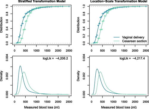
Due to the practical challenges in measuring blood loss in the hectic environment of a delivery ward, interval-censored observations were reported and the corresponding interval-censored negative log-likelihood (4) is minimized by Augmented Lagrangian Minimization (Madsen et al. 2004) to estimate the parameters $\vartheta ,\beta$, and $\gamma$ simultaneously. Visual inspection of distribution and density functions as well as the in-sample log-likelihoods in Figure 2 shows that the two models are practically identical. The two estimated conditional distribution functions cross around 1000 ml, which is only possible due to estimation of two separate transformation functions $h(y\mid \text{delivery})$ or via the inclusion of the delivery mode dependent scale term $\sqrt{\hspace{0.17em}\exp \hspace{0.17em}(\gamma )}$.

Fig. 2 Stratification. Distribution (top) and density (bottom) of postpartum blood loss conditional on delivery mode estimated by the stratified transformation model (left) and location-scale transformation model (right). In addition, the empirical cumulative distribution function is shown in the top row, in-sample log-likelihoods are given in the bottom row.

We can also compute the probabilistic index here, which indicates that a randomly selected woman having a vaginal delivery has a probability of 0.71 (95% confidence interval: 0.68–0.74) for a lower blood loss compared to a randomly selected woman undergoing a cesarean section.

3.1.2 Crossing Hazards

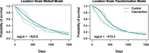
In the following we reanalyze a two-arm randomized controlled trial of 90 patients with gastric cancer (Schein and Gastrointestinal Tumor Study Group 1982). Trial patients received either chemotherapy and radiotherapy (intervention group) or chemotherapy alone (control group). The nonparametric Kaplan-Meier estimates of the survivor functions of both groups in Figure 3 reveal crossing of the curves at approximately 1000 days, and thus nonproportional hazards.

Fig. 3 Crossing hazards. The survivor functions of the two groups estimated by the nonparametric Kaplan-Meier method (step function) are shown along the estimates from the location-scale Weibull model (left) and the distribution-free location-scale transformation model (right).

Nonproportional hazards are a common violation of a standard model assumption in survival analysis necessitating tailored models to express differences in survival times $T\in {\mathbb{R}}^{+}$ by interpretable parameters. We suggest a location-scale transformation model of the form $$\mathbb{P}(T>t\mid \text{control})=\hspace{0.17em}\exp [-\hspace{0.17em}\exp \hspace{0.17em}\{h(t\mid \vartheta )\left\}\right]$$ $$\mathbb{P}(T>t\mid \text{intervention})=\hspace{0.17em}\exp \hspace{0.17em}\left[-\hspace{0.17em}\exp \hspace{0.17em}\left\{\sqrt{\hspace{0.17em}\exp \hspace{0.17em}(\gamma )}h(t\mid \vartheta )-\beta \right\}\right].$$

For $\gamma =0$, the model reduces to a proportional hazards model with log-hazard ratio $\beta$. A distribution-free version can be implemented by choosing a polynomial in Bernstein form for the transformation function $h(t\mid \vartheta )={\mathit{a}}_{\text{Bs},6}{(t)}^{\top }\vartheta$. A Weibull model corresponds to a log-linear transformation function $h(t\mid \vartheta )={\vartheta }_1+{\vartheta }_2\hspace{0.17em}\log \hspace{0.17em}(t)$, which was introduced as a special case in the GAMLSS framework (Rigby and Stasinopoulos 2005,Table 1) and later investigated in more detail by Burke and MacKenzie (2017) and Peng et al. (2020) using the equivalent parameterization ${\vartheta }_1+\hspace{0.17em}\exp \hspace{0.17em}({\vartheta }_2)\hspace{0.17em}\log \hspace{0.17em}(t)$ for the control and ${\vartheta }_1+\hspace{0.17em}\exp \hspace{0.17em}({\vartheta }_2+\gamma )\hspace{0.17em}\log \hspace{0.17em}(t)+\beta$ for the intervention group. Further extensions of the Weibull location-scale model were studied in Burke et al. (2020b) and a nonparametric approach, leaving h completely unspecified, was theoretically discussed by Zeng and Lin (2007) and Burke et al. (2020a).

Model parameters for both models were estimated by maximizing the likelihood defined by (3) for death times and likelihood (4) for right-censored observations. The nonparametric Kaplan-Meier estimates in Figure 3 are overlaid with survivor functions obtained from the Weibull model (log-linear h, left panel) and the distribution-free location-scale model (h being a polynomial in Bernstein form, right panel). Both models show crossing survivor curves and the more flexible model appears to have better fit. However, in the context of a randomized trial, a test for the null hypothesis of equal survivor curves is more important than model fit. The likelihood ratio tests lead to a rejection of the null at 5% in either model (p-value $=0.034$ for the Weibull model and p-value $=0.011$ for the distribution-free model). The bivariate Wald-test, proposed by Burke and MacKenzie (2017) for crossing-hazards problems, also leads to a rejection with p-value $=0.032$.

An alternative location-scale test can be motivated in analogy to the log-rank test. The bivariate permutation score test for $\gamma$ and $\beta$ for testing the null $\gamma =\beta =0$ is defined based on the unconditional model $\mathbb{P}(T>t)=\hspace{0.17em}\exp [-\hspace{0.17em}\exp \hspace{0.17em}\{h(t\mid \vartheta )\}]$, that is, the model fitted under the constraint $\gamma =\beta =0$. Thus, the likelihood contribution of the ith subject is ${\mathcal{l}}_i(\vartheta ,\beta ,{\sqrt{\hspace{0.17em}\exp \hspace{0.17em}(\gamma )}}^{-1})={\mathcal{l}}_i(\vartheta ,0,1)$. The maximum-likelihood estimator is $$\begin{array}{c}\widehat{\vartheta }=\text{arg} {\max }_{\vartheta }\sum _{i=1}^N{\mathcal{l}}_i(\vartheta ,0,1),\\ \mathrm{\hspace{1em}}\mathrm{\hspace{1em}}\text{subject to }\hspace{1em}{\vartheta }_p\le {\vartheta }_{p+1},p\in 1,\dots ,P-1.\end{array}$$

The individual score contributions are defined as $${\mathit{r}}_i={\frac{\partial {\mathcal{l}}_i\left(\vartheta ,\beta ,{\sqrt{\hspace{0.17em}\exp \hspace{0.17em}(\gamma )}}^{-1}\right)}{\partial (\beta ,\gamma )}|}_{\vartheta =\widehat{\vartheta },\beta =0,\gamma =0}\in {\mathbb{R}}^2.$$

Note that the first element of ${\mathit{r}}_i$ is the log-rank score for the ith individual and a bivariate linear test statistic is simply the sum of the scores in the intervention group. After appropriate standardization, maximum-type statistics or quadratic forms can be used to obtain p-values from the asymptotic or approximate permutation distribution (Hothorn et al. 2006). The log-rank test alone does not lead to a rejection at 5% (p-value $=0.638$) but the bivariate test does (p-value $=0.002$ for the maximum-type and p-value $=0.001$ for the quadratic form).

3.1.3 Partial Proportional Hazards

We analyze a time series of daily deer-vehicle collisions (DVCs) involving roe deer that were documented over a period of 10 years (2002–2011) in Bavaria, Germany (Hothorn et al. 2015). In total, 341,655 DVCs were reported over 3652 days, with daily counts $16\le Y\le 210$.

As a benchmark, we fitted a location transformation model $$\mathbb{P}(Y>y\mid \text{day}=d,\text{year})$$ $$=\hspace{0.17em}\exp \hspace{0.17em}\left[-\hspace{0.17em}\exp \hspace{0.17em}\left\{h(\lfloor y\rfloor \mid \vartheta )-{\beta }_{\text{year}}-{\beta }_{\text{weekday}(d)}-s(d\mid \mathit{\beta })\right\}\right]$$featuring log-hazard ratios for the year (baseline 2002) and day of week (baseline Monday) and a seasonal effect $s(d\mid \mathit{\beta })$ modeled as a superposition of sinusoidal waves of different frequencies (this is a simplification of a model discussed in Siegfried and Hothorn 2020). Two location-scale models expressing $\mathbb{P}(Y>y\mid \text{day}=d,\text{year})$ by $$\hspace{0.17em}\exp \hspace{0.17em}\left[-\hspace{0.17em}\exp \hspace{0.17em}\left\{\sqrt{\hspace{0.17em}\exp \hspace{0.17em}(s(d\mid \mathit{\gamma }))}h(\lfloor y\rfloor \mid \vartheta )-{\beta }_{\text{year}}-{\beta }_{\text{weekday}(d)}-s(d\mid \mathit{\beta })\right\}\right]$$ were additionally estimated. Because the year does not affect the scale term, parameters ${\beta }_{\text{year}}$ are interpretable as log-hazard ratios common to all days $1,\dots ,365$ within a year. In this sense, the model is a partial proportional hazards model. As in Section 3.1.2, we study a distribution-free version (h in Bernstein form) and a more restrictive Weibull model (log-linear h) which, for counts, is applied to the greatest integer $\lfloor y\rfloor$ less than or equal to the cut-off point y. The correct interval-censored likelihood (4) for count data was used in the three cases to estimate the unknown model parameters $\vartheta$, $\mathit{\gamma },{\beta }_{\text{year}}$, ${\beta }_{\text{weekday}(d)}$, and $\mathit{\beta }$ simultaneously (Siegfried and Hothorn 2020) by Augmented Lagrangian Minimization (Madsen et al. 2004).

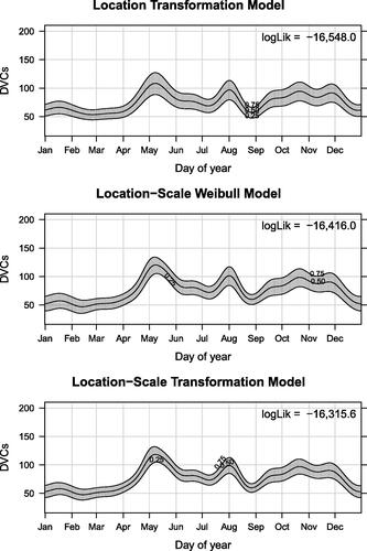
Assessing the temporal changes in DVC risk across a year, all three models are displayed on the quantile scale in Figure 4 for a hypothetical Monday in 2002. The curves reveal well-known seasonal patterns of increased DVC risk in April, July, and August due to increased animal activity. The plots further indicate that for the location transformation model large median values are associated with larger dispersion. This is not the case for the other two models, indicating a certain degree of underdispersion. The median annual risk pattern is very similar in all three models, however, the distribution-free location-scale transformation model reveals smaller variance compared to the other two models.

Fig. 4 Partial proportional hazards. Three annual quantile functions (0.25, 0.50, and 0.75th quantile) for DVCs (for a hypothetical Monday in 2002) estimated by three transformation models of increasing complexity. The in-sample log-likelihoods of the corresponding models are given in the panels.

The partial proportional hazards location-scale transformation model further allows investigation of the general trend of DVCs over a decade. From the log-hazard ratios ${\beta }_{\text{year}}$ we computed multiple comparisons of hazard ratios comparing subsequent years, with multiplicity control. Table 1 is in line with an increasing DVC risk from 2002 to 2004, followed by a plateau in 2005 and 2006, a further risk increase in 2007, and then plateauing in the remaining years.

Table 1 Partial proportional hazards.

Year	Hazard ratio	95% CI
2003–2002	0.66	0.53–0.81
2004–2003	0.74	0.60–0.91
2005–2004	0.92	0.75–1.13
2006–2005	1.12	0.91–1.38
2007–2006	0.58	0.47–0.72
2008–2007	0.88	0.72–1.09
2009–2008	0.99	0.80–1.21
2010–2009	0.99	0.80–1.21
2011–2010	1.08	0.88–1.32

NOTE: Estimates and corresponding simultaneous 95% confidence intervals (CI) of multiplicative changes in hazards by year. Hazard ratios smaller one indicate increasing DVCs when comparing two subsequent years.

3.2 Location-Scale Transformation Trees

Pollet and Nettle (2009) analyzed the self-reported orgasm frequency of 1533 Chinese women with current male partners. The ordinal outcome Y was reported in terms of ordered categories: never < rarely < sometimes < often < always. To assess the effect of explanatory variables on the distribution of reported orgasm frequencies, we reanalyze this data using a tree-structured location-scale transformation model. Explanatory variables included in the model are: partner income, partner height, duration of the relationship, respondents age (Rage), difference between education and wealth between both partners, the respondents education (Reducation: no school < primary school < lower-middle school < upper-middle school < junior college < university), health, happiness (Rhappy: very unhappy < not too unhappy < relatively happy < very happy) and place of living (Rregion).

We apply a modification of the transformation tree induction algorithm by Hothorn and Zeileis (2021) to estimate the location-scale transformation tree: (i) Fit an unconditional transformation model, (ii) assess the correlation of model scores and explanatory variables, (iii) find an appropriate binary split in the explanatory variable strongest correlated to the scores, (iv) proceed recursively. The novelty here is that location-scale trees pay attention to bivariate location-scale scores exclusively, instead of the P scores for the transformation parameters $\vartheta$ (as in Hothorn and Zeileis 2021). As in Section 3.1.2, the unconditional model $$\begin{array}{c}\mathbb{P}(Y\le y)=F\left(\sqrt{\hspace{0.17em}\exp \hspace{0.17em}(\gamma )}\mathit{a}{(y)}^{\top }\vartheta -\beta \right),\\ \mathrm{\hspace{1em}}\mathrm{\hspace{1em}}\text{subject to }\hspace{1em}\beta =\gamma =0\end{array}$$is fitted in each node of the tree by optimizing the likelihood $$\begin{array}{c}\widehat{\vartheta }=\text{arg} {\max }_{\vartheta }\sum _{i=1}^N{\mathcal{l}}_i(\vartheta ,0,1),\\ \mathrm{\hspace{1em}}\mathrm{\hspace{1em}}\text{subject to }{\vartheta }_p\le {\vartheta }_{p+1},p\in 1,\dots ,P-1.\end{array}$$

The bivariate score contributions are defined by $${\mathit{r}}_i={\frac{\partial {\mathcal{l}}_i\left(\vartheta ,\beta ,{\sqrt{\hspace{0.17em}\exp \hspace{0.17em}(\gamma )}}^{-1}\right)}{\partial (\beta ,\gamma )}|}_{\vartheta =\widehat{\vartheta },\beta =0,\gamma =0}\in {\mathbb{R}}^2.$$

Permutation tests are then applied to assess the association between the jth explanatory variable based on a quadratic form collapsing the linear test statistic ${\sum }_{i=1}^N{g}_j({\mathit{x}}_i){\mathit{r}}_i^{\top }\in {\mathbb{R}}^{Q(j)\times 2}$, where $g_j({\mathit{x}}_i)$ is a Q(j)-dimensional vector representing the jth explanatory variable of the ith subject. The bivariate score allows the tree to detect location and scale effects, for the model in Figure 5 on the logit scale. A p-value is computed for all $j=1,\dots ,J$ explanatory variables and the variable with minimum p-value is selected for splitting.

Fig. 5 Location-scale transformation tree. Female orgasm frequency in heterosexual relationships as a function of questionnaire variables reported by the female respondent.

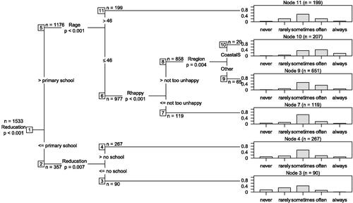
The location-scale transformation tree (Figure 5) indicates that higher orgasm frequencies were in general reported from higher educated, happier, and younger females. In this subgroup, the coastal south region was associated with a tendency to higher reported orgasm frequencies compared to the rest of China.

3.3 Transformation Additive Models for Location and Scale

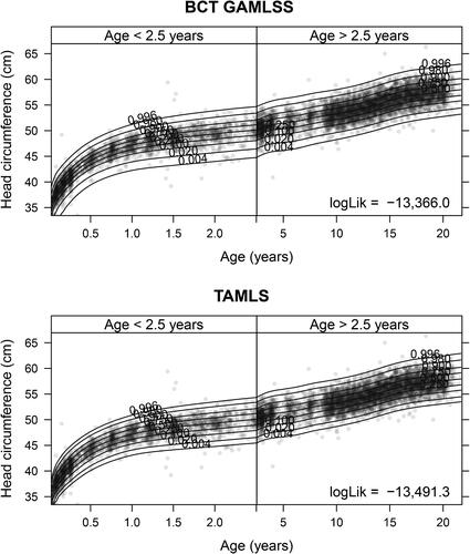
The head-circumference growth chart obtained from the Dutch growth study (Fredriks et al. 2000) is one of the standard examples in the GAMLSS literature. The top panel of Figure 6 shows the head-circumference quantiles for boys conditional on age obtained from fitting a GAMLSS with Box-Cox-t distribution, featuring four model terms $\mu (\text{age}),\sigma (\text{age}),\nu (\text{age})$, and $\tau (\text{age})$ (reproducing Figure 16 in Stasinopoulos and Rigby 2007). In our reanalysis, we replace the four parameter Box-Cox-t GAMLSS with a distribution-free transformation additive model for location and scale (TAMLS) featuring a conditional distribution function $$\mathbb{P}(Y\le y\mid \text{Age}=\text{age})=\Phi \left(\sigma {(\text{age})}^{-1}{\mathit{a}}_{\text{Bs},6}{(y)}^{\top }\vartheta -\mu (\text{age})\right)$$for head-circumference $Y\in {\mathbb{R}}^{+}$.

Fig. 6 Transformation additive models for location and scale (TAMLS). Conditional quantiles of head circumference along age estimated by the Box-Cox-t GAMLSS (BCT GAMLSS, top panel) and the TAMLS (bottom panel). The former model comprises four and the latter model two smooth terms.

In contrast to the GAMLSS, there is no need to assume a specific parametric distribution in the TAMLS and only two instead of four smooth terms have to be estimated. In this model, the transformation parameters $\vartheta$ can be understood as nuisance parameters. We employ the Rigby and Stasinopoulos (RS) algorithm (Rigby and Stasinopoulos 2005) developed for GAMLSS to estimate the two smooth terms $\mu (\text{age})$ and $\sigma (\text{age})$ in our TAMLS. For a given likelihood depending on a location and scale term, this algorithm allows estimation of these two terms in a structured additive way. We shield the more complex formulation of our model from the RS algorithm by setting-up a profile likelihood which, under the hood, estimates the nuisance parameters $\vartheta$ given μ and σ controlled by the RS algorithm. More specifically, for candidate functions μ and σ, the profile likelihood over $\vartheta$ is given by $$\begin{array}{c}\mathcal{l}(\mu (·),\sigma (·))=\text{arg} {\max }_{\vartheta }\sum _{i=1}^N{\mathcal{l}}_i(\vartheta ,\mu ({\mathit{x}}_i),\sigma ({\mathit{x}}_i))\\ \mathrm{\hspace{1em}}\mathrm{\hspace{1em}}\text{subject to }{\vartheta }_p\le {\vartheta }_{p+1},p\in 1,\dots ,P-1.\end{array}$$

We used log-likelihood contributions (3) in this specific application. Augmented Lagrangian Minimization (Madsen et al. 2004) was used to estimate $\vartheta$ given $\mu (·)$ and $\sigma (·)$. The penalized profile likelihood was optimized with respect to the two functions $\mu (·)$ and $\sigma (·)$ in Step 2a(i) of the RS algorithm (Appendix B, Rigby and Stasinopoulos 2005). The in-sample log-likelihood of the four term Box-Cox-t GAMLSS is slightly larger than the one of the distribution-free TAMLS, but the conditional quantile sheets obtained from the two models are very close and hardly distinguishable for boys older than 2.5 years (Figure 6).

Models assuming additivity of multiple smooth terms for the location effect $\mu (\mathit{x})={\sum }_{j=1}^J{m}_j(\mathit{x})$ and the scale effect $-2\hspace{0.17em}\log \hspace{0.17em}(\sigma (\mathit{x}))={\sum }_{l=1}^L{s}_l(\mathit{x})$ can be fitted by maximizing the same profile likelihood using the RS algorithm or L₂ boosting (for GAMLSS, Mayr et al. 2012). In this sense, transformation models introduce a novel distribution-free member to the otherwise strictly parametric GAMLSS family.

3.4 Model Selection

In the following we aim to assess the effect of explanatory variables on the medical demand by the elderly, that is, number of physician visits $Y=0,1,2,\dots$ for patients aged 66 or older, using a sample from the United States National Medical Expenditure Survey conducted in 1987 and 1988 (Deb and Trivedi 1997).

For such applications, location-scale transformation models (2) are especially attractive for parameter interpretation when linear location and scale terms are considered, and variables of special interest are present in the location term only (Section 2.1). If continuous explanatory variables $\mathit{x}$ are present in the model, a parameter identification issue arises which has previously been discussed in the GAMLSS context (Rigby et al. 2019,p. 60). In a location-scale model, $$\mathbb{P}(Y\le y\mid \mathit{X}=\mathit{x})=F\left(\sqrt{\hspace{0.17em}\exp \hspace{0.17em}({\mathit{x}}^{\top }\mathit{\gamma })}h(y\mid \vartheta )-{\mathit{x}}^{\top }\mathit{\beta }\right)$$the intercept, which is implicit in the transformation function $h(y\mid \vartheta )=\overline{h}(y\mid \overline{\vartheta })-{\beta }_0$, must not be multiplied with the scale term and an explicit intercept must be added to the location term, changing the model to (5) $$\mathbb{P}(Y\le y\mid \mathit{X}=\mathit{x})=F\left(\sqrt{\hspace{0.17em}\exp \hspace{0.17em}({\mathit{x}}^{\top }\mathit{\gamma })}\overline{h}(y\mid \overline{\vartheta })-{\beta }_0-{\mathit{x}}^{\top }\mathit{\beta }\right).$$(5)

The two models are not equivalent, but adding ${\beta }_0$ to h leads to an unidentified parameter when $\mathit{\gamma }$ is close to zero and omitting ${\beta }_0$ leads to different model fits when a constant is added to a continuous explanatory variable (e.g., when defining a suitable baseline distribution). For discrete parameterizations the expression for $\overline{h}$ simplifies to $\overline{h}(y\mid \vartheta )=\mathit{a}{(y)}^{\top }\vartheta$ with ${\vartheta }_1\equiv 0$. For polynomials in Bernstein form we have the following expression for $h(y\mid \vartheta )$: $$\begin{array}{c}{\mathit{a}}_{\text{Bs},P-1}{(y)}^{\top }\vartheta =\sum _{p=1}^P{a}_p(y){\vartheta }_p\\ =\sum _{p=1}^{P-1}(a_p(y)-a_P(y)){\overline{\vartheta }}_p+P^{-1}\sum _{p=1}^P{\vartheta }_p\\ =\overline{h}(y\mid \overline{\vartheta })-{\beta }_0\end{array}$$and ${\int }_{\mathbb{R}}\overline{h}(y\mid \overline{\vartheta }) dy=0$ because $a_p(·)$ are densities. The model parameters $\overline{\vartheta }$, $\mathit{\gamma }$, and $\mathit{\beta }$ can be estimated by maximizing the likelihood (after suitable adjustment to the constraints). However, for the sake of interpretability we aim to drop variables from the scale term whenever possible and therefore apply the L₀ penalty (detailed in Section 2.4, implemented in package tramvs (Kook 2023)) on $\mathit{\gamma }$ to the likelihood of model (5).

Applying the two estimation procedures, maximum likelihood and best subset selection, to a location-scale transformation model (with $F={\text{cloglog}}^{-1}$) estimating the effect of self-perceived health status (Health), sex (Sex), insurance coverage (Insurance), and the number of chronic conditions (Chronic) and years of education of patients (School) on the frequency of physician visits, allows for a head-to-head comparison of the parameter estimates (Table 2). In the best subset location-scale transformation model the variables Health, Sex, and School are dropped from the scale term allowing to interpret their effects in terms of (log-)hazard ratios. For the variable Sex, for example, the corresponding $\hspace{0.17em}\exp \hspace{0.17em}(-\widehat{\beta })=1.1333$ can be interpreted as hazard ratio comparing the hazards of male patients to the hazards of female patients, all other variables being equal.

Table 2 Model selection.

		ML		BSS
Variable	Level	$\widehat{\beta }$	$\widehat{\gamma }$	$\widehat{\beta }$	$\widehat{\gamma }$
Health	poor	0.3315	$-0.0912$	0.3997	—
	excellent	$-0.3722$	0.0417	$-0.2214$	—
Sex	male	$-0.1585$	$-0.2669$	$-0.1251$	—
Insurance	yes	0.2675	0.2541	0.2800	0.2272
Chronic		0.2542	0.1799	0.2729	0.2260
School		0.0234	$-0.0175$	0.0233	—

NOTE: Location and scale parameter estimates, $\widehat{\beta }$ and $\widehat{\gamma }$, from applying the two estimation procedures, maximum likelihood (ML) or best subset selection (BSS), to a location-scale transformation model including the following explanatory variables: Health (poor < average (baseline) < excellent), Sex (female (baseline), male), Insurance (no (baseline), yes), Chronic (number of chronic conditions) and School (number of years of education). Variables which were dropped when applying best subset selection are indicated by—.

4 Discussion

Tosteson and Begg (1988) introduced the notion of distribution-free location-scale regression in the context of ROC analysis. While they were able to estimate a corresponding model for ordinal responses, they contemplated that for models (2), “there is, as yet, no software for accommodating continuous test results, which are common outcomes for laboratory tests” (Tosteson and Begg 1988). With the introduction of a smooth transformation function and corresponding software implementation in the tram add-on package (Hothorn et al. 2023), we address this long-standing issue. We derive likelihood and score contributions for all response types and discuss suitable inference procedures for various functional forms.

In a broader context, we contribute a new distribution-free member to the rich family of location-scale models. The model is unique in the sense that data analysts do not have to commit themselves to a parametric family of distributions before fitting the model. The flexibility of our approach comes from the pair of location and scale terms allowing interpretability of conditional distributions on various scales, including proportional odds or hazards. Despite the distribution-free nature, we parameterize the model such that simple maximum-likelihood estimation for all types of responses becomes feasible. Therefore, our implementation handles arbitrary responses, including bounded, mixed discrete-continuous, and randomly censored outcomes, in a native way. Among other diverse applications, our flexible approach can help to generalize Weibull location-scale models previously studied as a model for crossing hazards using GAMLSS, allows for over- or underdispersion to be explained by covariates in complex count regression models, adds a notion of dispersion to regression trees for complex responses, provides means to reduce the complexity of growth-curve models, and has important applications in ROC analysis (Sewak and Hothorn 2023).

Special care with respect to parameter interpretability is needed when formulating the model. Parameters in linear location terms are interpretable as log-odds or log-hazard ratios as long as there is no corresponding scale parameter. Thus, model selection becomes vitally important should the data analyst be interested in direct parameter interpretation. A novel approach to best subset selection was presented and empirically evaluated. Model interpretation is possible on other scales (e.g., probabilistic indices or conditional quantiles), yet constitutes probably the biggest challenge of location-scale transformation models.

All models discussed here are “distributional” in the sense that they formulate a proper distribution function. Via appropriate constraints, our software implementation ensures that fitted models also directly correspond to conditional distribution functions. This feature allows straightforward parametric bootstrap implementations. Alternative suggestions for location-scale ordinal regression do not necessarily lead to estimates which can be interpreted on the probability scale (Cox 1995; Tutz and Berger 2017, 2020).

Algorithmically, we stand on the shoulders of giants, because only minor modifications to well-established algorithms were necessary for enabling parameter estimation. We didn’t fully explore all possibilities here, and for example location-scale transformation forests building on Hothorn and Zeileis (2021) or functional gradient boosting for this class (Hothorn 2020) are interesting algorithms for smooth interaction modeling in potentially high-dimensional covariate spaces.

Supplementary Materials

The supplementary material for this article includes the following: (A) computational details, (B) a re-analysis of the example from Tosteson & Begg (1988), (C) details on the best subset selection algorithm, and (D) simulation experiments.

Author’s contributions

SS and TH developed the model and its parameterization. SS wrote the manuscript, analyzed all applications, and performed the simulation study. LK implemented best subset regression for linear location-scale transformation models. TH implemented the likelihood and score function in package mlt. All authors revised and approved the final version of the manuscript.

Acknowledgments

The authors would like to thank Christoph Blapp and Klaus Steigmiller for embedding location-scale transformation models into the literature and for a proof-of-concept implementation.

Disclosure Statement

The authors report there are no competing interests to declare.

Additional information

Funding

SS and TH acknowledge financial support by the Swiss National Science Foundation, Grant No. 200021_184603.

References

- Burke, K., and MacKenzie, G. (2017), “Multi-Parameter Regression Survival Modeling: An Alternative to Proportional Hazards,” Biometrics, 73, 678–686. DOI: 10.1111/biom.12625.
- Burke, K., Eriksson, F., and Pipper, C. B. (2020), “Semiparametric Multiparameter Regression Survival Modeling,” Scandinavian Journal of Statistics, 47, 555–571. DOI: 10.1111/sjos.12416.
- Burke, K., Jones, M. C., and Noufaily, A. (2020), “A Flexible Parametric Modelling Framework for Survival Analysis,” Journal of the Royal Statistical Society, Series C, 69, 429–457. DOI: 10.1111/rssc.12398.
- Cox, C. (1995), “Location-Scale Cumulative Odds Models for Ordinal Data: A General Non-linear Model Approach,” Statistics in Medicine, 14, 1191–1203. DOI: 10.1002/sim.4780141105.
- Deb, P., and Trivedi, P. K. (1997), “Demand for Medical Care by the Elderly: A Finite Mixture Approach,” Journal of Applied Econometrics, 12, 313–336. DOI: 10.1002/(sici)1099-1255(199705)12:3¡313::aid-jae440¿3.0.co;2-g.
- Farouki, R. T. (2012), “The Bernstein Polynomial Basis: A Centennial Retrospective,” Computer Aided Geometric Design, 29, 379–419. DOI: 10.1016/j.cagd.2012.03.001.
- Fredriks, A. M., van Buuren, S., Burgmeijer, R. J. F., Meulmeester, J. F., Beuker, R. J., Brugman, E., Roede, M. J., Verloove-Vanhorick, S. P., and Wit, J. (2000), “Continuing Positive Secular Growth Change in The Netherlands 1955–1997,” Pediatric Research, 47, 316–323. DOI: 10.1203/00006450-200003000-00006.
- Haslinger, C., Korte, W., Hothorn, T., Brun, R., Greenberg, C., and Zimmermann, R. (2020), “The Impact of Prepartum Factor XIII Activity on Postpartum Blood Loss,” Journal of Thrombosis and Haemostasis, 18, 1310–1319. DOI: 10.1111/jth.14795.
- Hothorn, T. (2020), “Transformation Boosting Machines,” Statistics and Computing, 30, 141–152. DOI: 10.1007/s11222-019-09870-4.
- Hothorn, T., and Zeileis, A. (2021), “Predictive Distribution Modelling Using Transformation Forests,” Journal of Computational and Graphical Statistics, 30, 144–148. DOI: 10.1080/10618600.2021.1872581.
- Hothorn, T., Hornik, K., van de Wiel, M. A., and Zeileis, A. (2006), “A Lego System for Conditional Inference,” The American Statistician, 60, 257–263. DOI: 10.1198/000313006X118430.
- Hothorn, T., Müller, J., Held, L., Möst, L., and Mysterud, A. (2015), “Temporal Patterns of Deer-Vehicle Collisions Consistent with Deer Activity Pattern and Density Increase but not General Accident Risk,” Accident Analysis & Prevention, 81, 143–152. DOI: 10.1016/j.aap.2015.04.037.
- Hothorn, T., Möst, L., and Bühlmann, P. (2018), “Most Likely Transformations,” Scandinavian Journal of Statistics, 45, 110–134. DOI: 10.1111/sjos.12291.
- Hothorn, T., Barbanti, L., and Siegfried, S. (2023), tram: Transformation Models. R package version 0.8-3, https://CRAN.R-project.org/package=tram.
- Kneib, T., Silbersdorff, A., and Säfken, B. (2023), “Rage against the Mean – A Review of Distributional Regression Approaches,” Econometrics and Statistics, 26, 99–123. DOI: 10.1016/j.ecosta.2021.07.006.
- Kook, L. (2023), tramvs: Optimal Subset Selection for Transformation Models. R package version 0.0-4, available at https://CRAN.R-project.org/package=tramvs.
- Lepage, Y. (1971), “A Combination of Wilcoxon’s and Ansari-Bradley’s Statistics,” Biometrika, 58, 213–217. DOI: 10.2307/2334333.
- Madsen, K., Nielsen, H. B., and Tingleff, O. (2004), Optimization with Constraints (2nd ed.), Technical University of Denmark. Available at http://www2.imm.dtu.dk/pubdb/p.php?4213.
- Mayr, A., Fenske, N., Hofner, B., Kneib, T., and Schmid, M. (2012), “Generalized Additive Models for Location, Scale and Shape for High Dimensional Data – A Flexible Approach based on Boosting,” Journal of the Royal Statistical Society, Series C, 61, 403–427. DOI: 10.1111/j.1467-9876.2011.01033.x.
- McCullagh, P. (1980), “Regression Models for Ordinal Data,” Journal of the Royal Statistical Society, Series B, 42, 109–127. DOI: 10.1111/j.2517-6161.1980.tb01109.x.
- McLain, A. C., and Ghosh, S. K. (2013), “Efficient Sieve Maximum Likelihood Estimation of Time-Transformation Models,” Journal of Statistical Theory and Practice, 7, 285–303. DOI: 10.1080/15598608.2013.772835.
- Peng, D., MacKenzie, G., and Burke, K. (2020), “A Multiparameter Regression Model for Interval-Censored Survival Data” Statistics in Medicine, 39, 1903–1918. DOI: 10.1002/sim.8508.
- Peterson, B., and Harrell, F. E. (1990), “Partial Proportional Odds Models for Ordinal Response Variables,” Journal of the Royal Statistical Society, Series C, 39, 205–217. DOI: 10.2307/2347760.
- Pollet, T. V., and Nettle, D. (2009), “Partner Wealth Predicts Self-Reported Orgasm Frequency in a Sample of Chinese Women,” Evolution and Human Behavior, 30, 146–151. DOI: 10.1016/j.evolhumbehav.2008.11.002.
- Rigby, R., Stasinopoulos, D. M., Heller, G., and De Bastiani, F. (2019), Distributions for Modeling Location, Scale, and Shape: Using GAMLSS in R, Boca Raton, FL: Chapman & Hall/CRC Press. DOI: 10.1201/9780429298547.
- Rigby, R. A., and Stasinopoulos, D. M. (2005), “Generalized Additive Models for Location, Scale and Shape,” Journal of the Royal Statistical Society, Series C, 54, 507–554. DOI: 10.1111/j.1467-9876.2005.00510.x.
- Schein, P. S., and Gastrointestinal Tumor Study Group. (1982), “A Comparison of Combination Chemotherapy and Combined Modality Therapy for Locally Advanced Gastric Carcinoma,” Cancer, 49, 1771–1777. DOI: 10.1002/1097-0142(19820501)49:9¡1771::aid-cncr2820490907¿3.0.co;2-m.
- Sewak, A., and Hothorn, T. (2023), “Estimating Transformations for Evaluating Diagnostic Tests with Covariate Adjustment,” Statistical Methods in Medical Research. Accepted for publication. DOI: 10.1177/09622802231176030.
- Siegfried, S., and Hothorn, T. (2020), “Count Transformation Models,” Methods in Ecology and Evolution, 11, 818–827. DOI: 10.1111/2041-210X.13383.
- Stasinopoulos, D. M., and Rigby, R. A. (2007), “Generalized Additive Models for Location Scale and Shape (GAMLSS) in R,” Journal of Statistical Software, 23, 1–46. DOI: 10.18637/jss.v023.i07.
- Thas, O., De Neve, J., Clement, L., and Ottoy, J.-P. (2012), “Probabilistic Index Models,” Journal of the Royal Statistical Society, Series B, 74, 623–671. DOI: 10.1111/j.1467-9868.2011.01020.x.
- Tosteson, A. N. A., and Begg, C. B. (1988), “A General Regression Methodology for ROC Curve Estimation,” Medical Decision Making, 8, 204–215. DOI: 10.1177/0272989x8800800309.
- Tutz, G., and Berger, M. (2017), “Separating Location and Dispersion in Ordinal Regression Models,” Econometrics and Statistics, 2, 131–148. DOI: 10.1016/j.ecosta.2016.10.002.
- Tutz, G., and Berger, M. (2020), “Non Proportional Odds Models are Widely Dispensable – Sparser Modeling based on Parametric and Additive Location-Shift Approaches,” arXiv 2006.03914, arXiv.org E-Print Archive.
- Zeng, D., and Lin, D. Y. (2007), “Maximum Likelihood Estimation in Semiparametric Regression Models with Censored Data,” Journal of the Royal Statistical Society, Series B, 69, 507–564. DOI: 10.1111/j.1369-7412.2007.00606.x.
- Zhu, J., Wen, C., Zhu, J., Zhang, H., and Wang, X. (2020), “A Polynomial Algorithm for Best-Subset Selection Problem,” Proceedings of the National Academy of Sciences, 117, 33117–33123. DOI: 10.1073/pnas.2014241117.