Convergence of adaptive FEM for some elliptic obstacle problem

Abstract

In this work, we treat the convergence of adaptive lowest-order FEM for some elliptic obstacle problem with affine obstacle. For error estimation, we use a residual error estimator from [D. Braess, C. Carstensen, and R. Hoppe, Convergence analysis of a conforming adaptive finite element method for an obstacle problem, Numer. Math. 107 (2007), pp. 455–471]. We extend recent ideas from [J. Cascon, C. Kreuzer, R. Nochetto, and K. Siebert, Quasi-optimal convergence rate for an adaptive finite element method, SIAM J. Numer. Anal. 46 (2008), pp. 2524–2550] for the unrestricted variational problem to overcome the lack of Galerkin orthogonality. The main result states that an appropriately weighted sum of energy error, edge residuals and data oscillations satisfies a contraction property within each step of the adaptive feedback loop. This result is superior to a prior result from Braess et al. (2007) in two ways: first, it is unnecessary to control the decay of the data oscillations explicitly; second, our analysis avoids the use of some discrete local efficiency estimate so that the local mesh-refinement is fairly arbitrary.

Keywords:

• adaptive finite element methods
• elliptic obstacle problems
• convergence analysis

AMS Subject Classifications::

• 65N12
• 65N30
• 65N50
• 65K15

1. Introduction

1.1. Prior work on convergence of adaptive FEM

Adaptive finite element methods for partial differential equations based on various types of a posteriori error estimators have been intensively studied and are now a standard tool in science and engineering (see, e.g. the monographs 1,2 and the references therein). As far as a posteriori error analysis for elliptic obstacle problems is concerned, we refer to 3–11.

In the case of elliptic boundary value problems, convergence of adaptive mesh-refining algorithms has first been proven in 12, followed by 13. The latter works considered the residual error estimator for a P1-finite element discretization of the Poisson problem. In 13, the convergence analysis is based on reliability and the so-called discrete local efficiency of the residual error estimator, which relies on an interior node property for the local mesh-refinement. The main idea of the convergence proof then is to show that the error is contractive up to the data oscillations. This concept attracted quite some attention in the literature for various applications, e.g. the p-Laplacian 14, edge elements 15, mixed methods 16, nonconforming elements 17, and obstacle problems 18,19.

For the Poisson problem, optimality of the adaptive algorithm from 13 was first shown in 20. Recently, Cascon et al. 21 presented a new convergence proof under weaker conditions. They showed that a weighted sum of error and error estimator satisfies a contraction property without requiring (discrete local) efficiency of the estimator. In particular, their proof avoided the interior node property of the local mesh-refinement, and they even proved optimality.

1.2. Contributions of current work

We consider the framework in 18, i.e. adaptive P1-finite elements for some elliptic obstacle problem with affine obstacle. The obstacle problem is a classic introductory example to study variational inequalities which represent a whole class of problems that often arise in physical and economical context. One major application is the oscillation of a membrane that must stay above a certain obstacle. Other examples are filtration in porous media or the Stefan problem (i.e. melting solids) (see, e.g. 22 and the references therein).

In order to explain the differences to 18, we first recall their main result: Let ϵ_ℓ = 𝒥(U _ℓ) − 𝒥(u) ≥ 0 denote the energy error, where u is the exact solution of the obstacle problem and U _ℓ is the finite element approximation in the ℓ-th step of the adaptive algorithm. Based on a residual error estimator ϱ_ℓ consisting only of edge jumps and inspired by Morin et al. 13, Braess et al. 18, Theorem 3] states that the ϱ_ℓ-steered adaptive mesh-refinement leads to

with osc_ℓ being the data oscillations (essentially across edges, cf (13)–(14) below) and with 0 < κ < 1 and C > 0 being ℓ-independent constants. It is thus a consequence of elementary calculus that osc_ℓ → 0 implies convergence ϵ_ℓ → 0 as ℓ → ∞. In 13,18, however, the convergence osc_ℓ → 0 of the data oscillations has to be guaranteed by the implementation. This is usually done by performing additional local refinements until for some fixed constant 0 < ϑ < 1. We stress, however, that 18 provides no mathematical foundation on this step since the edge oscillations osc_ℓ are non-local. It is a technical byproduct of this work that edge oscillations satisfy a contraction property (Lemma 3.3), and thus the aforementioned algorithm from 18 is well-defined (cf Section 3.3).

Moreover, the main ingredients of the proof of (1) in 18 are the reliability of the error estimator, its discrete local efficiency and the marking strategy introduced by Dörfler 12 ensuring an appropriate selection of edges and elements for refinement. The discrete local efficiency, however, strongly relies on the interior node property of the local mesh-refinement, and thus the validity of the convergence analysis is constrained by the refinement strategy.

We follow a different convergence approach, inspired by 21: our main result (Theorem 3.4, Corollary 3.5) states that the adaptive algorithm steered by , i.e. steered by edge jumps plus data oscillations, leads to

with a weighted sum and with 0 < γ, κ < 1 being ℓ-independent constants. Note that the choice of our combined estimator has another advantage compared to 18: from the linear case (cf [21, Section 6.2]), one knows that separate marking and refinement might lead to suboptimal convergence rates, whereas the combined marking strategy does not. Moreover, our result is fairly independent of the chosen mesh-refinement and does not need the interior node property as does the analysis in 18.

The first step for our proof of (2) is to show that the sequence of the estimators η_ℓ is contractive in the sense that

where C > 0 and q ∈ (0, 1) are certain ℓ-independent constants and |||·||| denotes the energy norm (Proposition 3.1). To show this, we exploit the definition of the error estimator η_ℓ, the marking strategy used, and basic properties of the local mesh-refinement. In addition and contrary to 21, our elementary analysis avoids to dominate the data oscillations osc_ℓ by the element residuals and is thus much more accurate if f is smooth but quantitatively large.

1.3. Outline of current work

In Section 2, we formulate the continuous and discrete obstacle problem, stated as energy minimization problems. Moreover, we recall the error estimator η_ℓ from 18 which is later on used to steer our adaptive algorithm, and state its reliability (Proposition 2.2). In Section 3.1, we recall the marking strategy and the local mesh-refinement used. As a consequence, we prove that the estimator η_ℓ satisfies an estimator reduction property (Proposition 3.1) (cf (3)). One major part of our proof is to show that the edge data oscillations are, in fact, contractive (Lemma 3.3). Finally, Section 3.2 states our version of the η_ℓ-steered adaptive mesh-refining algorithm (Algorithm 1) and proves the contraction result (2). In particular, the generated sequence of discrete solutions U _ℓ converges, in fact, to the continuous solution u (Theorem 3.4). A short Section 3.3 considers the algorithm of 18 and comments on improvements which are byproducts of our analysis (Theorem 3.8). A numerical experiment in Section 4 concludes this work.

2. Model problem

2.1. Continuous formulation of model problem

Let Ω be a bounded domain in ℝ² with polygonal boundary Γ ≔ ∂Ω. We define an obstacle on by the affine function χ with χ ≤ 0 on ∂Ω. By , we denote the set of admissible functions

which is convex, closed and non-empty. For given f ∈ L ²(Ω), we consider the energy functional

where the energy scalar product reads

and where

denotes the L ²-scalar product. By |||·|||, we denote the energy norm on induced by ⟨⟨·, ·⟩⟩. The minimization problem then reads as follows: find u ∈ 𝒜 such that

The following well-known abstract lemma, found e.g. in 23, Theorem II.2.1], states unique solvability of this problem and equivalence to some variational inequality.

Lemma 2.1

Let ℋ be a Hilbert space over ℝ with scalar product ⟨⟨·, ·⟩⟩ and induced norm |||·|||. For any closed, convex and non-empty subset 𝒜 of ℋ and any linear functional f ∈ ℋ*, there is a unique minimizer u ∈ 𝒜 of (8). This minimizer is equivalently characterized in terms of the following variational inequality: find u ∈ 𝒜 such that

for all v ∈ 𝒜.

2.2. Conforming discretization

For the numerical solution of (8), we consider conforming and shape regular triangulations 𝒯_ℓ of Ω and denote the standard P1-finite element space of globally continuous and piecewise affine functions by 𝒮¹(𝒯_ℓ). The finite-dimensional minimization problem then reads as follows: find U _ℓ ∈ 𝒜_ℓ ≔ 𝒜 ∩ 𝒮¹(𝒯_ℓ) such that

Note that 𝒜_ℓ is a non-empty, convex and closed subset of 𝒮¹(𝒯_ℓ). With the same arguments as for the continuous problem, (10) admits a unique solution U _ℓ ∈ 𝒜_ℓ.

Throughout all sections, the set of all interior edges E = T ⁺ ∩ T ⁻ for certain elements T ⁺, T ⁻ ∈ 𝒯_ℓ is denoted by ℰ_ℓ. The set of all edges of 𝒯_ℓ is denoted by . In particular, contains all boundary edges and provides some partition of Γ.

2.3. Reliable error estimator

Now, let u ∈ 𝒜 denote the continuous solution of (8) and U _ℓ ∈ 𝒜_ℓ be the discrete solution of (10) for some fixed triangulation 𝒯_ℓ. To steer the adaptive mesh-refinement, we use some residual-based error estimator

from 18: first, ϱ_ℓ(E)² denotes the weighted L ²-norms of the normal jump

with h _E  = diam(E) the length of E and [·] the jump over an interior edge E = T ⁺ ∩ T ⁻ ∈ ℰ_ℓ. Second, osc_ℓ(E)² denotes the data oscillations of f over E

with Ω_ℓ,E  = T ⁺ ∪ T ⁻ the patch associated with E and the corresponding integral mean of f. Finally, for edges E on the boundary, η_ℓ involves the weighted element residuals

where T ∈ 𝒯_ℓ is the unique element with E = ∂T ∩ Γ. The following proposition has essentially been shown in 18, where osc_ℓ(E) for boundary edges E ∈ ℰ_ℓ,Γ is, however, weighted by diam(T)² ∼ |T|. We will discuss this, up to shape regularity, equivalent definition later on (cf Corollary 3.5 in Section 3.2).

Proposition 2.2

The estimator η_ℓ from (11) is reliable in the sense that there holds

The constant C ₁ > 0 depends only on Ω and the shape of the elements in 𝒯_ℓ.

Proof

The upper bound is stated in 18, Theorem 1] and hinges on the fact that the obstacle is affine. To see the lower bound, we use the variational inequality (9). For v = U _ℓ, this gives

and concludes the proof.▪

Remark 1

Before proceeding we want to comment quickly on other error estimators for obstacle problems in the literature. In some works (see, e.g. 7,10, estimators that only contribute within the non-contact set are used. This has some advantages since, for example, obstacles with kinks can be treated. The analysis in this case, however, becomes much more involved. In particular, it is unclear how to show an estimator reduction, or a contraction property in the sense of Proposition 3.1 or Theorem 3.4, respectively. As a consequence, for those kinds of estimators, only a weaker convergence result 10 can be shown, but not a contraction which is a crucial ingredient for a possible optimality analysis.

3. A convergent adaptive algorithm

3.1. Estimator reduction

As usual, we employ the local contributions of η_ℓ from (12)–(14) to steer the adaptive algorithm. For marking, we use the marking strategy introduced by Dörfler 12. Contrary to 12,13,18, we mark simultaneously for ϱ_ℓ(E) and data oscillations osc_ℓ(E): given some parameter θ ∈ (0, 1), we seek a set of usually minimal cardinality such that

For the mesh-refinement, we use newest-vertex bisection, where we mark all edges E ∈ ℳ_ℓ for refinement. The refinement rules are shown in Figure 1, and the reader is also referred to 1, Chapter 4]. Besides uniform shape regularity of 𝒯_ℓ+1, there is a certain decay of the mesh-widths:

•	Marked edges E ∈ ℳℓ are split into two edges of half length.
•	If at least one edge E of an element T ∈ 𝒯ℓ is marked, T is refined into up to four son elements T′ ∈ 𝒯ℓ+1 with |T|/4 ≤ |T′| ≤ |T|/2 (cf Figure 1).

Figure 1. For each triangle T ∈ 𝒯, there is one fixed reference edge, indicated by the double line (left, top). Refinement of T is done by bisecting the reference edge, where its midpoint becomes a new node. The reference edges of the son triangles are opposite to this newest vertex (left, bottom). To avoid hanging nodes, one proceeds as follows: we assume that certain edges of T, but at least the reference edge, are marked for refinement (top). Using iterated newest vertex bisection, the element is then split into 2, 3 or 4 son triangles (bottom).

These observations are essential to prove the following result.

Proposition 3.1

Suppose that the set satisfies (16) and marked edges are refined as stated before. Then, there holds

with some contraction constant q ∈ (0, 1) which depends only on θ ∈ (0, 1). The constant C ₂ > 0 additionally depends on the shape of the elements in 𝒯₀.

For the convenience of the reader, the proof of Proposition 3.1 is split into two lemmas which estimate the decay of the different contributions of η_ℓ if the mesh 𝒯_ℓ is locally refined.

Lemma 3.2

According to the refinement of marked edges E ∈ ℰ_ℓ ∩ ℳ_ℓ, there holds

Proof

We define the set containing all edges obtained by refinement of marked edges. Then, one observes

where we have used that the jump [∂ _n U _ℓ] is zero on all edges E′ ∈ ℰ_ℓ+1 which lie inside an element T ∈ 𝒯_ℓ.▪

Lemma 3.3

Suppose that 𝒯_ℓ+1 is obtained by newest vertex bisection of 𝒯_ℓ. Then, independent of the set of marked edges, it holds that

Proof

The proof of (19) is considerably longer than for the prior contributions in (18). The reason is that local mesh-refinement leads to additional edges inside the refined elements T ∈ 𝒯_ℓ. This provides additional contributions to osc_ℓ+1, which have to be controlled. For each edge and each element T ∈ 𝒯_ℓ with |T ∩ Ω_ℓ+1,E | > 0, we define the quantity

For a boundary edge , this definition is understood with Ω_ℓ+1,E  ≔ T′ and , where T′ ∈ 𝒯_ℓ+1 is the unique element with E = ∂T′ ∩ Γ. Throughout the proof, f _ω = (1/|ω|) ∫_ω f dx denotes the integral mean of f over the measurable set ω. Note that the L ²-best approximation property of f _ω yields

whence

For each element A ∈ 𝒯_ℓ, only four cases occur: A is either not refined, i.e. A ∈ 𝒯_ℓ ∩ 𝒯_ℓ+1, or refined by either one, two or three bisections (cf Figure 2).

First, assume that an element A ∈ 𝒯_ℓ ∩ 𝒯_ℓ+1 is not refined. Let b, c, d ∈ ℰ_ℓ ∩ ℰ_ℓ+1 denote its three edges. We then define

By definition, we obtain

even with equality.

Second, assume that an element A ∈ 𝒯_ℓ with edges is refined by one bisection (cf Figure 2), where the edge c is split into and one additional edge is created. Moreover, A is split into elements A ₁, A ₂ ∈ 𝒯_ℓ+1 with area |A ₁| = |A ₂| = |A|/2. Let B, C, D ∈ 𝒯_ℓ be the neighbours of A along the edges , where for instance B = ∅ if is a boundary edge. Then,

The last term belongs to the new edge . We define

and observe that, by definition, (20) holds with equality.

Third, assume that an element A ∈ 𝒯_ℓ with edges is refined by two bisections (cf Figure 2), where the edges c, d are split into , respectively, and two new edges are created. Moreover, A is split into elements A ₁, A ₂, A ₃ ∈ 𝒯_ℓ+1 with area |A ₁| = |A|/2 and |A ₂| = |A ₃| = |A|/4. Let b, c, d and B, C, D be the same as in the previous case. Then,

The last two terms belong to the new edges and are roughly estimated by

We define

By definition, we again obtain (20).

Fourth, assume that an element A ∈ 𝒯_ℓ with edges is refined by three bisections (cf Figure 2), where the edges b, c, d are split into , respectively, and three new edges are created. Moreover, A is split into elements A ₁, A ₂, A ₃, A ₄ ∈ 𝒯_ℓ+1 with area |A _j | = |A|/4. For b, c, d and B, C, D, we use the notation from the previous cases. Then,

Defining

we again guarantee (20).

Now, it only remains to show that for non-refined edges holds

whereas for edges which are refined, there holds

Of course, there are quite some cases to be considered. Since all follow by direct calculation, we only consider some particular examples shown in Figure 3, while we refer to 24, Lemma 3.3.6] for the consideration of all possible cases.

We first consider b ≔ A ∩ B ∈ ℰ_ℓ. According to our definitions, there holds

This implies

Next, we consider d ≔ A ∩ D ∈ ℰ_ℓ. We have

This implies

Finally, we consider the boundary edge . In this case, there holds

and we also observe the contraction property.

Having obtained (21)–(22), we may proceed as follows: we note that (20) provides

Therefore, (21)–(22) show

and conclude the proof.▪

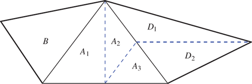
Figure 2. Refinement of an element A by one (a), two (b) or three (c) bisections and notation used in the proof of Lemma 3.3.

Figure 3. The element A ∈ 𝒯_ℓ is refined by two bisections. It has two neighbouring elements B, D ∈ 𝒯_ℓ, whereas the third edge is on the boundary.

Proof of Proposition 3.1

First, the triangle inequality in the sequence space ℓ₂ proves

In particular, the Young inequality yields for arbitrary δ > 0

Second, recall that . Using the estimates (18) and (19), we thus see

Third, the Dörfler marking (16) is used to obtain

Fourth, according to uniform shape regularity of the generated family (𝒯_ℓ)_ℓ∈ℕ, there holds

Plugging the last two estimates into (23), we prove (17), where we finally choose δ > 0 sufficiently small to guarantee q ≔ (1 + δ)(1 − θ/4) < 1.▪

Remark 1

Clearly, Lemma 3.2 also holds if certain elements T ∈ 𝒯_ℓ are refined by five bisections, as is done in 18, or by the so-called red-refinement. We refer to 1, Chap. 4] for details on different local mesh-refinements.

The same holds for Lemma 3.3 as well. In case of bisec₅-refinement this is easily seen as follows: we theoretically build an intermediate mesh 𝒯_ℓ+1/2, where elements marked for bisec₅ are only refined by three bisections. Then, Lemma 3.3 applies for the refinement from 𝒯_ℓ to 𝒯_ℓ+1/2. To finally obtain 𝒯_ℓ+1, certain elements T′ ∈ 𝒯_ℓ+1/2 have to be refined by one bisection. Note that this guarantees since only certain interior edges E′ ∈ ℰ_ℓ+1/2\ℰ_ℓ are effected. Since (19) states, in particular, monotone decay of the oscillations, we conclude

where osc_ℓ+1/2 denotes the oscillation term associated with the only theoretically constructed mesh 𝒯_ℓ+1/2.

Finally, if certain elements of 𝒯_ℓ are refined by red-refinement, the proof of (19) is obtained by similar calculations as in the proof of Lemma 3.3. We refer to 24 for details.

3.2. Convergent adaptive algorithm

In this section, we formally state our version of the adaptive algorithm and prove that it generates a sequence of discrete solutions U _ℓ which converge to the continuous minimizer u.

Algorithm 1

Fix 0 < θ < 1 and let 𝒯_ℓ with ℓ = 0 be the initial triangulation. For each ℓ = 0, 1, 2, … , do:

i.	Compute discrete solution U ℓ ∈ 𝒜ℓ ≔ 𝒜 ∩ 𝒮1(𝒯ℓ)
ii.	Compute indicators ηℓ(E) for all .
iii.	Determine set which satisfies (16).
iv.	Mark all edges E ∈ ℳℓ for refinement.
v.	Obtain new mesh 𝒯ℓ+1 by newest vertex bisection and increase counter ℓ ↦ ℓ + 1.

Theorem 3.4

Algorithm 1 guarantees that the combined error quantity

satisfies the contraction property

The constants 0 < γ, κ < 1 depend only on the parameter θ and the shape of the elements in 𝒯₀. In particular, there holds as well as .

Proof

According to Proposition 3.1, we have

with certain constants 0 < q < 1 and C ₂ > 0. Therefore,

Using the variational inequality (9) applied for U _ℓ+1, we proceed as in the proof of Proposition 2.2 to see

Choosing γ sufficiently small to guarantee γC ₂ − 1/2 ≤ 0, we then obtain

According to Proposition 2.2, there holds

For ϵ > 0, we thus observe

with . Since q < 1, we may choose ϵ > 0 sufficiently small to guarantee q + ϵ < 1. This choice leads to κ < 1, and we finally end up with (25). By induction, this implies

With reliability |||u − U _ℓ||| ≲ η_ℓ, we thus conclude the proof.▪

In 18, the weighting instead of |T| is used in the definition (14) of osc_ℓ(E), i.e.

where

and T ∈ 𝒯_ℓ is the unique element with E = ∂T ∩ Γ. Note that this definition does not necessarily yield a contraction h _T′ < h _T if an edge E ∈ ℰ_ℓ,Γ ∩ ℳ_ℓ is refined and T′ ∈ 𝒯_ℓ+1 is one of the resulting sons of T. Nevertheless, leads to a convergent adaptive FEM in the sense of Theorem 3.4.

Corollary 3.5

Suppose that instead of η_ℓ is used in Algorithm 1 for marking. Then, the modified algorithm still guarantees the contraction property (25). In particular, there holds as well as .

Proof

Note that there holds

with some constant C ₃ ≥ 1 which depends only on the shape regularity of the mesh 𝒯_ℓ. Since newest vertex bisection leads to uniformly shape regular meshes, C ₃ may be chosen independently of ℓ. The Dörfler marking (16) for thus implies

Put differently, the set ℳ_ℓ satisfies the Dörfler marking (16) for as well as the Dörfler marking (16) for , where . Therefore, Theorem 3.4 applies and (25) holds. In particular, and the equivalence (29) also concludes .▪

Remark 2

The estimator reduction (17) already implies convergence lim_ℓ η_ℓ = 0, whence lim_ℓ𝒥(U _ℓ) = 𝒥(u) as well as lim_ℓ|||u − U _ℓ||| = 0 according to Proposition 2.2. To see this, it remains to verify that the obstacle problem leads to a priori convergence lim_ℓ U _ℓ = u _∞ with a certain limit u _∞ ∈ ℋ. For linear problems, such a result is found in 25–27, and we refer to [24, Lemma 3.3.8] for the proof of the a priori convergence in our non-linear setting. Then, (17) takes the form

with the zero sequence α_ℓ = C ₂ |||U _ℓ+1 − U _ℓ|||² ≥ 0. Therefore, elementary calculus concludes lim_ℓη_ℓ = 0 (cf 25). We stress that, contrary to 27, the estimator reduction concept from 25 avoids any use of discrete efficiency. It is only based on the precise definition of the error estimator, a uniform decay of the mesh-width locally on marked elements, and the observation that any kind of mesh-refinement will lead to a convergent sequence of discrete solutions. We stress, however, that the convergence results in Theorem 3.4 and Corollary 3.5 are stronger since they include even a contraction of some error quantity Δ_ℓ ≥ ϵ_ℓ = 𝒥(U _ℓ) − 𝒥(u).

3.3. Convergence analysis for the adaptive algorithm from 18

In this section, we aim to comment briefly on the adaptive algorithm in 18 and improve their convergence result in several aspects.

Algorithm 2

Fix 0 < θ, ϑ < 1 and let 𝒯_ℓ with ℓ = 0 be the initial triangulation. For each ℓ = 0, 1, 2, … , do:

i.	Compute discrete solution U ℓ ∈ 𝒜ℓ ≔ 𝒜 ∩ 𝒮1(𝒯ℓ)
ii.	Compute indicators ϱℓ(E)2 as well as oscillation terms oscℓ(E) for all .
iii.	Determine set ℳℓ ⊆ ℰℓ which satisfies
iv.	Mark all edges E ∈ ℳℓ for refinement and obtain intermediate mesh 𝒯ℓ+1/2 by newest vertex bisection of 𝒯ℓ.
v.	Refine additional elements of 𝒯ℓ+1/2 and update 𝒯ℓ+1/2 until the corresponding oscillations satisfy oscℓ+1/2 ≤ ϑ oscℓ.
vi.	Finally, set 𝒯ℓ+1 ≔ 𝒯ℓ+1/2 and increase counter ℓ ↦ ℓ + 1.

In Braess et al. 18, the authors do not give further information on step (v) besides their choice θ = ϑ. In particular, it is not obvious how many levels of refinement have to be done until osc_ℓ+1 ≤ ϑ osc_ℓ is satisfied. In the following, we comment on a practical realization of (v) and derive a convergence result similar to Theorem 3.4. Our recommendation reads as follows:

	(v.a) If , define 𝒯ℓ+1 ≔ 𝒯ℓ+1/2
	(v.b) Otherwise determine such that
	(v.c) mark all edges E ∈ ℳℓ+1/2 for refinement,
	(v.d) and obtain new mesh 𝒯ℓ+1 by newest vertex bisection.

We first prove that this part guarantees contraction of the data oscillations.

Lemma 3.6

The proposed realization of step (v) in Algorithm 2 guarantees osc_ℓ+1 ≤ ϑ osc_ℓ with ϑ = (1 − θ/4)^1/2.

Proof

We may assume that since otherwise osc_ℓ+1/2 = osc_ℓ+1 by definition. Using Lemma 3.3 and arguing as in the proof of Proposition 3.1 (but only for the oscillation terms), we see that the marking criterion (31) guarantees . Since 𝒯_ℓ+1/2 is a refinement of 𝒯_ℓ, the monotonicity osc_ℓ+1/2 ≤ osc_ℓ of the edge oscillations concludes the proof.▪

Next, we prove an estimator reduction similar to Proposition 3.1.

Proposition 3.7

The extended Algorithm 2 from 18 guarantees

with constants q ∈ (0, 1) and C ₄ > 0 which depend only on θ ∈ (0, 1) and the shape of the elements in 𝒯₀.

Proof

Note that 𝒯_ℓ+1 is a refinement of 𝒯_ℓ+1/2, and 𝒯_ℓ+1/2 is a refinement of 𝒯_ℓ. Arguing as in the proof of Proposition 3.1 (but only for the edge jumps), we see that the modified marking criterion (30) yields

for all δ > 0. As above, the constant C > 0 stems from inverse-type estimates and depends only on the uniform shape regularity of the meshes involved. In view of the contraction from Lemma 3.6, we choose δ > 0 sufficiently small such that (1 + δ)²(1 − θ/2) ≤ (1 − θ/4). Adding the estimate of Lemma 3.6, we conclude the proof with q = (1 − θ/4).▪

Finally, we argue as in the proof of Theorem 3.4 to obtain the following convergence result whose proof is omitted for brevity. We stress that our result is superior to the convergence result from 18 for several reasons: First, we only need one bisection instead of five per refined element. Second, our recommendation of ϑ = (1 − θ/4)^1/2 satisfies ϑ ≥ θ for practical choices of θ, namely θ < 0.88. Third, our modification of their algorithm guarantees that at most one additional step of newest vertex bisection has to be performed to guarantee contraction of the oscillations.

Theorem 3.8

The extended Algorithm 2 from 18 guarantees

The constants 0 < γ, κ < 1 depend only on the parameter θ and the shape of the elements in 𝒯₀. In particular, there holds as well as .

4. Numerical experiment

In this section, we consider a numerical experiment from 18. The conforming and shape regular mesh is adaptively generated by Algorithm 1. For the solution of the discrete obstacle problem at each level, the primal-dual active set strategy from 28 has been used. For the initial mesh 𝒯₀, we choose for the primal dual pair as initial guesses for the iterative solver. For 𝒯_ℓ, we choose the prolongated discrete solutions associated with the previous mesh, i.e. as well as . We stop the iterative solver if the difference of two consecutive solutions satisfies

for some tolerance τ > 0, where N = #𝒯_ℓ denotes the number of elements. We then define our discrete solution at 𝒯_ℓ by and .

While the numerical results are quite similar to those in 18, we stress that our approach theoretically includes the data oscillations into the estimator η_ℓ.

We consider the obstacle problem with constant obstacle χ ≡ 0 on the L-shaped domain Ω ≔ (−2, 2)²∖ [0, 2) × (−2, 0]. The right-hand side is given in polar coordinates by

where (·)′ denotes the radial derivative d/dr. Moreover, and

Then, the exact solution reads in polar coordinates

and exhibits a corner singularity at the origin. We compare uniform and adaptive mesh-refinement, where we vary the adaptivity parameter θ ∈ {0.2, 0.4, 0.6, 0.8} in Algorithm 1. The quantities of interest are the energy error

as well as the error estimator η_ℓ from (11) which includes oscillations and edge jumps. Since the oscillations are, however, expected to be of higher order, the values of osc_ℓ are explicitly given.

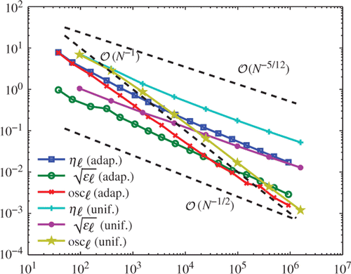
In Figure 4, we plot , η_ℓ and osc_ℓ over the number N = #𝒯_ℓ of elements for uniform and adaptive mesh-refinement with θ = 0.6. Uniform mesh-refinement leads to a suboptimal convergence behaviour with respect to the number N = #𝒯_ℓ of elements. Contrary, adaptive mesh-refinement regains the optimal order of convergence . We stress that the given data are smooth so that uniform as well as adaptive mesh-refinement leads to osc_ℓ = 𝒪(N ⁻¹), which corresponds to second-order convergence with respect to a uniform mesh-width. For both mesh-refinements, we see that the curves of η_ℓ and are parallel. This experimentally confirms the reliability of η_ℓ from Proposition 2.2 and indicates that η_ℓ is also efficient.

Figure 4. Numerical results for uniform and adaptive mesh-refinement with θ = 0.6, where ϵ_ℓ = 𝒥(U _ℓ) − 𝒥(u), η_ℓ and osc_ℓ are plotted over the number N = #𝒯_ℓ of elements.

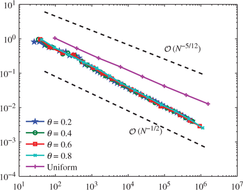
Figure 5 provides the experimental comparison for different values of θ ∈ {0.2, 0.4, 0.6, 0.8}. We see that each choice of θ leads to optimal order of convergence and that the corresponding curves essentially coincide. Since achievement of a prescribed precision takes much longer with uniform refinement, the benefits of adaptive refinement are clearly visible. Additionally, we stress that also the convergence rate itself is improved.

Figure 5. Numerical results for for uniform and adaptive mesh-refinement with θ ∈ {0.2, 0.4, 0.6, 0.8}, plotted over the number N = #𝒯_ℓ of elements.

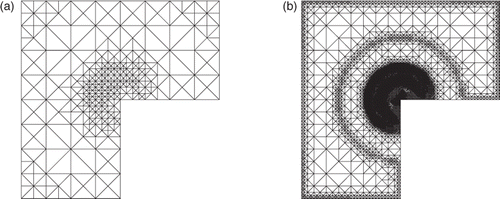
Figure 6 displays the adaptively generated meshes 𝒯₅ and 𝒯₁₁, respectively for θ = 0.6. As expected, refinement is basically restricted to the inactive zone. Due to the data oscillation terms in the estimator η_ℓ, we also observe certain refinement within the active zone. Note that the corresponding figures in 18 do not show any refinement inside the active zone. We stress, however, that those figures are somewhat misleading in the following sense: the right-hand side f is non-zero along the boundary in this example. Therefore, the contraction of the overall oscillations (as it is postulated by 18) can only be achieved if (sooner or later) refinements take place also within the active zone. The algorithm from 18 will thus eventually lead to the very same refinement along the boundary that we observe here.

Figure 6. Adaptively generated meshes 𝒯₅ (a) and 𝒯₁₁ (b) with N = 568 and N = 22140 elements, respectively, for θ = 0.6.

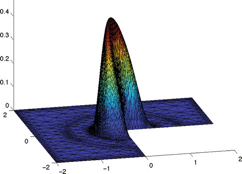
Finally, the numerical solutions after eight steps of refinement is shown in Figure 7.

Figure 7. Galerkin solution U ₈ on adaptively generated mesh 𝒯₈ with N = 3524 elements for θ = 0.6.

Acknowledgements

The authors acknowledge support of the Viennese Science and Technology Fund (WWTF) through the research project MA09–029 Micromagnetic Simulation and Computational Design of Future Devices. The second author (D.P.) acknowledges support of the Austrian Science Fund (FWF) through the project Adaptive Boundary Element Method under grant P21732.

References

- Verfürth , R . 1996 . A Review of a Posteriori Error Estimation and Adaptive Mesh-refinement Techniques , New York : Wiley-Teubner .
- Ainsworth , M and Oden , T . 2000 . A Posteriori Error Estimation in Finite Element Analysis , New-York : Wiley-Interscience .
- Ainsworth , M , Lee , C and Oden , T . 1993 . Local a posterori error estimators for variational inequalities . Numer. Meth. Part. D. E. , 9 : 23 – 33 .
- Braess , D . 2005 . A posteriori error estimators for obstacle problems – Another look . Numer. Math. , 101 : 415 – 421 .
- Bartels , S and Carstensen , C . 2004 . Averaging techniques yield reliable a posteriori finite element error control for obstacle problems . Numer. Math. , 99 : 225 – 249 .
- Chen , Z and Nochetto , R . 2000 . Residual type a posteriori error estimates for elliptic obstacle problems . Numer. Math. , 84 : 527 – 548 .
- Gräser , C , Kornhuber , R , Veeser , A and Zou , Q . 2011 . Hierarchical error estimates for the energy functional in obstacle problems . Numer. Math. , 117 : 653 – 677 .
- Liu , W and Yan , N . 2000 . A posteriori error estimates for a class of variational inequalities . J. Sci. Comput. , 15 : 361 – 393 .
- Nochetto , R , Siebert , K and Veeser , A . 2005 . Fully localized a posteriori error estimators and barrier sets for contact problems . SIAM J. Numer. Anal. , 42 : 2118 – 2135 .
- Siebert , K and Veeser , A . 2007 . A uniliterally constrained quadratic minimization with adaptive finite elements . SIAM. J. Optim. , 18 : 260 – 289 .
- Veeser , A . 2001 . Efficient and reliable a posteriori error estimators for elliptic obstacle problems . SIAM J. Numer. Anal. , 39 : 146 – 167 .
- Dörfler , W . 1996 . A convergent adaptive algorithm for Poisson's equation . SIAM J. Numer. Anal. , 33 : 1106 – 1124 .
- Morin , P , Nochetto , R and Siebert , K . 2000 . Data oscillation and convergence of adaptive FEM . SIAM. J. Numer. Anal. , 18 : 466 – 488 .
- Veeser , A . 2002 . Convergent adaptive finite elements for the nonlinear Laplacian . Numer. Math. , 92 : 743 – 770 .
- Carstensen , C and Hoppe , R . 2005 . Convergence analysis of an adaptive edge finite element method for the 2D eddy current equations . J. Numer. Math. , 13 : 19 – 32 .
- Carstensen , C and Hoppe , R . 2006 . Error reduction and convergence for an adaptive mixed finite element method . Math. Comp. , 75 : 1033 – 1042 .
- Carstensen , C and Hoppe , R . 2006 . Convergence analysis of an adaptive nonconforming finite element method . Numer. Math. , 103 : 251 – 266 .
- Braess , D , Carstensen , C and Hoppe , R . 2007 . Convergence analysis of a conforming adaptive finite element method for an obstacle problem . Numer. Math. , 107 : 455 – 471 .
- Braess , D , Carstensen , C and Hoppe , R . 2009 . Error reduction in adaptive finite element approximations of elliptic obstacle problems . J. Comput. Math. , 27 : 148 – 169 .
- Stevenson , R . 2007 . Optimality of standard adaptive finite element method . Found. Comput. Math. , 3 : 245 – 269 .
- Cascon , J , Kreuzer , C , Nochetto , R and Siebert , K . 2008 . Quasi-optimal convergence rate for an adaptive finite element method . SIAM J. Numer. Anal. , 46 : 2524 – 2550 .
- Friedman , A . 1982 . Variational Principles and Free-boundary Problems , New York : Wiley .
- Kinderlehrer , D and Stampacchia , G . 1980 . An Introduction to Variational Inequalities , New York : Academic Press .
- Page , M . 2010 . “ Schätzerreduktion und Konvergenz adaptiver FEM für Hindernisprobleme ” . In Master thesis (in German) , Wien : Institute for Analysis and Scientific Computing, Vienna University of Technology .
- Aurada , M , Ferraz-Leite , S and Praetorius , D . 2009 . Estimator reduction and convergence of adaptive FEM and BEM , Wien : ASC Report 27/2009, Institute for Analysis and Scientific Computing, Vienna University of Technology .
- Carstensen , C and Praetorius , D . 2009 . Convergence of adaptive boundary element methods, ASC Report 15/2009 , Wien : Institute for Analysis and Scientific Computing, Vienna University of Technology .
- Morin , P , Siebert , K and Veeser , A . 2008 . A basic convergence result for conforming adaptive finite elements . Math. Models Methods Appl. Sci. , 18 : 707 – 737 .
- Hintermüller , M , Ito , K and Kunisch , K . 2003 . The primal-dual active set strategy as a semismooth newton method . SIAM J. Optim. , 13 : 865 – 888 .