
 ?Mathematical formulae have been encoded as MathML and are displayed in this HTML version using MathJax in order to improve their display. Uncheck the box to turn MathJax off. This feature requires Javascript. Click on a formula to zoom.
ABSTRACT
We consider the nonsteady flow of a micropolar fluid in a thin (or long) curved pipe via rigorous asymptotic analysis. Germano's reference system is employed to describe the pipe's geometry. After writing the governing equations in curvilinear coordinates, we construct the asymptotic expansion up to a second order. Obtained in the explicit form, the asymptotic approximation clearly demonstrates the effects of pipe's distortion, micropolarity and the time derivative. A detailed study of the boundary layers in space is provided as well as the construction of the divergence correction. Finally, a rigorous justification of the proposed effective model is given by proving the error estimates.
COMMUNICATED BY:
1. Introduction
The model of micropolar fluids was first introduced in 1960s by Eringen in his well-known paper [Citation1], providing a generalization of the classical Navier–Stokes model. The main advantage of the micropolar fluid model is due to the fact that it takes into account the microstructure of the fluid particles and effects such as rotation and shrinking. Consequently, numerous non-Newtonian fluids such as liquid crystals, animal blood, muddy fluids and even water in small scales can be described in a more precise and realistic manner. In order to describe the rotation of the particles, a new vector field is introduced – the angular velocity field of rotation (microrotation), and accordingly a new equation coming from the conservation of the angular momentum. In this way, we obtain a coupled system of partial differential equations with four new viscosity coefficients. The model of micropolar fluids has been a subject of research in both the mathematical and engineering community: a comprehensive survey of the underlying mathematical theory can be found in the monograph by Lukaszezwicz [Citation2], whereas recent results concerning engineering applications in biomedicine and blood flow modelling can be found in [Citation3–8].
In last two decades, one can also find a number of papers providing a rigorous derivation of new asymptotic models for steady-state flows in thin domains. The model describing the flow of Newtonian fluid in a three-dimensional curved pipe has been formally derived and justified via error estimate by Marušić–Paloka [Citation9]. The asymptotic behaviour of a steady flow in a system of thin pipes has been considered by the same author in [Citation10]. The steady flow of a micropolar fluid has been investigated by Dupuy, Panasenko and Stavre [Citation11,Citation12] in two-dimensional domains such as a periodically constricted tubes and curvilinear channels. A three-dimensional setting including an undeformed pipe and a curved pipe has been addressed by Pažanin [Citation13,Citation14], while multiple pipe system has been treated by Beneš and Pažanin [Citation15].
Most recently, new asymptotic models for the nonsteady flows have been proposed and mathematically justified in case of classical, Newtonian fluid by Panasenko and Pileckas [Citation16–18] in an infinite cylinder and a system of thin pipes. The asymptotic behaviour of nonsteady Newtonian fluid flow in a curved three-dimensional thin pipe with moving walls has been considered by Castineira et al. [Citation19,Citation20]). A higher-order model describing the nonsteady flow of a micropolar fluid through a straight pipe has been rigorously derived in [Citation21,Citation22] by the authors of this paper. In view of that and inspired by the applications, our aim here is to investigate a nonsteady micropolar flow through a pipe with an arbitrary (generic) central curve.
The paper is organized as follows. In Section 2, we formally describe the geometry of the curved pipe using Germano's frame of reference (introduced in [Citation23,Citation24]) and consider the equations describing the nonsteady micropolar fluid flow. In Section 3, we introduce the curvilinear coordinates and rewrite the governing problem in an undeformed pipe. In Section 4, using two-scale expansion technique, we compute the asymptotic approximation up to a second-order in order to capture the effects of the pipe's geometry, micropolarity as well as the time derivative. It should be emphasized that the asymptotic solution is provided in the form of the explicit formulae, which is particularly important with regards to numerical simulations. We also conduct a detailed boundary layer analysis in the vicinity of pipe's ends and construct the divergence correction to improve the order of accuracy of our model. In Section 5, we prove the error estimates in suitable norms evaluating the difference between the exact solution of the problem (which cannot be found due to the complexity of the flow domain and the equations) and our second-order asymptotic approximation. By doing that, we justify the usage of the proposed effective model and that represents our main contribution. We strongly believe that the presented result can be useful in the practice, especially one related to blood flow modelling. Finally, in the appendix, we provide complete expressions computed for the higher-order regular part correctors as well as for the exponentially decreasing functions appearing in the boundary layers problems.
2. The setting of the problem
2.1. Description of the pipe's geometry
In the following, we define our thin (or long) curved pipe with a smooth central curve γ and a circular cross-section. We suppose that the curve γ is a generic curve in
parameterized by its arc length
. We denote by
its natural parametrization such that
, for every
. At each point,
of the curve γ we define its curvature (flexion) as
and introduce Frenet's basis by
where
is the tangent,
the normal and
the binormal. The torsion of γ is denoted by
. It is known that the Frenet's basis
satisfies the system
(1)
(1) Let
be a small parameter and
a unit circle. We define the undeformed thin pipe as
Next, we introduce the mapping
by
(2)
(2) where
(3)
(3) and
(4)
(4) with
and
being arbitrary constants. The local injectivity of
can be easily established assuming ε is sufficiently small (see [Citation14, Section 3.1] for details).
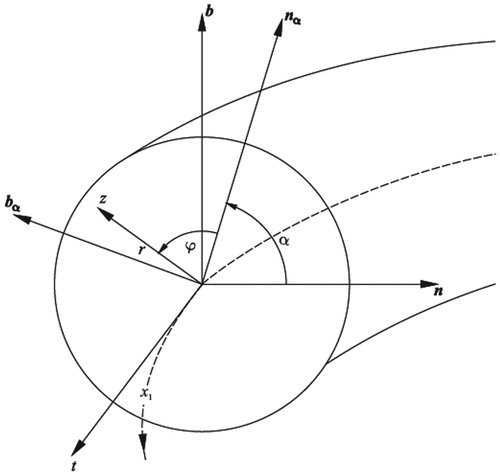
Figure 1. Germano's frame of reference.
We can now define the curved pipe with the central curve γ and circular cross-section by putting
We also denote by
the ends of the pipe and by
its lateral boundary.
2.2. The flow equations
The equations describing the nonsteady flow of a micropolar fluid in a thin curved pipe read:
(5)
(5)
Here
is the velocity field,
is the pressure and
is the microrotation field. The external sources of linear and angular momentum are given by the functions
and
, where
. We employ the notation
,
,
and
, where ν is the Newtonian viscosity,
is the microrotation viscosity, while
and
are the coefficients of angular viscosities.
We prescribe the following boundary and initial condition:
(6)
(6) where we suppose that the prescribed velocities
are given in the form
(7)
(7) where
, and
(8)
(8) where
. To assure the well-posedness of the governing problem, the following compatibility condition needs to be fulfilled:
(9)
(9) Since the initial velocity equals to zero, there also needs to hold
(10)
(10) In the following, we suppose that
and
vanish in the neighbourhood of t=0, i.e.
(11)
(11) Let
and
for j=0,1 and let
with
be the solution of the following problem (see Lemma 5.2):
A weak solution of our problem (Equation5
(5)
(5) )–(Equation11
(11)
(11) ) is a pair
such that
, and
satisfy the integral identities
(12)
(12) Let
,
. There then exists a unique weak solution
satisfying (12) for a.e.
. The proof follows the same arguments as the proof of Theorem 2.1.1 from [Citation2, Chapter III, Section 2] which can be straighforwardly adapted to our setting.
3. Rewriting the problem
In this section, we will provide the geometric tools necessary to write the problem (Equation5(5)
(5) )–(Equation11
(11)
(11) ) on the reference domain
, allowing us to perform the asymptotic analysis.
3.1. Covariant and contravariant basis
Let us consider the following mapping:
We introduce the covariant basis as the gradient of the mapping
consisting of vectors
Using (Equation2
(2)
(2) )–(Equation3
(3)
(3) ) and Frenet's relations (Equation1
(1)
(1) ), one can easily obtain
where
(13)
(13) From (Equation4
(4)
(4) ), it directly follows that
, so we have
The contravariant basis is the dual basis to the covariant basis defined by the relation
It can be easily verified that
More details can be found in [Citation14, Section 3.1].
3.2. Micropolar equations in the reference domain
Let us denote the scalar field
where
and
.
We also introduce the vector fields
where
and
. By
, we denote the corresponding covariant components.
Using the expressions for the differential operators in curvilinear coordinates derived in [Citation14, Section 3.3], we can write the equations (Equation5(5)
(5) ) on the reference domain
.
The equation (Equation5(5)
(5) )1 expressing the balance of momentum in the reference domain
takes the following form:
(14)
(14)
The equation (Equation5
(5)
(5) )2 expressing the balance of mass can be written in the reference domain
as:
(15)
(15) Finally, the equation (Equation5
(5)
(5) )3 describing the balance of angular momentum in the reference domain
reads:
(16)
(16)
Note that
4. Asymptotic expansion
4.1. Regular part
In this section, we construct the regular part of the asymptotic approximation of the solution . In view of that, let us introduce
and formally expand (for i=1,2,3)
(17)
(17)
4.1.1. Zero-order approximation
We first compute the zero-order approximation for the velocity and the microrotation
. Plugging the expansions (Equation17
(16)
(16) ) into the equations (Equation14
(13)
(13) )–(Equation15
(14)
(14) ) and collecting the
terms, we obtain the following:
where
. In this way, we obtain the problem for the velocity and pressure zero-order approximation posed in
:
(18)
(18) The system (Equation18
(18)
(18) ) can be solved by taking
(19)
(19) where
and
are given by (Equation13
(13)
(13) ).
To determine the zero-order pressure approximation, we collect the terms in the divergence equation to obtain:
(20)
(20) Integrating (Equation20
(20)
(20) ) over B and using the divergence theorem yields
The boundary conditions give
(justified in Section 4.2) implying
(21)
(21) From (Equation19
(19)
(19) ) and (Equation21
(21)
(21) ), we now get
to obtain
(22)
(22) where
is an arbitrary function of time. It now follows from (Equation19
(19)
(19) )1 and (Equation22
(22)
(22) ) that
(23)
(23) We now turn our attention to computing the microrotation zero-order approximation
. Plugging the expansions (Equation17
(17)
(17) ) into (Equation16
(16)
(16) ), we arrive at the following problem:
leading to
(24)
(24) As expected, the zero-order velocity and microrotation approximation given by (Equation23
(23)
(23) ) and (Equation24
(24)
(24) ) do not feel the effects of curvature, torsion, micropolarity or the time derivative so we need to compute the first- and second-order correctors to capture those effects.
4.1.2. First-order corrector
Again, substituting (Equation17(17)
(17) ) into the Equation (Equation14
(14)
(14) ) and collecting the terms of order ε, we get the following equation for the first component of the velocity first-order corrector
:
(25)
(25) Substituting the expressions for
and
derived in the previous section and given by (Equation19
(19)
(19) ), (Equation22
(22)
(22) ), (Equation23
(23)
(23) ) and (Equation24
(24)
(24) ) into (Equation25
(25)
(25) ), we obtain the following problem for
:
(26)
(26) where the functions
and
are provided in the appendix (see (EquationA1
(A1)
(A1) )).
It can be easily shown that the solution of problem (Equation26(26)
(26) ) is given by
(27)
(27) In a similar manner, we obtain the equations for the two other velocity components
:
(28)
(28) Applying the expressions for
and
given by (Equation19
(19)
(19) ), (Equation23
(23)
(23) ) and (Equation24
(24)
(24) ) into the equation (28), we arrive at:
(29)
(29) The solution of the problem (Equation29
(29)
(29) ) reads:
(30)
(30) where
and
will be determined in Section 4.2.1 from the compatibility conditions related to the second-order boundary layer correctors for the velocity and pressure.
We will now determine the expressions for the microrotation first-order correctors. Plugging (Equation17(17)
(17) ) into the Equation (Equation16
(16)
(16) ) and collecting the terms of order ε, we obtain:
(31)
(31) Employing the expressions for
and
given by (Equation19
(19)
(19) ) and (Equation24
(24)
(24) ) in the Equation (Equation31
(31)
(31) ), we get the following problem for
:
(32)
(32) where
and
are given in the appendix (see (EquationA2
(A2)
(A2) )).
It follows
(33)
(33) Substituting the expansions (Equation17
(17)
(17) ) into the Equation (Equation16
(16)
(16) ), we deduce the equations for
:
(34)
(34) In view of the expressions for
and
given by (Equation19
(19)
(19) ), (Equation23
(23)
(23) ) and (Equation24
(24)
(24) ), we obtain the following problem for
:
(35)
(35) where
can be found in the appendix (see (EquationA3
(A3)
(A3) )).
The solution of the problem (Equation35(35)
(35) ) can be written as:
(36)
(36) where
are given in the appendix (see (EquationA4
(A4)
(A4) )).
Looking at the obtained expressions for the velocity and microrotation first-order correctors (see (Equation27(27)
(27) ), (Equation30
(30)
(30) ), (Equation33
(33)
(33) ), (Equation36
(36)
(36) ) with (EquationA1
(A1)
(A1) )–(EquationA4
(A4)
(A4) )), we can clearly see the effects of the curvature, torsion and micropolarity, as in the stationary case (see [Citation14, Section 4.2]). In order to capture the effects of the time derivative as well, we need to continue the computation and construct the second-order correctors.
4.1.3. Second-order corrector
Plugging the expansions (Equation17(17)
(17) ) into the Equation (Equation14
(14)
(14) )–(Equation15
(15)
(15) ) and collecting the terms of order
, we get the equation for the first component of the velocity second-order corrector
:
(37)
(37)
Inserting the expressions for
and
given by (Equation19
(19)
(19) ) (Equation22
(22)
(22) ), (Equation23
(23)
(23) ), (Equation27
(27)
(27) ), (Equation30
(30)
(30) ) and (Equation36
(36)
(36) ) into (Equation37
(37)
(37) ) yields
(38)
(38) where the functions
are provided in the appendix (see (EquationA5
(A5)
(A5) )).
The solution of (Equation38(38)
(38) ) is given in the form
where
It is important to notice that the effects of the time derivative appear in the second-order corrector as the derivative of the flux function
(see (EquationA5
(A5)
(A5) )).
In a similar way, we now obtain the equations for the second and third component of the velocity second-order corrector :
(39)
(39) The system of equations (Equation39
(39)
(39) ) admits a unique solution since
(see [Citation25]). The explicit solution is constructed below.
Inserting the expressions for given by (Equation23
(23)
(23) ), (Equation24
(24)
(24) ), (Equation27
(27)
(27) ), (Equation30
(30)
(30) ) and (Equation33
(33)
(33) ) into (Equation39
(39)
(39) ), we get:
(40)
(40) where
are given in the appendix (see (EquationA6
(A6)
(A6) )).
We seek the solution of (Equation40(40)
(40) ) in the following form:
(41)
(41) Plugging (Equation41
(41)
(41) ) into the system (Equation40
(40)
(40) ), we obtain a system of equations relating
and
with
. Solving this system, we deduce
and
(see (EquationA7
(A7)
(A7) )–(EquationA8
(A8)
(A8) ) in the appendix).
In this way, we have obtained the explicit expressions for the velocity second-order corrector and pressure third-order corrector
and we now compute the microrotation second-order corrector in the following.
Substituting (Equation17(17)
(17) ) into (Equation16
(16)
(16) ) and collecting the
terms, we obtain the following problem for the first component of the microrotation second-order corrector
:
(42)
(42) Inserting the expressions for
given by (Equation24
(24)
(24) ), (Equation30
(30)
(30) ), (Equation33
(33)
(33) ) and (Equation36
(36)
(36) ) into (Equation42
(42)
(42) ) yields
(43)
(43) where the functions
are given in the appendix (see (EquationA9
(A9)
(A9) )).
We find the solution of the problem (Equation43(43)
(43) ) in the form
(44)
(44) where
(45)
(45)
Plugging expansions (Equation17(17)
(17) ) into equation (Equation16
(16)
(16) ) and collecting the
terms, we finally obtain the problem for the second and third component of the microrotation second-order corector
as:
(46)
(46)
Plugging the expressions for
given by (Equation19
(19)
(19) ), (Equation23
(23)
(23) ), (Equation24
(24)
(24) ), (Equation27
(27)
(27) ), (Equation33
(33)
(33) ) and (Equation36
(36)
(36) ) into (Equation46
(46)
(46) ) yields:
(47)
(47) The functions
are given in the appendix (see (EquationA10
(A10)
(A10) )–(EquationA11
(A11)
(A11) )).
The solution of the problem (Equation47(47)
(47) ) takes the following form
(48)
(48) where
can be found in the appendix (see (EquationA12
(A12)
(A12) )).
To conclude this subsection, we notice that the expressions for given by (Equation44
(44)
(44) )–(Equation45
(45)
(45) ) and (48) contain the effects of the time derivative of the external force function
.
4.2. Boundary layers
The regular part of our expansion
(49)
(49) has been computed to satisfy the governing equations and the lateral boundary conditions, while the boundary conditions at the ends of the pipe have been neglected in the process. To fix that, we introduce the boundary layer correctors at
:
(50)
(50) and the boundary layer correctors on the opposite side
:
(51)
(51) The boundary layer corrector at
given by (Equation50
(50)
(50) ) are defined on the semi-infinite cylinder
, whereas the boundary layer correctors at
given by (Equation51
(51)
(51) ) are defined on
.
It should be emphasized that, due to (Equation11(11)
(11) ), the homogeneous initial conditions (Equation6
(6)
(6) )3 are automatically satisfied and for this reason the boundary layer in time does not appear.
4.2.1. Boundary layer for the velocity and pressure
Zero-order approximation: Substituting the boundary layer correctors (Equation50(50)
(50) ) into the Equations (Equation14
(14)
(14) )–(Equation15
(15)
(15) ) and collecting the
terms, we obtain the problem for the velocity and pressure zero-order boundary layer approximation at
:
(52)
(52) System (Equation52
(52)
(52) ) admits a unique (up to an additive constant in the pressure) solution
since the necessary compatibility conditions holds
It is also well known that these functions in some sense exponentially decay to zero as
(see e.g. [Citation25]).
The problem for the velocity and pressure zero-order boundary layer approximations at given by (Equation51
(51)
(51) ) is analogous as for
:
(53)
(53) The well-posedness and the exponential decay of the solution
follow analogously as for
.
First-order corrector: The first-order boundary layer correctors at for the velocity and pressure
are given as the solution of the following problem:
(54)
(54) where
is an exponentially decreasing function provided in the appendix (see (EquationA13
(A13)
(A13) )).
To ensure the well-posedness of the problem (Equation54(54)
(54) ), we need to verify the compatibility condition
(55)
(55) Since
we obtain
yielding
On the other hand, we have
and, in order to satisfy the compatibility condition (Equation55
(55)
(55) ), we need to verify the following:
(56)
(56) Using the fact that
exponentially decays as
, we have:
and
thus verifying the compatibility condition (Equation56
(56)
(56) ). Consequently, the well-posedness of the problem (Equation54
(54)
(54) ) is established. Notice that
exponentially decay to zero as
since Ξ is an exponentially decreasing function in
(see [Citation25]).
The existence of the unique solution exponentially decaying to zero corresponding to the problem on the opposite side for the first-order boundary layer correctors
follows in a similar manner.
Second-order corrector: The second-order boundary layer correctors at for the velocity and pressure
are given by:
(57)
(57) where
is an exponentially decreasing function given in the appendix (see (EquationA14
(A14)
(A14) )).
To ensure the well-posedness of (Equation57(57)
(57) ), we check the compatibility condition
(58)
(58) Using the relations
and integrating (Equation57
(57)
(57) )2 over
, the first two terms can be written as:
while other terms in the divergence equations can be written in the following way:
Using the fact that
exponentially decay to zero as
, we get:
On the other hand, we have
To ensure that the compatibility condition (Equation58
(58)
(58) ), we choose
where
.
The existence of a unique solution exponentially decaying to zero corresponding to the problem on the opposite side for the second-order boundary layer correctors follows analogously, choosing the corresponding
such that the compatibility condition holds.
Remark 4.1
Simplified model
Let us consider a simplified model by assuming the following: are constants,
vanish in the neighbourhood of
and
,
and there hold the following relations:
We also take
, where
will be obtained from the compatibility conditions for the second-order boundary layer correctors and
will be chosen such that the
term in the divergence equation vanishes, thus improving our final estimate (see Section 4.3 and Section 5).
The following compatibility conditions needs to be fulfilled:
(59)
(59) One can easily verify that the Equations (Equation59
(59)
(59) )1 and (Equation59
(59)
(59) )2 are equivalent due to the assumptions of the simplified model, so choosing
where
, both the compatibility conditions (Equation59
(59)
(59) ) are satisfied.
We will address these considerations in Section 4.3 as they are essential in order to improve the divergence estimate.
4.2.2. Boundary layer for the microrotation
As for the velocity and pressure, we need to correct the microrotation approximation to satisfy the conditions on the end of the pipe , i=0,l.
Plugging the boundary layer correctors given by (Equation50(50)
(50) ) into the angular momentum equation (Equation16
(16)
(16) ) and collecting the
terms, we obtain the problem for the microrotation zero-order boundary layer approximation at
:
(60)
(60) The existence of the solution
exponentially decaying to zero as
can be easily proven (see [Citation25]).
The first-order boundary layer microrotation corrector is the solution of the following system:
(61)
(61) where
is an exponentially decreasing function given in the appendix (see (EquationA15
(A15)
(A15) )). The existence of the unique exponentially decreasing solution
is established in the same manner as for
.
Finally, the system for the second-order boundary layer microrotation corrector is given with
(62)
(62) where
is an exponentially decreasing function given in the appendix (see (EquationA16
(A16)
(A16) )). The existence of a unique exponentially decreasing solution
is established as for
and
.
The construction of the boundary layer correctors on the opposite side
can be done in the same way and the exponential decay easily follows.
4.3. Divergence correction
Collecting the regular part of the approximation given by (Equation49(49)
(49) ) and the boundary layer correctors at
and
given by (Equation50
(50)
(50) )–(Equation51
(51)
(51) ), we define our approximation as:
(63)
(63)
(64)
(64)
(65)
(65)
(66)
(66) where
(67)
(67)
It is well-known that the incompresibility equation need one more corrector than the momentum and angular momentum equation (see e.g. [Citation9]). Therefore, we need to correct the residual in the divergence equation. Plugging the expansion (Equation63(63)
(63) ) into the divergence Equation (Equation15
(15)
(15) ), we obtain:
(68)
(68)
Taking into account (Equation18
(18)
(18) )2, (Equation29
(29)
(29) )2, (Equation39
(39)
(39) )3, (Equation52
(52)
(52) )2, (Equation53
(53)
(53) )2, (Equation54
(54)
(54) )2, (Equation57
(57)
(57) )2, we get from (Equation68
(68)
(68) ) the following equation:
(69)
(69)
where
. We write the above equation as
(70)
(70) where
is
term (first six lines),
the
term (seventh to fourteenth line) and
the
term (last four lines) in equation (Equation69
(69)
(69) ).
We now obtain for :
(71)
(71)
Using a simple change of variables and the fact that
is concentrated near
and
near
, we deduce the estimate
(72)
(72) and it easily follows from (Equation69
(69)
(69) )–(Equation70
(70)
(70) ) that
. It is important to observe that, since
do not vanish when integrated over the cross-section B, we cannot define the divergence corrector in the general case. For that reason, we look at the simplified model (see Remark 4.1) and complete the construction of the divergence correction in the following.
If we assume that κ and α are constants, it easily follows from (Equation69(69)
(69) ) that
, so we have
(73)
(73) As in the general case,
, so we obtain
.
If we additionally assume that vanish in the neighbourhood of
and
and
, the following relations hold
(74)
(74) and take
, we can choose
such that the
(note that we have obtained
from the compatibility conditions for the second-order velocity and pressure boundary layer correctors).
The divergence term that needs to be corrected reads:
(75)
(75) while
(76)
(76)
with
. Observe that
vanishes at
and
due to our assumptions and does not appear in the compatibility conditions for the velocity and pressure second-order boundary layer correctors at
and
.
Finally, we can now define our divergence corrector as
(77)
(77) where
is the solution of the problem
(78)
(78) In this case, we define
,
, where
.
In this way, the divergence estimate is improved, namely:
(79)
(79)
5. Error analysis
5.1. A priori estimates
To derive the a priori estimates, we first provide two technical results, namely the Poincaré's inequality and the estimates for the divergence equation.
The following result is a direct consequence of [Citation9, Lemma 7].
Lemma 5.1
Poincaré's inequality
Let and
. There then exists a constant
independent of ε, such that
(80)
(80) for any
such that
on
.
We will also need to consider the following result on the divergence equation, which can be straightforwardly deduced from [Citation9, Lemma 9].
Lemma 5.2
Divergence equation
Let and
. Futhermore, let
for j=0,1,2. There then exists
such that
satisfying
where
Moreover, if
then
satisfies the following estimate
(81)
(81) where the constant C>0 is independent of ε.
Remark 5.3
It can be easily shown that we need higher time regularity conditions for the given data to ensure that namely:
The next step is to derive the a priori estimates for the velocity, pressure and microrotation.
Proposition 5.4
Apriori estimates
Let and let
be the solution of the problem (Equation5
(5)
(5) )–(Equation11
(11)
(11) ). Then there exists a constant C>0, independent of ε, such that
(82)
(82)
Proof.
Using as a test function in the integral identity (12)2 yields
(83)
(83) Using inequality (Equation80
(80)
(80) ), we estimate the terms on the right–hand side of (Equation83
(83)
(83) ) to obtain:
(84)
(84) Using estimates (Equation84
(84)
(84) ), Young's inequality, integrating over t in equation (Equation83
(83)
(83) ) and applying estimate (Equation81
(81)
(81) )1 we have:
(85)
(85) Differentiating the integral identity (12)2 and taking
as a test function, we obtain:
(86)
(86)
Again, estimating the terms on the right–hand side as above, using Young's inequality, integrating over t in (Equation86
(86)
(86) ) and using (Equation81
(81)
(81) )2, we obtain :
(87)
(87)
We now multiply the integral identity (12)1 with and integrate over
to obtain
(88)
(88) We carefully estimate the terms on the right–hand side of (Equation88
(88)
(88) ) as follows:
(89)
(89) Applying (Equation89
(89)
(89) ) and Young's inequality on the right–hand side of (Equation88
(88)
(88) ), integrating over t and using estimates (Equation81
(81)
(81) )1–(Equation81
(81)
(81) )2, we have
(90)
(90) Finally, combining the estimates (Equation85
(85)
(85) ) and (Equation90
(90)
(90) ), for sufficiently small ε, we obtain:
(91)
(91) and
(92)
(92) proving (Equation82
(82)
(82) )1 and (Equation82
(82)
(82) )3.
Differentiating the integral identity (12)1 and using as a test function, we get
(93)
(93) In much the same way as for (Equation88
(88)
(88) ), estimating the terms on right–hand side using Young's inequality in equation (Equation93
(93)
(93) ), integrating over t and using (Equation81
(81)
(81) )2–(Equation81
(81)
(81) )3, we arrive at:
(94)
(94) Combining the estimates (Equation87
(87)
(87) ) and (Equation94
(94)
(94) ), for sufficiently small ε we have:
(95)
(95) and
(96)
(96) leading to (Equation82
(82)
(82) )2 and (Equation82
(82)
(82) )4.
We now need to estimate the pressure. Let be the solution of the problem:
(97)
(97) Supposing
, for all t, it follows from Lemma 5.2 that (Equation97
(97)
(97) ) has at least one solution satisfying
(98)
(98) Multiplying the momentum equation (Equation5
(5)
(5) )1 with
and integrating over
yields
(99)
(99) We estimate the terms on the right–hand side of (Equation99
(99)
(99) ) using Poincaré's inequality (Equation80
(80)
(80) ) to obtain
(100)
(100)
Using the estimates (Equation100(100)
(100) ) and Young's inequality on the right–hand side of equation (Equation99
(99)
(99) ), integrating over t and using (Equation81
(81)
(81) )1–(Equation81
(81)
(81) )2, (Equation91
(91)
(91) )–(Equation92
(92)
(92) ), (Equation95
(95)
(95) ) and (Equation98
(98)
(98) ), we deduce
(101)
(101) completing the proof.
5.2. Error estimate
In the following, we provide the main result of this section.
Theorem 5.5
Error estimate
Let and let
be the asymptotic solution defined by (Equation63
(63)
(63) )–(Equation67
(67)
(67) ) and
the solution of the governing problem (Equation5
(5)
(5) )–(Equation11
(11)
(11) ). Then the following estimates hold:
(102)
(102) where the constant C>0 is independent of ε.
Proof.
The asymptotic approximation for the microrotation satisfies the following equation:
(103)
(103) where
and
, i=0,l.
Denoting
and subtracting
and (Equation103
(103)
(103) ), we obtain
(104)
(104) It follows from Lemma 5.2 that we can construct a function
with the same trace as
on
such that
(105)
(105) Multiplying the equation (Equation104
(104)
(104) ) by
and integrating over
yield
(106)
(106) We now estimate the terms on the right–hand side of (Equation106
(106)
(106) ) using Poincare's inequality (Equation80
(80)
(80) ) in the following way:
(107)
(107) Applying the estimates (Equation107
(107)
(107) ) and Young's inequality on the right hand–side of equation (Equation106
(106)
(106) ), integrating over t and using (Equation105
(105)
(105) ), we get
(108)
(108)
Differentiating identity (Equation104
(104)
(104) )1 with respect to t and using
as a test function leads to:
(109)
(109)
Similarly as above, estimating the terms on the right–hand side of (Equation109
(109)
(109) ), applying Young's inequality and integrating over t we obtain:
(110)
(110) The problem satisfied by the asymptotic approximation
reads:
(111)
(111) where
.
Denoting ,
and subtracting
and (Equation111
(111)
(111) ), we obtain:
(112)
(112) It is important to emphasize that the divergence estimate
cannot be improved in the general case, due to its structure (see (Equation68
(68)
(68) )–(Equation72
(72)
(72) )). However, under certain assumptions on
and
and
, this estimate can, in fact, be improved providing better overall estimates. We refer the reader to (Equation73
(73)
(73) )–(Equation79
(79)
(79) ) in Section 4.3 and Remark 5.6 at the end of this Section.
Let us define as the solution of the problem
satisfying the following estimates (see Lemma 5.2):
(113)
(113) Multiplying the equation (Equation112
(112)
(112) )1 with function
and integrating over
, we obtain:
(114)
(114) Estimating the terms on the right–hand side of Equation (Equation114
(114)
(114) ) using Poincaré's inequality (Equation80
(80)
(80) ) yields
(115)
(115) Applying the estimates (Equation115
(115)
(115) ) and Young's inequality on the right–hand side of (Equation114
(114)
(114) ), integrating over t and using (Equation108
(108)
(108) ), (Equation113
(113)
(113) ), for sufficiently small ε we get:
(116)
(116) and from (Equation108
(108)
(108) ) we now easily get
(117)
(117) implying (Equation102
(102)
(102) )1 and (Equation102
(102)
(102) )3.
Differentiating equation (Equation112(112)
(112) )1 with respect to t, multiplying by
and integrating over
, we get:
(118)
(118)
In much the same way, using Poincaré's and Young's inequality to estimate the terms on the right–hand side of (Equation118
(118)
(118) ), integrating with respect to t and using (Equation110
(110)
(110) ), (Equation113
(113)
(113) ), for sufficiently small ε we obtain:
(119)
(119) From (Equation110
(110)
(110) ), it follows
(120)
(120) thus obtaining the estimates (Equation102
(102)
(102) )2 and (Equation102
(102)
(102) )4.
Let now be the solution of the problem
(121)
(121) Supposing that
, for all t, it follows from Lemma (5.2) that the problem (Equation121
(121)
(121) ) has at least one solution satisfying the estimate
(122)
(122) Multiplying the equation (Equation112
(112)
(112) )1 by
and integrating over
yields
(123)
(123) Estimating the terms on the right–hand of (Equation123
(123)
(123) ) and using Poincaré's inequality yields:
(124)
(124) Applying (Equation124
(124)
(124) ) and Young's inequality on the right–hand side of (Equation123
(123)
(123) ), integrating over t and using (Equation113
(113)
(113) ), (Equation116
(116)
(116) ), (Equation117
(117)
(117) ), (Equation119
(119)
(119) ) and (Equation122
(122)
(122) ), we finally obtain:
(125)
(125) completing the proof.
Remark 5.6
If we assume κ and α to be constant, due to consideration in Section 4.3 (see (Equation73(73)
(73) )), following the proof of Theorem 5.5, we can improve the estimates (Equation102
(102)
(102) ) to obtain:
If we, additionally, assume that
vanish in the neighbourhood of
and
,
and take
, following the procedure given in Section 4.3 (see (Equation75
(75)
(75) )–(Equation79
(79)
(79) )), we can even further improve the error estimates. Namely, we get:
Acknowledgments
The authors of this work have been supported by the Croatian Science Foundation (scientific project: Asymptotic analysis of the boundary value problems in continuum mechanics). The authors are grateful to the Referees for their valuable remarks and comments that helped to correct and improve the paper.
Disclosure statement
No potential conflict of interest was reported by the authors.
References
- Eringen AC. Theory of micropolar fluids. J Appl Math Mech. 1966;16:1–18.
- Lukaszewicz G. Micropolar fluids: theory and application. Boston (MA): Birkhäuser; 1999.
- Mekheimer KH, El Kot MA. The micropolar fluid model for blood flow through a tapered artery with a stenosis. Acta Mech Sinica. 2008;24(6):637–644. doi: 10.1007/s10409-008-0185-7
- Abdullah I, Amin N. A micropolar fluid model of blood flow through a tapered artery with a stenosis. Math Meth Appl Sci. 2010;33(17):1910–1923.
- Srinivasacharya D, Srikanth D. Flow of a micropolar fluid through cathererized artery – a mathematical model. Int J Biomath. 2013;5(2). doi: 10.1142/S1793524511001611
- Maddah S, Navidbahksh M, Atefi G. Continuous model for dispersion of discrete blood cells with an ALE formulation of pulsatile micropolar fluid flow in a flexible tube. J Disp Sci Tech. 2013;34:1165–1172. doi: 10.1080/01932691.2012.731646
- Haghighi AR, Shahbazi M. Mathematical modeling of micropolar fluid flow through an overlapping arterial stenosis. Int J Biomath. 2015;08:1550056. p. 15. doi: 10.1142/S1793524515500564
- Ahmed A, Nadeem S. Effects of magnetohydrodynamics and hybrid nanoparticles on a micropolar fluid with 6-types of stenosis. Results Phys. 2017;7:4130–4139. doi: 10.1016/j.rinp.2017.10.032
- Marušić–Paloka E. The effects of flexion and torsion on a fluid flow through a curved pipe. Appl Math Opt. 2001;44(3):245–272. doi: 10.1007/s00245-001-0021-y
- Marušić–Paloka E. Rigorous justification of the Kirchhoff law for junction of thin pipes filled with viscous fluid. Asymptot Anal. 2003;33:51–77.
- Dupuy D, Panasenko G, Stavre R. Asymptotic methods for micropolar fluids in a tube structure. Math Models Meth Appl Sci. 2004;14:735–758. doi: 10.1142/S0218202504003428
- Dupuy D, Panasenko G, Stavre R. Asymptotic solution for a micropolar flow in a curvilinear channel. Z Angew Math Mech. 2008;88(10):793–807. doi: 10.1002/zamm.200700136
- Pažanin I. Effective flow of a micropolar fluid through a thin or long pipe. Math Probl Eng. 2011;2011:18. ID 127070. doi: 10.1155/2011/127070
- Pažanin I. Asymptotic behaviour of micropolar fluid flow through a curved pipe. Acta Appl Math. 2011;116(1):1–25. doi: 10.1007/s10440-011-9625-7
- Beneš M, Pažanin I. Effective flow of incompressible micropolar fluid through a system of thin pipes. Acta Appl Math. 2016;143(1):29–43. doi: 10.1007/s10440-015-0026-1
- Panasenko G, Pileckas K. Asymptotic analysis of the nonsteady viscous flow with a given flow rate in a thin pipe. Appl Anal. 2012;91(3):559–574. doi: 10.1080/00036811.2010.549483
- Panasenko G, Pileckas K. Asymptotic analysis of the non–steady Navier–Stokes equations in a tube structure. I. The case without boundary–layer–in time. Nonlinear Anal. 2015;122:125–168. doi: 10.1016/j.na.2015.03.008
- Panasenko G, Pileckas K. Asymptotic analysis of the non-steady Navier-Stokes equations in a tube structure. II. General case. Nonlinear Anal. 2015;125:582–607. doi: 10.1016/j.na.2015.05.018
- Castineira G, Rodriguez JM. Asymptotic analysis of a viscous flow in a curved pipe with elastic walls. Trends Diff Equ Appl. 201673–87.
- Castineira G, Marušic̀-Paloka E, Pažanin I, Rodriguez JM. Rigorous justification of the asymptotic model describing a curved-pipe flow in a time-dependent domain. Z Angew Math Mech. 2018;1–39. doi:10.1002/zamm.201800154.
- Pažanin I, Radulović M. Asymptotic approximation of the nonsteady micropolar fluid flow through a circular pipe. Math Probl Eng. 2018;2018:16. Article ID 6759876. doi: 10.1155/2018/6759876
- Beneš M, Pažanin I, Radulović M. Rigorous derivation of the asymptotic model describing a nonsteady micropolar fluid flow through a thin pipe. Comput Math Appl. 2018;76:2035–2060. doi: 10.1016/j.camwa.2018.07.047
- Germano M. On the effect of torsion on a helical pipe flow. J Fluid Mech. 1982;125:1–8. doi: 10.1017/S0022112082003206
- Germano M. The Dean equations extended to a helical pipe flow. J Fluid Mech. 1989;203:289–305. doi: 10.1017/S0022112089001473
- Galdi GP. An introduction to the mathematical theory of the Navier–Stokes equations. Vol. I. Berlin: Springer; 1994.
Appendix
Regular part of the expansion
In the following, we write down the functions (depending on t and ) appearing in the computations for the first- and second-order correctors (see (Equation26
(26)
(26) ), (Equation32
(32)
(32) ), (Equation35
(35)
(35) ), (Equation36
(36)
(36) ), (Equation38
(38)
(38) ), (Equation40
(40)
(40) ), (Equation41
(41)
(41) ), (Equation43
(43)
(43) ), (Equation47
(47)
(47) ) and (Equation48
(47)
(47) )).
First-order corrector
The functions and
in the problem (Equation26
(26)
(26) ) for the first component of the velocity first-order corrector
are given by:
(A1)
(A1) The functions
and
in the problem (Equation32
(32)
(32) ) for the first component of the microrotation first-order corrector
are given by:
(A2)
(A2) The functions
in the problem (Equation35
(35)
(35) ) for the second and third component of the microrotation first-order corrector
are given by:
(A3)
(A3) The functions
in the expressions (Equation36
(36)
(36) ) for the second and third component of the microrotation first-order corrector
are given by:
(A4)
(A4)
Second-order corrector
The functions in the problem (Equation38
(38)
(38) ) for the first component of the velocity second-order corrector
are given as follows:
(A5)
(A5) The functions
in the problem (Equation40
(40)
(40) ) for the second and third component of the velocity second-order corrector and third-order pressure corrector
are given as follows:
(A6)
(A6) The functions
and
in the expressions (Equation41
(41)
(41) ) for the second and third component of the velocity second-order corrector and third-order pressure corrector
are given by:
(A7)
(A7) and
(A8)
(A8) The functions
in the problem (Equation43
(43)
(43) ) for the first component of the microrotation second-order corrector
are given as follows:
(A9)
(A9) The functions
in the problem (Equation47
(47)
(47) ) for the second and third component of the microrotation second-order corrector
read:
(A10)
(A10)
and
(A11)
(A11)
The functions
in the expressions (48) for the second and third component of the microrotation second-order corrector
are given as follows:
(A12)
(A12)
Boundary layers
In the following, we write down the exponentially decreasing functions and Λ appearing in the equations for the velocity, pressure and microrotation first- and second-order boundary layers correctors in Sections 4.2.1 and 4.2.2 (see (Equation54
(54)
(54) ), (Equation57
(57)
(57) ), (Equation61
(61)
(61) ) and (Equation62
(62)
(62) )).
Boundary layers for the velocity
The function appearing in the equation (Equation54
(54)
(54) ) is given as
(A13)
(A13)
where
are vector functions, j is a scalar function,
and
.
The function from the equation (Equation57
(57)
(57) ) reads:
(A14)
(A14)
where
are vector functions,
are scalar functions,
and
.
Boundary layers for the microrotation
The function in the equation (Equation61
(61)
(61) ) takes the following form:
(A15)
(A15)
where
,
are vector functions,
and
.
The function from the equation (Equation62
(62)
(62) ) reads:
(A16)
(A16)
where
are vector functions,
and
.