Solving a Cauchy problem for the heat equation using cubic smoothing splines

ABSTRACT

The Cauchy problem for the heat equation is a model of situation where one seeks to compute the temperature, or heat-flux, at the surface of a body by using interior measurements. The problem is well-known to be ill-posed, in the sense that measurement errors can be magnified and destroy the solution, and thus regularization is needed. In previous work it has been found that a method based on approximating the time derivative by a Fourier series works well [Berntsson F. A spectral method for solving the sideways heat equation. Inverse Probl. 1999;15:891–906; Eldén L, Berntsson F, Regińska T. Wavelet and Fourier methods for solving the sideways heat equation. SIAM J Sci Comput. 2000;21(6):2187–2205]. However, in our situation it is not resonable to assume that the temperature is periodic which means that additional techniques are needed to reduce the errors introduced by implicitly making the assumption that the solution is periodic in time. Thus, as an alternative approach, we instead approximate the time derivative by using a cubic smoothing spline. This means avoiding a periodicity assumption which leads to slightly smaller errors at the end points of the measurement interval. The spline method is also shown to satisfy similar stability estimates as the Fourier series method. Numerical simulations shows that both methods work well, and provide comparable accuracy, and also that the spline method gives slightly better results at the ends of the measurement interval.

2010 Mathematics Subject Classifications:

• 35K05
• 65F35

1. Introduction

In many industrial applications one wishes to determine the temperature, or heat-flux, on the surface of a body. Often it is the case that the surface itself inaccessible for measurements [1–7]. In such cases one can instead measure the temperature at a location in the interior of the body and compute the surface temperature by solving an ill-posed boundary value problem for the heat equation.

In a one-dimensional setting a mathematical model of the above situation is the following: Determine the temperature $u(x,t)$, satisfying the heat equation (1) $(k{u}_x{)}_x=\rho c_p{u}_t,0<x<a,t\ge 0,$(1) where k is the thermal conductivity, ρ is the density, and $c_p$ is the specific heat capacity of the material, with the Cauchy data $[u,u_x]=[g,h]$ is given along the line x = a. In addition we speficy the initial data $u(x,0)=0$, for $0\le x\le a$.

Of course, since g and h are measured, there exists measurement errors, and we would actually have functions $g_m,h_m\in L^2$, for which (2) $\Vert g_m-g{\Vert }_{L^2}\le ϵ,\mathrm{and}\Vert h_m-h{\Vert }_{L^2}\le ϵ,$(2) where $ϵ>0$ represents a bound on the measurement error.

Although in this paper we mostly discuss the heat equation in its simplest form, $\kappa u_{xx}=u_t$, our interest is in numerical methods that can be used for more general problems, e.g. non-linear equations (3) $(\kappa (u)u_x{)}_x=\alpha (u)u_t,$(3) which occur in applications since the thermal properties of most materials are dependent on the temperature. For such problems one cannot use methods based on reformulating the problem as a linear operator equation [4,8,9]. Instead, we solve the problem, essentially, as an initial value problem in the space variable [10–12]. This approach works very well if the time-derivative is approximated by a bounded, discrete operator [2].

In this paper, we study two different methods for approximating the time derivative and their numerical implementation. First, the time derivative is approximated by a matrix representing differentiation of a trigonometric interpolant. This is a method that has proved to work very well in practice, see [7,13–15], but that has the drawback that by using the Fourier transform we implicitly assume that the solution is periodic in the time variable. This is generally not the case and thus the method is affected by additional errors at the ends of the time interval. Implicit assumptions of periodicity also occurs in other popular methods, such as those based on Meyer wavelets [16,17].

In order to avoid problems with periodicity we instead use a cubic splines to construct a discrete approximation of the time derivative. In previous work cubic splines have been shown to work well for this purpose, see [18]. In our work we use cubic smoothing splines [19], which includes a parameter λ that controls the smoothness of the result, and construct a matrix approximation of the time derivative. We also derive stability estimates that suggest that the spline method has similar regularizing properties as the Fourier series approach. In addition numerical experiments shows that the method works well.

2. The Cauchy problem for the heat equation

In this work we are concerned with the following non-standard boundary value problem for the heat-equation: Find the temperature $u(x,t)$, for $0\le x\le a$, such that (4) $\{\begin{array}{ll}(\kappa u_x{)}_x=u_t,& 0\le x\le a,t\ge 0,\\ u(x,0)=0,& 0\le x\le a,\\ u(a,t)=g(t),& t\ge 0,\\ u_x(a,t)=h(t)& t\ge 0,\end{array}$(4) where the function κ represents the material properties, and $g(t)$, $h(t)$ are the data.

The problem (4(4) $\{\begin{array}{ll}(\kappa u_x{)}_x=u_t,& 0\le x\le a,t\ge 0,\\ u(x,0)=0,& 0\le x\le a,\\ u(a,t)=g(t),& t\ge 0,\\ u_x(a,t)=h(t)& t\ge 0,\end{array}$(4) ) is ill–posed in the sense that the solution, if it exists, does not depend continuously on the data. In the case of constant material properties, i.e. κ is a constant, this can be seen by solving the problem in the Fourier domain. In order to simplify the analysis we define all functions to be zero for t<0. Let $\hat{u}(x,\xi )=\frac{1}{\sqrt{2\pi }}{\int }_{-\mathrm{\infty }}^{\mathrm{\infty }}u(x,t)e^{-i\xi t}\mathrm{d}t,$be the Fourier transform of the solution. The heat equation takes the form (5) $\kappa {\hat{u}}_{xx}(x,\xi )=i\xi \hat{u}(x,\xi ),0<x<a,\xi \in \mathbb{R},$(5) and it can be verified that the solution is given by (6) $\hat{u}(x,\xi )=\cosh (\sigma (\xi )(a-x))\hat{g}(\xi )-\frac{\sinh (\sigma (\xi )(a-x))}{\sigma (\xi )}\hat{h}(\xi ),$(6) where $\sigma (\xi )=\sqrt{i\xi /\kappa }$, and $\sqrt{i\xi }$ denotes the principal value of the square root. Since the real part of $\sqrt{i\xi }$ is positive, and the solution $\hat{u}(x,\xi )$, is assumed to be in $L^2$, we see that both the data functions $[\hat{g},\hat{h}]$, must decay rapidly as $|\xi |\to \mathrm{\infty }$. Also, small perturbations in $\hat{g}$ and $\hat{h}$, for high frequencies, may blow-up and drastically change the solution. This behavior is typical for ill-posed problems [20].

2.1. Stabilization by discretizing the time variable

In this section we stabilize the heat conduction problem by discretizing the time-variable, see [2,13]. By replacing the time derivative ${\mathrm{\partial }}_t$ by a bounded operator, e.g. a matrix, we effectively regularize the problem. For this purpose we rewrite (4(4) $\{\begin{array}{ll}(\kappa u_x{)}_x=u_t,& 0\le x\le a,t\ge 0,\\ u(x,0)=0,& 0\le x\le a,\\ u(a,t)=g(t),& t\ge 0,\\ u_x(a,t)=h(t)& t\ge 0,\end{array}$(4) ) as an initial-value problem (7) ${\left(\begin{array}{c}u\\ \kappa u_x\end{array}\right)}_x=\left(\begin{array}{cc}0& {\kappa }^{-1}I\\ {\displaystyle \frac{\mathrm{\partial }}{\mathrm{\partial }t}}& 0\end{array}\right)\left(\begin{array}{c}u\\ a{u}_x\end{array}\right),0\le x\le a,$(7) with initial-boundary values (8) $u(a,t)=g_m(t),u_x(a,t)=h_m(t),\mathrm{for}0\le t\le b,$(8) and (9) $u(x,0)=0,\mathrm{for}0\le x\le a.$(9) We discretize (7(7) ${\left(\begin{array}{c}u\\ \kappa u_x\end{array}\right)}_x=\left(\begin{array}{cc}0& {\kappa }^{-1}I\\ {\displaystyle \frac{\mathrm{\partial }}{\mathrm{\partial }t}}& 0\end{array}\right)\left(\begin{array}{c}u\\ a{u}_x\end{array}\right),0\le x\le a,$(7) ), on a uniform grid $\mathrm{\Delta }=\{t_j{\}}_{j=1}^n$, with $0=t_1<\cdots <t_n=b$. For simplicity we also introduce a sampling operator such that $g_{\mathrm{\Delta }}=(g(t){)}_{\mathrm{\Delta }}=(g(t_1),\dots ,g(t_n){)}^T,$i.e. the function is sampled on the time grid. By introducing semi-discrete representations of the solution and its derivative, i.e. $U(x)=(u(x,\cdot ){)}_{\mathrm{\Delta }}\mathrm{and}{U}_x(x)=(u_x(x,\cdot ){)}_{\mathrm{\Delta }},$we obtain the initial value problem, (10) ${\left(\begin{array}{c}u\\ \kappa U_x\end{array}\right)}_x=\left(\begin{array}{cc}0& {\kappa }^{-1}I\\ D& 0\end{array}\right)\left(\begin{array}{c}U\\ \kappa U_x\end{array}\right),0\le x\le a,$(10) with initial data $U(a)=(g_m{)}_{\mathrm{\Delta }}$ and $U_x(a)=(h_m{)}_{\mathrm{\Delta }}$.

In the initial value problem (10(10) ${\left(\begin{array}{c}u\\ \kappa U_x\end{array}\right)}_x=\left(\begin{array}{cc}0& {\kappa }^{-1}I\\ D& 0\end{array}\right)\left(\begin{array}{c}U\\ \kappa U_x\end{array}\right),0\le x\le a,$(10) ) the matrix D represents a discretization of the time derivative. In [21] it was observed that since, for any matrix, $\Vert D{\Vert }_2$ is bounded the system of ODEs (10(10) ${\left(\begin{array}{c}u\\ \kappa U_x\end{array}\right)}_x=\left(\begin{array}{cc}0& {\kappa }^{-1}I\\ D& 0\end{array}\right)\left(\begin{array}{c}U\\ \kappa U_x\end{array}\right),0\le x\le a,$(10) ) is well-posed, and the solution depends in a stable way on the used data. By controlling the accuracy of the approximation $D\approx {\mathrm{\partial }}_t$ the degree of stability can be adjusted to be suitable for a problem with a specific noise level. For solving the problem numerically, we use a standard ODE solver, and usually it is sufficient to use an explicit method, e.g. a Runge–Kutta code.

In the rest of this paper, we will discuss concrete implementations where the matrix D in (10(10) ${\left(\begin{array}{c}u\\ \kappa U_x\end{array}\right)}_x=\left(\begin{array}{cc}0& {\kappa }^{-1}I\\ D& 0\end{array}\right)\left(\begin{array}{c}U\\ \kappa U_x\end{array}\right),0\le x\le a,$(10) ) is approximated by a Fourier method and also a method where the derivative is computed using a smoothing spline. In both cases we will derive stability estimates and also investigate the properties of the methods using numerical examples.

2.2. Differentiation using the trigonometric interpolant

The unique trigonometric polynomial interpolating a function $g(t)$, on the uniform grid $\{t_j{\}}_{j=1}^n$ is [22], (11) $g(t)=\frac{1}{\sqrt{2\pi }}\sum _{j=-\frac{n}{2}}^{\frac{n}{2}-1}{\hat{g}}_j{\mathrm{e}}^{i{\xi }_{j}t},{\xi }_j=2\pi j/b,$(11) where the sequence $\{{\hat{g}}_j{\}}_{j=-\frac{n}{2}}^{\frac{n}{2}-1}$ are the discrete Fourier coefficients, with the assumption that n is even. The discrete Fourier coefficients are computed by taking the FFT of the vector $g_{\mathrm{\Delta }}$.

It is known that very accurate approximations of the derivative, of periodic functions, can be computed by differentiation of the trigonometric polynomial. This leads us to the following definition:

Definition 2.1

The matrix $D_{{\xi }_c}:{\mathbb{R}}^n\to {\mathbb{R}}^n$ is defined as $D_{{\xi }_c}=F^H{\mathrm{\Lambda }}_{{\xi }_c}F$, where F is the Fourier matrix, and ${\mathrm{\Lambda }}_{{\xi }_c}$ is the diagonal matrix (12) $({\mathrm{\Lambda }}_{{\xi }_c}{)}_{j,j}=\{\begin{array}{ll}i{\xi }_j,& |{\xi }_j|<{\xi }_c,\\ 0,& |{\xi }_j|\ge {\xi }_c,\end{array}$(12) and ${\xi }_c$ is the cut-off frequency.

By keeping only frequencies below the cut-off, i.e. $|{\xi }_j|\le {\xi }_c$, we effectively remove the high frequency content from the solution (6(6) $\hat{u}(x,\xi )=\cosh (\sigma (\xi )(a-x))\hat{g}(\xi )-\frac{\sinh (\sigma (\xi )(a-x))}{\sigma (\xi )}\hat{h}(\xi ),$(6) ) and thus stability is restored. The stability of the problem (10(10) ${\left(\begin{array}{c}u\\ \kappa U_x\end{array}\right)}_x=\left(\begin{array}{cc}0& {\kappa }^{-1}I\\ D& 0\end{array}\right)\left(\begin{array}{c}U\\ \kappa U_x\end{array}\right),0\le x\le a,$(10) ), will be explored as a sequence of lemmas.

Lemma 2.2.

The matrix $D_{{\xi }_c}$ is bounded and $\Vert D_{{\xi }_c}{\Vert }_2\le {\xi }_c$.

Proof.

The Fourier matrix F is orthogonal and therefore $\Vert {\mathrm{\Lambda }}_{{\xi }_c}{\Vert }_2=\Vert D_{{\xi }_c}{\Vert }_2$. Also, since ${\mathrm{\Lambda }}_{{\xi }_c}$ is diagonal the norm is bounded by its largest diagonal element.

Next, we prove that the problem (10(10) ${\left(\begin{array}{c}u\\ \kappa U_x\end{array}\right)}_x=\left(\begin{array}{cc}0& {\kappa }^{-1}I\\ D& 0\end{array}\right)\left(\begin{array}{c}U\\ \kappa U_x\end{array}\right),0\le x\le a,$(10) ) is well-posed if the approximation ${\mathrm{\partial }}_t\approx D=D_{{\xi }_c}$ is used. In the case of constant coefficients, i.e. constant material propertiens κ, we have the following result;

Lemma 2.3.

Let $D=D_{{\xi }_c}$, where ${\xi }_c>0$ is the cut-off frequency, and let $U_1$ and $U_2$ be two different solutions to  (10(10) ${\left(\begin{array}{c}u\\ \kappa U_x\end{array}\right)}_x=\left(\begin{array}{cc}0& {\kappa }^{-1}I\\ D& 0\end{array}\right)\left(\begin{array}{c}U\\ \kappa U_x\end{array}\right),0\le x\le a,$(10) ), corresponding to Cauchy data $[(g_1{)}_{\mathrm{\Delta }},h_{\mathrm{\Delta }}]$ and $[(g_2{)}_{\mathrm{\Delta }},h_{\mathrm{\Delta }}]$, respectively. Then (13) $\Vert U_1(x)-U_2(x){\Vert }_2\le \cosh (\sqrt{\sigma }(a-x))\Vert (g_1-g_2{)}_{\mathrm{\Delta }}{\Vert }_2,\sigma =\frac{{\xi }_c}{2\kappa }.$(13)

Proof.

We use the Discrete Fourier Transform and let $V=F(U_1-U_2)$. Then (10(10) ${\left(\begin{array}{c}u\\ \kappa U_x\end{array}\right)}_x=\left(\begin{array}{cc}0& {\kappa }^{-1}I\\ D& 0\end{array}\right)\left(\begin{array}{c}U\\ \kappa U_x\end{array}\right),0\le x\le a,$(10) ) simplifies to (14) $\kappa V_{xx}={\mathrm{\Lambda }}_{{\xi }_c}V,0<x<a,$(14) with boundary conditions $V(a)=F(g_1-g_2{)}_{\mathrm{\Delta }}$ and $V_x(a)=F(h-h{)}_{\mathrm{\Delta }}=0$. Since ${\mathrm{\Lambda }}_{{\xi }_c}$ is a diagonal matrix, the problem can be solved one frequency ${\xi }_j$ at a time, and (15) $V(x,{\xi }_j)=\cosh (\sqrt{i{\xi }_j/\kappa }(a-x))V(a,{\xi }_j),\mathrm{if}|{\xi }_j|\le {\xi }_c,$(15) and $V(x,{\xi }_j)=0$ othervise. Thus $\begin{array}{rl}|V(x,{\xi }_j){|}^2& \le {\left|\cosh (\sqrt{i{\xi }_j/\kappa }(a-x))\right|}^2{|V(a,{\xi }_j)|}^2\\ & \le {\left(\cosh (\sqrt{({\xi }_c/2\kappa )}(a-x))\right)}^2{|V(a,{\xi }_j)|}^2.\end{array}$ Since F is orthogonal $\Vert V{\Vert }_2=\Vert U_1-U_2{\Vert }_2$ and $\Vert V(a,{\xi }_j){\Vert }_2=\Vert (g_1-g_2{)}_{\mathrm{\Delta }}){\Vert }_2$ and thus the result follows by summation over all the frequencies ${\xi }_j$.

It is easy to see that $|\cosh \sqrt{i\xi }|\le \cosh (\sqrt{{\xi }_c/2})$, for $|\xi |\le {\xi }_c$, as was used above. In order to treat the second component of (6(6) $\hat{u}(x,\xi )=\cosh (\sigma (\xi )(a-x))\hat{g}(\xi )-\frac{\sinh (\sigma (\xi )(a-x))}{\sigma (\xi )}\hat{h}(\xi ),$(6) ) we need a similar property for $\sinh (\sqrt{i\xi })/\sqrt{i\xi }$. This is demonstrated by the following two lemmas.

Lemma 2.4.

It holds that $|\sinh z{|}^2={\sinh }^2(Re\{z\})+{\sin }^2(Im\{z\})$.

Proof.

Let $z=\gamma +i\beta$. Then a direct calculation shows that (16) $|e^z-e^{-z}{|}^2={(e^{\gamma }-e^{-\gamma })}^2{\cos }^2\beta +{(e^{\gamma }+e^{-\gamma })}^2{\sin }^2\beta .$(16) Expanding the squares, and using the trigonometric identity ${\cos }^2\beta +{\sin }^2\beta =1$, yields the desired result.

Lemma 2.5.

The function $g(\xi )={\xi }^{-2}({\sinh }^2\xi +{\sin }^2\xi )$, $\xi >0$, is monotonically increasing.

Proof.

Let $g_1(\xi )={\sinh }^2\xi +{\sin }^2\xi$ and $g_2(\xi )={\xi }^2$. According to L'Hôspital's monotone rule, see [23], the function $g(\xi )=g_1(\xi )/g_2(\xi )$ is monotonically increasing if the same is true for $h(\xi )=g_1^{\mathrm{\prime }}(\xi )/g_2^{\mathrm{\prime }}(\xi )$. The results follows by applying the monotone rule twice since a direct calculation shows that $g_1^{\mathrm{\prime }\mathrm{\prime }}(\xi )=2\cosh (2\xi )+2\cos (2\xi )>0$, for $\xi >0$.

Finally since $\sqrt{i}=(1\pm i)/\sqrt{2}$ the two previous lemmas can be combined into the following result.

Corollary 2.6.

The function $|\sinh \sqrt{i\xi }|/|\sqrt{i\xi }|$ is monotonically increasing.

Lemma 2.7.

Let $D=D_{{\xi }_c}$, where ${\xi }_c>0$ is the cut-off frequency, and let $U_1$ and $U_2$ be two different solutions to  (10(10) ${\left(\begin{array}{c}u\\ \kappa U_x\end{array}\right)}_x=\left(\begin{array}{cc}0& {\kappa }^{-1}I\\ D& 0\end{array}\right)\left(\begin{array}{c}U\\ \kappa U_x\end{array}\right),0\le x\le a,$(10) ), corresponding to Cauchy data $[g_{\mathrm{\Delta }},(h_1{)}_{\mathrm{\Delta }}]$ and $[g_{\mathrm{\Delta }},(h_2{)}_{\mathrm{\Delta }}]$. Then (17) $\Vert U_1(x)-U_2(x){\Vert }_2\le \frac{\sinh (\sqrt{{\xi }_c/2\kappa }(a-x))+1}{\sqrt{{\xi }_c/2\kappa }}\Vert (h_1-h_2{)}_{\mathrm{\Delta }}{\Vert }_2.$(17)

Proof.

The proof is similar to that of Lemma 2.3. Let $V=F(U_1-U_2)$ and note that $V(a)=0$ and $V_x(a)=F(h_1-h_2{)}_{\mathrm{\Delta }}$. It can be verified that the solution, for one frequency ${\xi }_j$, is (18) $V(x,{\xi }_j)=-\frac{\sinh (\sqrt{(i{\xi }_j/\kappa )}(a-x))}{\sqrt{i{\xi }_j/\kappa }}V(a,{\xi }_j),\mathrm{for}|{\xi }_j|<{\xi }_c,$(18) and $V(x,{\xi }_j)=0$ otherwise. Taking absolute values and using the monotononicity of Collorary 2.6 we obtain (19) $|V(x,{\xi }_j){|}^2\le {\left|\frac{\sinh (\sqrt{i{\xi }_c/\kappa }(a-x))}{\sqrt{i{\xi }_c/\kappa }}\right|}^2|V(a,{\xi }_j){|}^2.$(19) Using Lemma 2.4 leads to (20) $|V(x,{\xi }_j){|}^2\le \frac{{\sinh }^2(\sqrt{{\xi }_c/2\kappa }(a-x))+{\sin }^2(\sqrt{{\xi }_c/2\kappa }(a-x))}{(\sqrt{{\xi }_c/2\kappa }{)}^2}|V(a,{\xi }_j){|}^2.$(20) Finally, the result follows by using the orhogonality of F, the fact that ${\sin }^2\alpha \le 1$, and by summation over all the frequencies ${\xi }_j$.

Remark 2.8

Note that when deriving the bounds (13(13) $\Vert U_1(x)-U_2(x){\Vert }_2\le \cosh (\sqrt{\sigma }(a-x))\Vert (g_1-g_2{)}_{\mathrm{\Delta }}{\Vert }_2,\sigma =\frac{{\xi }_c}{2\kappa }.$(13) ) and (17(17) $\Vert U_1(x)-U_2(x){\Vert }_2\le \frac{\sinh (\sqrt{{\xi }_c/2\kappa }(a-x))+1}{\sqrt{{\xi }_c/2\kappa }}\Vert (h_1-h_2{)}_{\mathrm{\Delta }}{\Vert }_2.$(17) ) we used that the eigenvalues of $D_{{\xi }_c}$, i.e. the frequencies $i{\xi }_j$, are located on the imaginary axis. Thus we get a slightly better bound compared to just using $\Vert D_{{\xi }_c}{\Vert }_2\le {\xi }_c$.

2.3. Periodization using splines

When using the FFT algorithm we implicitly assume that the vector $f_{\mathrm{\Delta }}$ represents a periodic function. This is not realistic in our application. In order to avoid wrap-around effects, see [2], we extend the data $f_{\mathrm{\Delta }}$, from the interval $[0,1]$ to $[1,2]$. This is done by first computing two first degree polynomials that approximate the first, and last, six points of the vector $f_{\mathrm{\Delta }}$ in the least squares sense. The two first degree polynomials are then sampled on the original grid creating a total of 12 interpolation points. By moving the six interpolation points located near $t=0$ to after $t=2$ we obtain suitable points for creating a cubic spline, defined on the interval $[1,2]$, that can be used to extend the vector $f_{\mathrm{\Delta }}$ to a periodic vector of double length in such a way that the transitions at t = 0 and t = 1 are as smooth as possible.

The procedure is illustrated in Figure 1 where a noisy vector $f_{\mathrm{\Delta }}$, representing a function $f(t)$ defined on $[0,1]$, has been smoothly extended to double length. By fitting first degree polynomials to six data points, near t = 0 and t = 1, we obtain the interpolation points needed to create the cubic spline defined on the interval $[1,2]$. We also display the exact derivative $f^{\mathrm{\prime }}(t)$ and the approximation $D_{{\xi }_c}{f}_{\mathrm{\Delta }}$, where the FFT of the extended data vector is used to approximate the derivative. In this particular experiment the noise level was $\epsilon =0.5\cdot {10}^{-1}$ and the cut-off frequency ${\xi }_c=35$ was used. We manage to filter out most of the noise from the derivative and a sufficient number of terms in (11(11) $g(t)=\frac{1}{\sqrt{2\pi }}\sum _{j=-\frac{n}{2}}^{\frac{n}{2}-1}{\hat{g}}_j{\mathrm{e}}^{i{\xi }_{j}t},{\xi }_j=2\pi j/b,$(11) ) is included so that the computed derivative is resonably accurate. Note that Gibbs phenomena near the end points of the interval $[0,1]$ are avoided and the derivative is reasonably accurate in the whole interval.

Figure 1. We illustrate the periodization process by displaying both a noisy data vector $f_{\mathrm{\Delta }}$ (left graph) representing a non-periodic function $f(t)$ defined on $[0,1]$. The cubic spline, defined on $[1,2]$ and that matches the slopes of $f(t)$ at t = 0 and t = 1 is also illustrated (left graph). The combined vector represents a periodic function defined on $[0,2]$. We also show the exact derivative $f^{\mathrm{\prime }}(t)$ (right graph) and the approximate derivative $D_{{\xi }_c}{f}_{\mathrm{\Delta }}$ for ${\xi }_c=35$ (right graph). The approximation is reasonably good both for t = 0 and t = 1.

2.4. Implementation of the Fourier method

The numerical implementation of the Fourier series-based approach consists of implementing the procedure for computing derivatives described in Section 2.2, together with the periodization presented in Section 2.3, i.e. writing a procedure for computing the product of $D_{{\xi }_c}$ and a vector. Once such a procedure is available we can solve the initial value problem (10(10) ${\left(\begin{array}{c}u\\ \kappa U_x\end{array}\right)}_x=\left(\begin{array}{cc}0& {\kappa }^{-1}I\\ D& 0\end{array}\right)\left(\begin{array}{c}U\\ \kappa U_x\end{array}\right),0\le x\le a,$(10) ) using a Runge–Kutta method (ode45 in Matlab) with automatic step size control.

In order to create test problems, with a known solution, we select a function $f(t)=u(0,t)$, and set $u(a,t)=0$, for $0\le t\le b$, and used the initial data $u(x,0)=0$, for 0<x<a. We then discretized the heat equation using the the Crank-Nicholson implicit scheme and computed the corresponding temperature gradient $h(t)=u_x(a,t)$. For our experiments a grid of size n = 200 in space and m = 500 in time was used. By adding normally distributed noise to the computed Cauchy data $[g_{\mathrm{\Delta }},h_{\mathrm{\Delta }}]$ we obtain the noisy data vectors $[(g_m{)}_{\mathrm{\Delta }},(h_m{)}_{\mathrm{\Delta }}]$, from which we attempt to reconstruct an approximation of the exact surface temperature $f(t)$ by solving the Cauchy problem (10(10) ${\left(\begin{array}{c}u\\ \kappa U_x\end{array}\right)}_x=\left(\begin{array}{cc}0& {\kappa }^{-1}I\\ D& 0\end{array}\right)\left(\begin{array}{c}U\\ \kappa U_x\end{array}\right),0\le x\le a,$(10) ).

The performance of the Fourier method is illustrated by selecting a function $f(t)$ and computing the corresponding Cauchy data $[g_{\mathrm{\Delta }},h_{\mathrm{\Delta }}]$, as described above. Recall that $g(t)=0$ is used here. The exact surface temperature $f(t)$, and also the thermal gradient $h(t)$, are illustrated in Figure 2. Note that the function $f(t)$ is not periodic in time and therefore we might expect errors due to wrap-around effects.

Figure 2. We display the functions $f(t)$ and $h(t)$ in the top-left graph. In the top-right graph we show the error $\Vert f_{m,{\xi }_c}-f{\Vert }_2$, as a function of ${\xi }_c$, for the noise level $ϵ={10}^{-2}$. Note that there is an optimal value for ${\xi }_c$. In addition we display the solution $f_{m,{\xi }_c}(t)$, for ${\xi }_c=6$ (middle left), which is close to the optimum, and for ${\xi }_c=18$ (middle right). Also the exact solution $f(t)$ is displayed. In the bottom-left graph we show the optimal ${\xi }_c$ as a function of the noise level ϵ and in the bottom-right graph we show the corresponding error, for the optimal ${\xi }_c$, as a function of ϵ. Note that for a larger noise level ϵ, we need a smaller value of ${\xi }_c$, and obtain a larger error in the computed surface temperature $f_{m,{\xi }_c}(t)$.

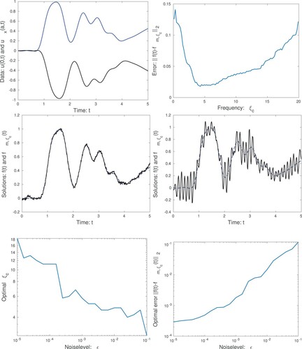
First, we set the noise level to $ϵ={10}^{-2}$ and compute an approximate surface temperature $f_{m,{\xi }_c}$, for a range of frequencies $1<{\xi }_c<20$, and compute the error $\Vert (f_{m,{\xi }_c}-f{)}_{\mathrm{\Delta }}{\Vert }_2$. The total error can be divided into two parts. First we have the truncation error $R_T=\Vert (f-f_{{\xi }_c}{)}_{\mathrm{\Delta }}{\Vert }_2$, due to the fact that not all frequencies are included in the numerical solution. Second we have the propagated data error $R_{XF}=\Vert (f_{{\xi }_c}-f_{m,{\xi }_c}{)}_{\mathrm{\Delta }}{\Vert }_2$. The stability results, see Lemmas 2.3 and  2.7, says that $R_{XF}$ is increasing as a function of ${\xi }_c$, while the truncation error $R_T$ is decreasing as a function of ${\xi }_c$. Thus the error curve has a clear minimum and an optimal ${\xi }_c$ representing the appropriate trade-off between $R_{XF}$ and $R_T$. For this case we also plot two solutions $f_{m,{\xi }_c}(t)$, for ${\xi }_c=6$ and ${\xi }_c=18$. We see that in the first case the level of regularization is just right but in the latter case there is too much noise magnification.

Next we pick noise levels in the range ${10}^{-5}\le ϵ\le {10}^{-1}$. For each level of noise we find the optimal value of ${\xi }_c$, which gives the smallest error. We see that a smaller noise ϵ means that we can use a large cut-off frequency ${\xi }_c$. We also compute the errors, for the optimal value of ${\xi }_c$, and as we expect a larger noise in the used data, leads to a larger error in the computed approximations $f_{m,{\xi }_c}(t)$.

3. Regularization by using smoothing splines

In this section we discuss the regularization of the problem (4(4) $\{\begin{array}{ll}(\kappa u_x{)}_x=u_t,& 0\le x\le a,t\ge 0,\\ u(x,0)=0,& 0\le x\le a,\\ u(a,t)=g(t),& t\ge 0,\\ u_x(a,t)=h(t)& t\ge 0,\end{array}$(4) ) using cubic smoothing splines. As previously we will implement a differentiation matrix $D_{\lambda }$ using cubic splines and solve the discretized initial value problem (10(10) ${\left(\begin{array}{c}u\\ \kappa U_x\end{array}\right)}_x=\left(\begin{array}{cc}0& {\kappa }^{-1}I\\ D& 0\end{array}\right)\left(\begin{array}{c}U\\ \kappa U_x\end{array}\right),0\le x\le a,$(10) ) numerically. The goal is to reach similar accuracy and stability properties as reported for the Fourier-based derivative $D_{{\xi }_c}$, while avoiding the practical difficulties that occur when the data vectors do not represent periodic functions.

In the following subsections we introduce a differentiation matrix $D_{\lambda }$ and also give a bound for its norm. Also we show that the matrix $D_{\lambda }$ is skew-symmetric. Thus stability results, similar to Lemmas 2.3 and  2.7, can be derived.

3.1. Differentiation using smoothing splines

In this section we present known facts about splines and introduce the notation needed in our work. For simplicity we restrict ourselves to considering the interval $0\le t\le 1$. Thus we have a uniform grid Δ, such that $0=t_1<\cdots <t_n=1$, with grid parameter h. We work in an $L^2$ setting and introduce the Sobolev space (21) $W^2[0,1]=\{u:u,u^{\mathrm{\prime }}\mathrm{abs}.\mathrm{cont}.\mathrm{on}[0,1]\mathrm{and}{u}^{\mathrm{\prime }\mathrm{\prime }}\in L^2[0,1]\},$(21) together with the standard norms and semi-norms defined, see [24].

Let $y=(y_1,y_2,\dots ,y_n{)}^T$ be a vector of data values on the grid. The smoothing cubic spline, that approximates $y_i$ on the grid, is defined as follows:

Definition 3.1

Let $y\in {\mathbb{R}}^n$ be a vector. The cubic smoothing spline $s_{\lambda }[y]$ is obtained by solving (22) $\underset{u\in W^2[0,1]}{min}h\Vert y-u_{\mathrm{\Delta }}{\Vert }_2^2+\lambda |u{|}_2^2,$(22) where $\lambda >0$ is the regularization parameter and $|u{|}_2$ denotes a semi-norm.

It is well known that the solution to (22(22) $\underset{u\in W^2[0,1]}{min}h\Vert y-u_{\mathrm{\Delta }}{\Vert }_2^2+\lambda |u{|}_2^2,$(22) ) is a natural cubic spline. It is also known that the corresponding operator, mapping $y\in {\mathbb{R}}^n$ onto $s_{\lambda }[y]\in W^2([0,1])$, is linear, see [24,25]. Thus we can introduce a matrix as follows:

Definition 3.2

The matrix $S_{\lambda }\in {\mathbb{R}}^{n\times n}$ is defined by (23) $S_{\lambda }y=(s_{\lambda }[y]{)}_{\mathrm{\Delta }}\in {\mathbb{R}}^n,\mathrm{for}\mathrm{all}y\in {\mathbb{R}}^n.$(23)

The matrix $S_{\lambda }$ has many interesting properties. For instance $\Vert S_{\lambda }{\Vert }_2\le 1$. Also, the problem (22(22) $\underset{u\in W^2[0,1]}{min}h\Vert y-u_{\mathrm{\Delta }}{\Vert }_2^2+\lambda |u{|}_2^2,$(22) ) is symmetric in the sense that $s_{\lambda }[y](t)=s_{\lambda }[\overline{y}](1-t)$, where $\overline{y}=(y_n,y_{n-1},\dots ,y_1{)}^T$ is the vector taken in reverse order. A consequence is the following result:

Lemma 3.3.

The matrix $S_{\lambda }\in {\mathbb{R}}^{n\times n}$ is symmetric.

Proof.

Let $y\in {\mathbb{R}}^n$. By introducing a basis, e.g. the B-splines $\{{\beta }_i(t){\}}_{i=0}^{n+1}$, for the space of cubic splines, and writing the minimizer of (22(22) $\underset{u\in W^2[0,1]}{min}h\Vert y-u_{\mathrm{\Delta }}{\Vert }_2^2+\lambda |u{|}_2^2,$(22) ) as $u(t)=c_0{\beta }_0(t)+\cdots +c_{n+1}{\beta }_{n+1}(t)$, we can derive an expression for $S_{\lambda }$ as follows: First $S_{\lambda }y=u_{\mathrm{\Delta }}=Ac$, where $(A{)}_{ij}={\beta }_j(t_i)$. Second, the seminorm $|u{|}_2$ can be written in the form $|u{|}_2^2=c^{T}Bc$, where $(B{)}_{ij}=({\beta }_i,{\beta }_j{)}_2$. Thus the normal equations are $(h{A}^{T}A+\lambda B)c=h{A}^{T}y$. Thus $S_{\lambda }=A(h{A}^{T}A+\lambda B{)}^{-1}{A}^T$ is symmetric. For the case $\lambda =0$, i.e. interpolating natural cubic splines, this is a known result [25].

Now we are ready to introduce the differentiation matrix $D_{\lambda }$. More precisely, we make the following definition:

Definition 3.4

The matrix $D_{\lambda }\in {\mathbb{R}}^{n\times n}$ is defined by (24) $D_{\lambda }y=(s_{\lambda }^{\prime }[y](t){)}_{\mathrm{\Delta }},\mathrm{for}\mathrm{all}y\in {\mathbb{R}}^n.$(24)

The product $D_{\lambda }y$ is computed by finding the smoothing spline $s_{\lambda }[y](t)$ and sampling its derivative on the grid.

Lemma 3.5.

The matrix $D_{\lambda }$ is skew-symmetric.

Proof.

The matrix $D_{\lambda }$ can be written in the form $D_{\lambda }=DW{A}^T$, where the matrix $W=h(h{A}^{T}A+\lambda B{)}^{-1}$ is symmetric, $(A{)}_{ij}={\beta }_j(t_i)$, and $(D{)}_{ij}={\beta }_j^{\mathrm{\prime }}(t_i)$, see the proof of Lemma 3.3. A direct calculation shows that (25) $(D_{\lambda }{)}_{i,j}=\sum _{l=0}^{n+1}\sum _{k=0}^{n+1}{\beta }_l^{\mathrm{\prime }}(t_i)w_{lk}{\beta }_k(t_j).$(25) Since the B-spline basis function ${\beta }_k(t)$ is even, with respect to $t=t_k$, and the derivative ${\beta }_l^{\mathrm{\prime }}(t)$ is odd with respect to $t=t_l$, we see that for the product ${\beta }_l^{\mathrm{\prime }}(t_i){\beta }_k(t_j)=-{\beta }_l^{\mathrm{\prime }}(t_j){\beta }_k(t_i)$. Thus we can rearrange the indices to show that $(D_{\lambda }{)}_{ij}=-(D_{\lambda }{)}_{ji}$.

A consequence of the fact that $D_{\lambda }$ is skew-symmetric is that its eigenvalues are purely imaginary. The fact is used to derive stability estimates when (10(10) ${\left(\begin{array}{c}u\\ \kappa U_x\end{array}\right)}_x=\left(\begin{array}{cc}0& {\kappa }^{-1}I\\ D& 0\end{array}\right)\left(\begin{array}{c}U\\ \kappa U_x\end{array}\right),0\le x\le a,$(10) ) is solved using the smoothing spline method.

3.2. A bound for the matrix $D_{\lambda }$

In this section we derive a bound for $\Vert D_{\lambda }{\Vert }_2$. Most of the theory presented in this section represent simplifications, with simpler proofs, of more general results found in [24], where an error estimate $|u-s_{\lambda }[u_{\mathrm{\Delta }}]{|}_1$ was derived. For our work we instead need a bound for $\Vert D_{\lambda }{\Vert }_2$ which can be obtained using similar techniques. We need a series of Lemmas.

Lemma 3.6.

Let $u\in C^{(1)}([0,1])$, $\mathrm{\Delta }=\{t_i{\}}_{i=1}^n$ be a uniform grid, and $h=t_2-t_1$. Then, if h is chosen so that $h|u{|}_1\le 0.1|u{|}_0$, it holds that (26) $c_0|u{|}_0\le \sqrt{h}\Vert u_{\mathrm{\Delta }}{\Vert }_2\le c_1|u{|}_0,$(26) where $c_0$ and $c_1$ are constants.

Proof.

We do the proof of one inequality as the other is obtained in a similar way. Let ${\nu }_i=(t_{i-1}+t_i)/2$, with ${\nu }_1=0$ and ${\nu }_{n+1}=1$. For $t,t_i\in [{\nu }_i,{\nu }_{i+1}]$ we have $\begin{array}{rl}{u}^2(t_i)& =u^2(t)+{\int }_t^{t_i}(u^2(\tau ){)}^{\mathrm{\prime }}\mathrm{d}\tau =u^2(t)+{\int }_t^{t_i}2u(\tau )u^{\mathrm{\prime }}(\tau )\mathrm{d}\tau \\ & \le u^2(t)+2{({\int }_{{\nu }_i}^{{\nu }_{i+1}}{u}^2(\tau )\mathrm{d}\tau )}^{1/2}{({\int }_{{\nu }_i}^{{\nu }_{i+1}}(u^{\mathrm{\prime }}(\tau ){)}^2\mathrm{d}\tau )}^{1/2}\end{array}$Now we can integrate over $[{\nu }_i,{\nu }_{i+1}]$, sum over all the intervals, and then use the discrete Cauchy-Schwarz inequality, to obtain (27) $h\Vert u_{\mathrm{\Delta }}{\Vert }_2^2\le |u{|}_0^2+2h|u{|}_0|u{|}_1.$(27) The result follows by using $h|u{|}_1\le 0.1|u{|}_0$. Also note that $c_1=\sqrt{1.2}$.

The above Lemma can be used to estimate the discrete norm $\Vert u_{\mathrm{\Delta }}{\Vert }_2$ in terms of the continuous norm $|u{|}_0$, and also the other way around.

In order to obtain the desired bound for $\Vert D_{\lambda }{\Vert }_2$ we need a result that follows directly from the fact that the cubic smoothing spline is the minimizer of (22(22) $\underset{u\in W^2[0,1]}{min}h\Vert y-u_{\mathrm{\Delta }}{\Vert }_2^2+\lambda |u{|}_2^2,$(22) ).

Lemma 3.7.

Let $y\in {\mathbb{R}}^n$ be a vector and $u\in W^2([0,1])$ be corresponding smoothing spline. Then (28) $h(y-u_{\mathrm{\Delta }}{)}^T{u}_{\mathrm{\Delta }}=\lambda |u{|}_2^2.$(28)

Proof.

A norm, and scalar product, for $(y,v)\in {\mathbb{R}}^n\oplus L^2([0,1])$ is given by (29) $\Vert (y,v){\Vert }^2=h\Vert y{\Vert }_2^2+\lambda |v{|}_0^2.$(29) The problem defining the cubic smoothing spline, see Lemma 3.1, can then be written as: Find $u\in W^2([0,1])$ that minimize $\Vert (y,0)-(u_{\mathrm{\Delta }},u^{\mathrm{\prime }\mathrm{\prime }})\Vert$. The solution of the least squares problem is characterized by the residual $(y-u_{\mathrm{\Delta }},-u^{\mathrm{\prime }\mathrm{\prime }})$ being orthogonal to $(v_{\mathrm{\Delta }},v^{\mathrm{\prime }\mathrm{\prime }})$, for all $v\in W^2([0,1])$. This means that (30) $h(y-u_{\mathrm{\Delta }}{)}^T{v}_{\mathrm{\Delta }}+\lambda (-u^{\mathrm{\prime }\mathrm{\prime }},v^{\mathrm{\prime }\mathrm{\prime }}{)}_0=0.$(30) Insert v = u and the result follows.

Proposition 3.8.

The matrix $D_{\lambda }$, defined by  (3.4), satisfies (31) $\Vert D_{\lambda }\Vert \le c_3{\lambda }^{-1/4},$(31) where $c_3$ is a constant.

Proof.

From the definition of $D_{\lambda }$, and using Lemma 3.6, we obtain (32) $\Vert D_{\lambda }y{\Vert }_2^2=\Vert (u^{\mathrm{\prime }}{)}_{\mathrm{\Delta }}{\Vert }_2^2\le \frac{c_1^2}{h}|u^{\mathrm{\prime }}{|}_0^2=\frac{c_1^2}{h}|u{|}_1^2,$(32) where $u(t)=s_{\lambda }[y](t)$ is the smoothing cubic spline corresponding to the vector $y\in {\mathbb{R}}^n$. Next we use the inequality (33) ${\tau }^2|u{|}_1^2\le c_2(|u{|}_0^2+{\tau }^4|u{|}_2^2),$(33) where $c_2$ is a constant, which is valid for $0<\tau <1$, and all $u\in W^2([0,1])$, see [24, Lemma 3.9] or, originally, [26]. We obtain (34) $\Vert D_{\lambda }y{\Vert }_2^2\le \frac{c_1^2{c}_2}{h{\tau }^2}(|u{|}_0^2+{\tau }^4|u{|}_2^2)\le \frac{c_1^2{c}_2}{h{\tau }^2}(\frac{h}{c_0^2}\Vert u_{\mathrm{\Delta }}{\Vert }_2^2+{\tau }^4|u{|}_2^2),$(34) where we again used Lemma 3.6. For the final step we write $y=y-u_{\mathrm{\Delta }}+u_{\mathrm{\Delta }}$ and expand $\Vert y{\Vert }_2^2$ into (35) $\Vert y{\Vert }_2^2=(y-u_{\mathrm{\Delta }}+u_{\mathrm{\Delta }}{)}^T(y-u_{\mathrm{\Delta }}+u_{\mathrm{\Delta }})=\Vert y-u_{\mathrm{\Delta }}{\Vert }_2^2+2(y-u_{\mathrm{\Delta }}{)}^T{u}_{\mathrm{\Delta }}+\Vert u_{\mathrm{\Delta }}{\Vert }_2^2.$(35) By inserting Lemma 3.7 into the above expression we obtain (36) $\Vert y{\Vert }_2^2=\Vert y-u_{\mathrm{\Delta }}{\Vert }_2^2+\frac{2\lambda }{h}|u{|}_2^2+\Vert u_{\mathrm{\Delta }}{\Vert }_2^2.$(36) From (36(36) $\Vert y{\Vert }_2^2=\Vert y-u_{\mathrm{\Delta }}{\Vert }_2^2+\frac{2\lambda }{h}|u{|}_2^2+\Vert u_{\mathrm{\Delta }}{\Vert }_2^2.$(36) ) we obtain the two estimates (37) $|u{|}_2^2\le \frac{h}{2\lambda }\Vert y{\Vert }_2^2,\mathrm{and}\Vert u_{\mathrm{\Delta }}{\Vert }_2^2\le \Vert y{\Vert }_2^2.$(37) Inserting these two inequalities into (34(34) $\Vert D_{\lambda }y{\Vert }_2^2\le \frac{c_1^2{c}_2}{h{\tau }^2}(|u{|}_0^2+{\tau }^4|u{|}_2^2)\le \frac{c_1^2{c}_2}{h{\tau }^2}(\frac{h}{c_0^2}\Vert u_{\mathrm{\Delta }}{\Vert }_2^2+{\tau }^4|u{|}_2^2),$(34) ) yields (38) $\Vert D_{\lambda }y{\Vert }_2^2\le \frac{c_1^2{c}_2}{h{\tau }^2}(\frac{h}{c_0^2}+\frac{{\tau }^{4}h}{2\lambda })\Vert y{\Vert }_2^2.$(38) The result follows by inserting $\tau ={\lambda }^{1/4}$ into (38(38) $\Vert D_{\lambda }y{\Vert }_2^2\le \frac{c_1^2{c}_2}{h{\tau }^2}(\frac{h}{c_0^2}+\frac{{\tau }^{4}h}{2\lambda })\Vert y{\Vert }_2^2.$(38) ).

3.3. Stability analysis for cubic splines

In this section we establish stability results, for the initial value problem (10(10) ${\left(\begin{array}{c}u\\ \kappa U_x\end{array}\right)}_x=\left(\begin{array}{cc}0& {\kappa }^{-1}I\\ D& 0\end{array}\right)\left(\begin{array}{c}U\\ \kappa U_x\end{array}\right),0\le x\le a,$(10) ), when the approximation ${\mathrm{\partial }}_t\approx D=D_{\lambda }$ is used. The proofs are based on the idea that since $D_{\lambda }$ is skew-symmetric we have an eigenvalue decomposition (39) $D_{\lambda }=X{\mathrm{\Lambda }}_{\lambda }{X}^H,({\mathrm{\Lambda }}_{\lambda }{)}_{j,j}=i{\lambda }_j,$(39) where the eigenvector matrix X is unitary, the ${\lambda }_j$ are real, and are bounded by $|{\lambda }_j|\le c_3{\lambda }^{-1/4}/b$. The factor b is due to the fact that the theory in the previous section was developed under the assumption that the time interval was 0<t<1.

Lemma 3.9.

Let $D=D_{\lambda }$, where $\lambda >0$ is the regularization parameter, and let $U_1$ and $U_2$ be two different solutions to  (10(10) ${\left(\begin{array}{c}u\\ \kappa U_x\end{array}\right)}_x=\left(\begin{array}{cc}0& {\kappa }^{-1}I\\ D& 0\end{array}\right)\left(\begin{array}{c}U\\ \kappa U_x\end{array}\right),0\le x\le a,$(10) ), corresponding to Cauchy data $[(g_1{)}_{\mathrm{\Delta }},h_{\mathrm{\Delta }}]$ and $[(g_2{)}_{\mathrm{\Delta }},h_{\mathrm{\Delta }}]$, respectively. Then (40) $\Vert U_1(x)-U_2(x){\Vert }_2\le \cosh (\sqrt{\sigma }(a-x))\Vert (g_1-g_2{)}_{\mathrm{\Delta }}{\Vert }_2,\sigma =\frac{c_3{\lambda }^{-1/4}}{2b\kappa }.$(40)

Proof.

Let X be as defined in (39(39) $D_{\lambda }=X{\mathrm{\Lambda }}_{\lambda }{X}^H,({\mathrm{\Lambda }}_{\lambda }{)}_{j,j}=i{\lambda }_j,$(39) ) and introduce a new variable $V=X^H(U_1-U_2)$. The system (10(10) ${\left(\begin{array}{c}u\\ \kappa U_x\end{array}\right)}_x=\left(\begin{array}{cc}0& {\kappa }^{-1}I\\ D& 0\end{array}\right)\left(\begin{array}{c}U\\ \kappa U_x\end{array}\right),0\le x\le a,$(10) ) simplifies to (41) $\kappa V_{xx}={\mathrm{\Lambda }}_{\lambda }V,0<x<a,$(41) with boundary conditions $V(a)=X^H(g_1-g_2{)}_{\mathrm{\Delta }}$ and $V_x(a)=X^H(h-h{)}_{\mathrm{\Delta }}=0$. This is exactly the same situation as in the proof of Lemma 2.3 and the result follows by repeating the same steps.

Similarily we can repeat the steps for the proof of Lemma 2.7 to obtain the following result:

Lemma 3.10.

Let $D=D_{{\xi }_c}$, where $\lambda >0$ is the regularization parameter, and let $U_1$ and $U_2$ be two different solutions to  (10(10) ${\left(\begin{array}{c}u\\ \kappa U_x\end{array}\right)}_x=\left(\begin{array}{cc}0& {\kappa }^{-1}I\\ D& 0\end{array}\right)\left(\begin{array}{c}U\\ \kappa U_x\end{array}\right),0\le x\le a,$(10) ), corresponding to Cauchy data $[g_{\mathrm{\Delta }},(h_1{)}_{\mathrm{\Delta }}]$ and $[g_{\mathrm{\Delta }},(h_2{)}_{\mathrm{\Delta }}]$. Then (42) $\Vert U_1(x)-U_2(x){\Vert }_2\le \frac{\sinh (\sqrt{\sigma }(a-x))+1}{\sqrt{\sigma }}\Vert (h_1-h_2{)}_{\mathrm{\Delta }}{\Vert }_2,\sigma =\frac{c_3{\lambda }^{-1/4}}{2b\kappa }.$(42)

The above results means that the problem (10(10) ${\left(\begin{array}{c}u\\ \kappa U_x\end{array}\right)}_x=\left(\begin{array}{cc}0& {\kappa }^{-1}I\\ D& 0\end{array}\right)\left(\begin{array}{c}U\\ \kappa U_x\end{array}\right),0\le x\le a,$(10) ) is well-posed when the approximation ${\mathrm{\partial }}_t\approx D_{\lambda }$ is used. The regularization parameter λ fills the same role as the cut-off frequency ${\xi }_c$ for the Fourier method. For this method a small value for λ leads to a more accurate derivative and thus less stability for the inverse problem. If ${\xi }_c\approx {\lambda }^{-1/4}$ then both methods satisfy similar stability estimates.

4. Simulated numerical examples

In this section we present numerical examples intended to illustrate the properties of the smoothing spline method. The experiments are constructed essentially the same way as in Section 2.4. There are many codes available for solving the minimization problem (22(22) $\underset{u\in W^2[0,1]}{min}h\Vert y-u_{\mathrm{\Delta }}{\Vert }_2^2+\lambda |u{|}_2^2,$(22) ) and for our work we use the Matlab function csaps; which can be used to find the cubic smoothing spline $s_{\lambda }[y](t)$ for a given vector y, a stepsize h, and regularization parameter λ .¹

Test 1 As a first experiment we solve the same problem, as was used in Section 2.4. Thus we first set the noise level to be $ϵ={10}^{-2}$ and solve the inverse problem for a wide range of regularization parameters λ. In Figure 3 we present the results. We note that, as previously, there is an optimal regularization parameter λ, which represents the appropriate trade-off between accuracy and stability. We also display the computed solution for $\lambda =2\cdot {10}^{-8}$ which is close to the optimal value. The accuracy of the numerical solution is comparable to that computed by the Fourier method.

Figure 3. In the top-left graph we show the error $\Vert f_{m,\lambda }-f{\Vert }_2$, as a function of λ, for the noise level $ϵ={10}^{-2}$. Note that there is an optimal value for λ. In the top-right graph we display the surface temperature for $\lambda =2\cdot {10}^{-8}$ which is close to the optimal value. In the bottom-left graph we show the optimal λ as a function of the noise level ϵ and in the bottom-right graph we show the corresponding error, for the optimal λ, as a function of ϵ. Note that for a larger noise level ϵ, we need a larger value of λ, and obtain a larger error in the computed surface temperature $f_{m,\lambda }(t)$.

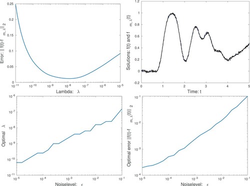
Next we illustrate the regularization properties of the method by letting the noise level vary in the range ${10}^{-5}\le ϵ\le {10}^{-1}$. For each different noise level we find the optimal λ and compute the corresponding error. smallest error. We see that a smaller noise ϵ means that we can use a smaller λ, and thus compute the derivatives more accurately. We also see that a larger noise in the data leads to a larger error in the computed surface temperatures $f_{m,\lambda }(t)$. The results are comparable to those reported in Section 2.4.

Test 2 In order to further investigate the properties of the two numerical methods we select a variable coefficient (43) $\kappa (u)=1+\sin (\pi u{)}^{0.8}+4.2\exp (-27.3(a/3-u{)}^2).$(43) This choice of $\kappa (u)$ gives a slightly less ill-posed problem compared to our previous test. Note that since the problem now is non-linear iteration is needed to solve the problem and create numerical test data. The numerical code for the inverse problem (10(10) ${\left(\begin{array}{c}u\\ \kappa U_x\end{array}\right)}_x=\left(\begin{array}{cc}0& {\kappa }^{-1}I\\ D& 0\end{array}\right)\left(\begin{array}{c}U\\ \kappa U_x\end{array}\right),0\le x\le a,$(10) ) remains the same. For this experiment we chose a smoothed out stepfunction $f(t)$ as the exact surface temperature and the time interval is 0<t<b, where b = 5. The size of the time grid is again n = 400. Our objective is to try and verify that the Fourier transform method leads to a larger error, at the beginning of the time interval due to the implicit periodicity assumption. This motivates our choice of $f(t)$ as a step function. The idea is that Gibbs phenomena near the discontinuity causes a larger error in the second half of the interval $[0,b]$, and that this should also cause errors near t = 0 for the Fourier method. We use a smoothed out step function, and not a true discontinuity, to make the test a bit easier for the Fourier method.

First we compute the errors $\Vert f-f_{m,\lambda }{\Vert }_2$ and $\Vert f-f_{m,{\xi }_c}{\Vert }_2$ for a range of regularization parameters. For this test we use the noise level $ϵ={10}^{-2}$. The results are displayed in Figure 4. We see that for both methods too little regularization leads to a large error due to instability. However, also for both methods, the truncation error is fairly large due to Gibbs phenomena regardless of the choice of the regularization parameter. There is no clear optimal choice for the level of regularization. We also display two approximate solutions for $\lambda ={10}^{-8}$ and ${\xi }_c=7$, respectively. Both solutions are about as accurate however the spline method clearly leads to a smaller error initially. This is due to a lack of wrap-around effects.

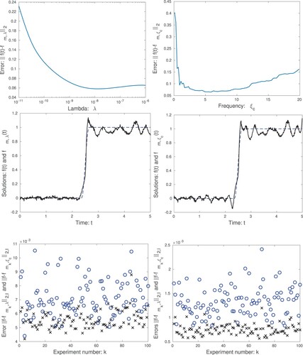
Figure 4. We present tests where the exact solution $f(t)$ is a smoothed step function. The top graphs show the error $\Vert f-f_{m,\lambda }{\Vert }_2$ (left) for the spline method and the error $\Vert f-f_{m,{\xi }_c}{\Vert }_2$ (right) for the Fourier method. The middle graphs display the numerical solutions $f_{m,\lambda }(t)$ (left) obtained using the spline method and $\lambda ={10}^{-8}$ and the solution $f_{m,{\xi }_c}(t)$ computed using the Fourier method and ${\xi }_c=7$. The lower graphs show the errors $\Vert f-f_{m_k,\lambda }{\Vert }_2$ x markers) and $\Vert f-f_{m_k,{\xi }_c}{\Vert }_2$ o markers) for different random noise sequences ${ϵ}_k$. In the left graph the variance of the noise is $ϵ={10}^{-2}$, $\lambda ={10}^{-8}$ and ${\xi }_c=7$. In the right graph instead $ϵ={10}^{-3}$, $\lambda =2\cdot {10}^{-9}$ and ${\xi }_c=8.3$. In both cases 100 different sets of random noise were generated.

The noise level $ϵ={10}^{-2}$ represents the variance of the normally distributed random noise added to the data $[g_{\mathrm{\Delta }},h_{\mathrm{\Delta }}]$ at individual grid points. However an observation is that different random sequences can give quite different errors in the computed solutions. Thus we perform 100 different experiments, with the same parameters b = 5, $ϵ={10}^{-2}$ and $\kappa (x)$ as specified above. For each experiment we compute the error using the Euclidea norm $\Vert \cdot {\Vert }_{2,I}$, where only grid points $t_i$ inside the interval $I=[0,1]$ counts towards the sum. This means that we only look at the errors at the beginning of the time interval.

To select the appropriate levels of regularization is difficult since the methods behave differently. In this case we did the following: We use the exact solution $f(t)=0$, and thus $g_{\mathrm{\Delta }}=h_{\mathrm{\Delta }}=0$. This means we only have noise. We picked $\lambda ={10}^{-8}$ and adjusted ${\xi }_c$ until both methods give the same mean error, over 100 tests. In this case that happens for ${\xi }_c\approx 7$. Thus the parameters are chosen so that random noise is magnified equally by both methods. The results are shown in Figure 4. We see that for the step function $f(t)$ the error, measured using $\Vert \cdot {\Vert }_{2,[0,1]}$, is on average significantly larger for the Fourier method which shows that the method suffers from problems with wrap-around effects.

We also tried a lower noise level $ϵ={10}^{-3}$. In this case the appropriate regularization parameters are $\lambda =2\cdot {10}^{-9}$ and ${\xi }_c=8.3$. Again when we run 100 tests, with different noise sequences, we see that the spline method has a smaller error initially, due to avoidance of wrap-around effects.

5. Concluding remarks

In this paper we have developed a regularization method for solving the inverse heat conduction problem by using smoothing cubic splines. Previously, the same problem has been solved using Fourier transforms [2,7,13]. The Fourier method is working well but makes the implicit assumption that the data vectors represents periodic functions. This is not true for the problem under consideration and this can potentially lead to very large errors in practice. We present one of the standard techniques, called periodization, that is used to deal with non-periodic data vectors and thus avoid wrap-around effects. In our work we show that, while the periodization works reasonably well, there are increased errors in the numerical solution due to the periodicity assumptions needed for the Fourier method. To avoid the need for a periodicity assumption is why we introduce the smoothing spline method as an alternative. Our experiments show that we do indeed avoid an increased error due to wrap-around effects.

The inverse heat conduction problem is ill-posed in the sense that small errors in the data can cause large errors in the numerical solution. Thus regularization is needed. We demonstrate that the Fourier method is a regularization of the problem by providing stability estimates. The stability theory is developed for the discrete problem that is solved numerically. Though a complication is that the periodization procedure is not included in the stability analysis.

For the smoothing spline method we introduce a matrix $D_{\lambda }$ that represents differentiation of the smoothing spline obtained from a vector y consisting of function values on the grid. Our goal is to develop similar stability estimates as for the Fourier method. Thus we derive a bound on the norm $\Vert D_{\lambda }{\Vert }_2$ and also show that the matrix is skew-symmetric. Our theory is based on a previous paper [24] but since our work concerns only a special case we can obtain simpler proofs. Since no periodicity assumption is needed, as for the Fourier method, one advantage is that the stability theory corresponds more directly to the discrete problem that is actually solved by our codes. From our experiments we also deduce that the smoothing splines method can effectively be used as a regularization method for solving the Cauchy problem.

In this paper we only present a stability analysis that bounds the errors in the solution caused by random errors in the data. In [24] an error estimate $\Vert u^{\mathrm{\prime }}-s_{\lambda }^{\mathrm{\prime }}[u_{\mathrm{\Delta }}]{\Vert }_{L^2}$ is derived. In future work we intend to make use of a similar error estimate for our matrix approximation $D_{\lambda }$ and also limit the truncation error for our method. We also intend to apply our method to similar problems and compare with the work of other authors, e.g. [16,18]. We are also looking to apply the method to industrial problems with measured data.

Acknowledgments

The work of Mary Nanfuka is supported by the SIDA bilateral programme (2015–2020) with Makerere University; Project 316: Capacity building in Mathematics. The authors also thank prof. Matti Heiliö for valuable discussions during the work.

Disclosure statement

No potential conflict of interest was reported by the author(s).

Notes

1 The code used for our experiments is made available upon request by the corresponding author

References

- Beck JV, Blackwell B, Clair SR. Inverse heat conduction. Ill-posed problems. New York: Wiley; 1985.
- Eldén L, Berntsson F, Regińska T. Wavelet and Fourier methods for solving the sideways heat equation. SIAM J Sci Comput. 2000;21(6):2187–2205.
- Gardarein J-L, Gaspar J, Corre Y, et al. Inverse heat conduction problem using thermocouple deconvolution application to the heat flux estimation in a tokamak. Inverse Probl Sci Eng. 2013;21(5):854–864.
- Jahedi M, Berntsson F, Wren J, et al. Transient inverse heat conduction problem of quenching a hollow cylinder by one row of water jets. Int J Heat Mass Transf. 2018;117(Supplement C):748–756.
- Li D, Wells MA. Effect of subsurface thermocouple installation on the discrepancy of the measured thermal history and predicted surface heat flux during a quench operation. Metallurg Mater Trans. 2005;36B:343–354.
- Taler J, Weglowski B, Pilarczyk M. Monitoring of thermal stresses in pressure components using inverse heat conduction methods. Int J Numer Meth Heat Fluid Flow. 2017;27(3):740–756.
- Wikström P, Blasiak W, Berntsson F. Estimation of the transient surface temperature, heat flux and effective heat transfer coefficient of a slab in an industrial reheating furnace by using an inverse method. Steel Res Int. 2007;78(1):63–70.
- Berntsson F. An inverse heat conduction problem and improving shielded thermocouple accuracy. Numer Heat Transfer, Part A: Appl. 2012;61(10):754–763.
- Xiong X-T, Fu C-L. A spectral regularization method for solving surface heat flux on a general sideways parabolic. Appl Math Comput. 2008;197(1):358–365.
- Carasso AS. Slowly divergent space marching schemes in the inverse heat conduction problem. Numer Heat Transfer, Part B. 1993;23:111–126.
- Guo L, Murio DA, Roth C. A mollified space marching finite differences algorithm for the inverse heat conduction problem with slab symmetry. Computers Math Appl. 1990;19:75–89.
- Mejía CE, Murio DA. Numerical solution of generalized IHCP by discrete mollification. Computers Math Appl. 1996;32:33–50.
- Berntsson F. A spectral method for solving the sideways heat equation. Inverse Probl. 1999;15:891–906.
- Blevins LG, Pitts WM. Modeling of bare and a spirated thermocouples in compartment fires. Fire Saf J. 1999;33:239–259.
- Kemp SE, Annaheim S, Rossi RM, et al. Test method for characterising the thermal protective performance of fabrics exposed to flammable liquid fires. Fire Mater. 2016;41:750–767.
- Karimi M, Rezaee A. Regularization of the Cauchy problem for the Helmholtz equation by using Meyer wavelet. J Comput Appl Math. 2017;320:76–95.
- Regińska T. Sideways heat equation and wavelets. J Comput Appl Math. 1995;63:209–214.
- Foadian S, Pourgholi R, Hashem Tabasi S. Cubic b-spline method for the solution of an inverse parabolic system. Appl Anal. 2018;97(3):438–465.
- Reinsch CH. Smoothing by spline functions. Numer Math. 1971;16(5):451–454.
- Isakov V. Inverse problems for partial differential equations. New York: Springer; 1998.
- Eldén L. Solving the sideways heat equation by a ‘method of lines’. J Heat Transfer, Trans ASME. 1997;119:406–412.
- Gustafsson B, Kreiss H-O, Oliger J. Time dependent problems and difference methods. New York: Wiley Interscience; 1995.
- Anderson GD, Vamanamurthy MK, Vuorinen MK. Conformal invariants, inequalities, and quasiconformal maps. New York: John Wiley & Sons, Inc.; 1997.
- Ragozin DL. Error bounds for derivative estimates based on spline smoothing of exact or noisy data. J Approx Theor. 1983;37(4):335–355.
- Schoenberg IJ. Spline interpolation and the higher derivatives. Proc Nat Acad Sci USA. 1964;51:24–28.
- Agmon S. Lectures on elliptic boundary value problems. Princeton (NJ): D. Van Nostrand Co.; 1965.