Export margins and world shocks: an empirical investigation in fixed and floating regimes

ABSTRACT

We use 4-digit data to document the role of world shocks for intensive and extensive margin of exports. We estimate a VAR model, where the endogenous bloc comprises bilateral export margins and relative GDP, and the exogenous bloc comprises disaggregated measures of world price shocks. We find that world shocks have a significant impact on both the average export volume and export diversification. Impulse responses display considerable heterogeneity depending on the shock considered, the exchange rate regime and the great trade collapse. The evidence in the paper has remarkable consequences for trade and exchange rate policies.

KEYWORDS:

• Exports
• export margins
• exchange rate regimes
• vector autoregressions (VAR)
• world shocks

JEL CLASSIFICATION:

• E31
• E32
• E52
• F10
• F14

I. Introduction

This paper investigates the role of world prices in an empirical model by examining the effect of shocks to key international prices on the extensive and intensive export margins. Trade expansion can be decomposed into an increase in the average exports by firms that are already exporters (the firm-level intensive margin) and the number of exporters selling in the destination market (the firm-level extensive margin). When firms produce differentiated products, these firm-level margins map into product-level margins, which are the object of our empirical study. The extensive margin is the (eventually weighted) number of products exported and provides a measure of export diversification. The intensive margin is the average volume of exports per product and is a measure of export size.

The importance of world shocks in the international real business cycle has long been recognized, and shocks transmitted by fluctuations in key international prices represent a major source of variations for output and other aggregate indicators (Mendoza 1995; Kose 2002). Shocks that depreciate a country’s terms of trade (the price of exports relative to the price of imports) reduce output, and the impact is typically high in developing countries and small open economies, and for countries in fixed regimes (Broda 2004). Moreover, terms of trade shocks affect trade mainly at the extensive margin, and particularly so in fixed regimes (Cavallari and D’Addona 2015). Recent empirical work based on vector autoregressions suggests that single measures of world prices – like the terms of trade – can explain only a small portion of variations in trade and aggregate indicators in poor and emerging countries (Schmitt-Grohé and Uribe 2018) as well as in developed and developing countries (Fernández, Schmitt-Grohé, and Uribe 2017). These studies recommend the use of more disaggregated world price measures for studying trade and macroeconomic dynamics.

Recent developments at the intersection between trade and macroeconomics have pointed out that firms’ selection into export markets is key to understand the way shocks are transmitted in the world economy: models with entry and exit of exporters (the extensive margin) predict larger and more persistent output effects compared to models in which shocks are transmitted only by fluctuations in the average amount of export per firm (the intensive margin).¹ Moreover, trade at the extensive margin helps to reconcile the predictions of standard international real business cycle models with the comovements of macroeconomic aggregates observed in the data (Cavallari 2013). These studies argue that variations at the extensive and intensive margins can have different implications for aggregate variables and suggest decomposing trade into these margins in the formulation of empirical and theoretical open economy models.

Accordingly, this paper presents an empirical model of trade in which multiple world prices transmit the effects of global shocks to the extensive and intensive margins of bilateral exports. Specifically, it estimates a structural panel VAR model with a country-pair bloc and an exogenous world bloc, VAR-X for short. The country-pair bloc includes intensive and extensive margins of bilateral exports, together with relative GDP. The world bloc, which is common to all country-pairs, includes three commodity prices (agricultural, metal and fuel prices) and the world interest rate as in Fernández, Schmitt-Grohé, and Uribe (2017). The VAR-X is estimated for 22 OECD economies over the period 1988 to 2018.

We document a significant impact of world prices on export margins. Shocks to agricultural and metal prices, and shocks to interest rates are associated with a drop in the average volume of exports, reflecting a contraction in world demand. Shocks to fuel prices, on the contrary, increase average export volumes, capturing a boost in world supply. All shocks, except interest rates, have a substantial impact on export diversification.

Interestingly, we find substantial differences in the dynamics of the model depending on the exchange rate regime and the great trade collapse. Exchange rate flexibility appears to facilitate adjustment at the intensive margin, while pegging the domestic currency may facilitate adjustment at the extensive margin. These effects are particularly strong for interest rate shocks. We document a considerable and persistent increase in the impact of all shocks after the great trade collapse.

The rest of the paper is organized as follows. Section 2 displays some regularities in the data. Section 3 presents the empirical strategy. Section 4 discusses the results, Section 5 provides a robustness analysis, and Section 6 concludes.

II. The data

We use a panel of four world prices (three commodity prices and a world interest rate) and three aggregate indicators (extensive and intensive export margins, and relative output) measured on a country-pair basis among 22 OECD economies.² The sample is annual and covers the period 1988 to 2018.

Macroeconomic data come from the OECD’s Statextract. GDP is measured in constant, national currency units and is deflated using the national Consumer Price Index. The world interest rate is proxied by the real three-month U.S. Treasury bill rate from the FRED II Database provided by the Fedaral reserve Bank of St. Louis. The real Treasury bill rate is obtained by subtracting the U.S. CPI inflation rate over the previous 12 months from the annualized Treasury bill rate, then the annual rate is computed taking the arithmetic average of the monthly rates for each year.

Data on commodity prices come from the World Bank Commodity Price Data (The Pink Sheet). We focus on the commodity price indices for Fuels, Agriculture, and Metals. These indices are expressed in terms of a composite good, comprising all other goods, whose price is proxied by the U.S. Consumer Price Index. The annual time series are averages of the monthly data over the 12 months of a year.

Trade data come from the United Nations’ Commodity Trade database (COMTRADE), which is publicly accessible through the World Bank’s World Integrated Trade Solution³ We work with bilateral trade flows at the product level, where product category is defined according to the United Nations’ four-digit Standard International Trade Classification⁴ The unit of observation is the triad $X_{j,m,i}$ representing exports from country $j$ to country $m$ of product $i$. We restrict our analysis to OECD countries, ignoring small countries to avoid zero bilateral trade flows and to ensure sufficient overlap in SITC4 products across importer-exporter pairs.

We follow Hummels and Klenow (2005), HK, in decomposing trade flows into an extensive and an intensive margin. The extensive margin represents new export lines: it is given by a count of products exported to a given destination, eventually weighted by their share in world trade. Weigths are meant to capture the expansion potential of a new export line, so starting to export a product which is important in world trade counts more than starting to export a product which is less important in world trade. We construct both the HK measure and the simple measure in Eaton and Fieler (2019).

The HK measure weights new exports by their share in world trade. Specifically, let $I_{jm}$ be the set of products exported by country $j$ to country $m$, $X_{m,i}^W$ the dollar value of world’s exports of product $i$ to country $m$, and $X_m^W$ the dollar value of aggregate world’s exports to country $m$, then the extensive margin of exports from country $j$ to country $m$ is:

(1) $X{M}_{jm}=\frac{{\sum }_{i\in I_{jm}}{X}_{m,i}^W}{X_m^W}$(1)

The simple measure of the extensive margin is given by the fraction of products that $j$ exports to $m$ relative to all products exported to $m$:

(2) $X{M}_{jm}=\frac{{\sum }_{i\in I_{jm}}i}{{\sum }_{i\in I_{Wm}}i}$(2)

where $I_{Wm}$ is the set of products that the world export to $m$. This measure, constructed as a count of exported products that is independent of export value, is convenient in data sets spanning a large number of countries and long periods of time. We consider the simple measure for robustness purposes.

The intensive margin reflects the size of a country’s exports to a given destination. It is defined as follows:

(3) $I{M}_{jm}=\frac{{\sum }_{i\in I_{jm}}{X}_{j,i}}{{\sum }_{i\in I_{jm}}{X}_{m,i}^W}$(3)

where $X_{j,i}$ is the dollar value of $j$’s exports of product $i$ to country $m$. In words, the numerator is $j$’s aggregate exports to country $m$ and the denominator is world exports to country $m$ of products that are in $j$’s export portfolio. That is, the intensive margin is $j$’s market share in what it exports to country $m$.

By construction, all these measures are between zero and one. Notice that the categories of goods exported might differ across exporters and change over time. The measurement implies that a country would have a higher extensive margin if it exports many different categories of products to a given destination, whereas, it would have a higher intensive margin if it exports only few categories to this destination. Hence, the extensive margin increases with the number of products exported and is a measure of export diversification. The intensive margin increases with the volume of exports per product and is a measure of export size.

Extensive and intensive margins of bilateral exports

We start by describing some regularities of the data. Figures 1 and 2 report the median, the 25${ }^{th}$ and 75${ }^{th}$ percentiles of, respectively, the HK intensive and extensive margins from each country towards all destinations. Table 1 reports the volatility of these margins, and the correlation with output in the origin and destination countries. In appendix A.1, we provide comparable statistics using the simple measure.

Table 1. Summary statistics.

	σxm	σim	σxm/σim	ρ(xm, ∆gpdh)	ρ(xm, ∆gpdf)	ρ(im, ∆gpdh)	ρ(im, ∆gpdf)
Australia	0.239	0.065	3.686	0.018	0.022	−0.008	0.085
Belgium	0.056	0.068	0.822	−0.005	−0.019	0.007	0.025
Canada	0.118	0.042	2.813	−0.113	−0.040	−0.059	0.058
Switzerland	0.067	0.028	2.408	0.029	−0.034	0.109	−0.034
Czech Republic	0.155	0.009	17.633	0.058	−0.202	−0.020	−0.195
Germany	0.043	0.143	0.298	0.050	0.132	0.234	−0.036
Spain	0.082	0.064	1.267	0.025	−0.068	0.027	−0.092
Finland	0.114	0.021	5.330	0.043	−0.099	0.031	−0.033
France	0.046	0.046	0.992	0.053	−0.063	0.104	−0.052
United Kingdom	0.038	0.042	0.915	0.050	−0.020	0.150	0.048
Iceland	0.208	0.018	11.261	0.097	−0.197	−0.091	0.110
Italy	0.050	0.030	1.679	0.013	−0.057	0.126	−0.062
Japan	0.133	0.101	1.325	0.116	0.087	0.383	0.285
Korea Rep.	0.156	0.030	5.266	−0.077	−0.028	0.187	0.103
Luxembourg	0.222	0.002	128.841	−0.018	−0.168	0.075	−0.020
Mexico	0.264	0.029	9.145	−0.026	−0.130	0.004	0.012
Netherlands	0.049	0.034	1.438	0.013	−0.008	−0.066	−0.186
Norway	0.157	0.022	7.144	−0.036	−0.120	0.001	−0.022
New Zealand	0.262	0.013	20.860	0.008	−0.053	−0.092	0.120
Portugal	0.194	0.016	11.800	−0.100	−0.169	0.216	−0.078
Sweden	0.060	0.050	1.194	0.056	−0.026	−0.025	−0.007
United States	0.054	0.182	0.295	0.146	0.127	0.040	0.077
Mean	0.126	0.048	10.746	0.018	−0.052	0.061	0.005
Standard deviation	0.078	0.044	26.994	0.064	0.093	0.119	0.106

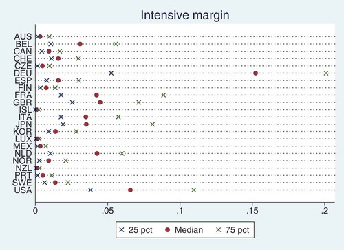
The intensive margin of each country is the average market share of that country in the portfolio of products that it exports to all destinations in the sample. Intensive margins measured by market shares have typically a small range of variation, between zero and 0.15 in our data. In small countries, the median value is close to the lower end of this spectrum, reflecting an export pattern skewed towards a relatively small size. Large, manufacturing countries, on the contrary, display median values close to the middle of the distribution.

Figure 1. Distribution of intensive margins.

This figure displays the median, the ${25}^{th}$ and the ${75}^{th}$ percentile of intensive margins for all the countries in the sample.

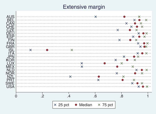
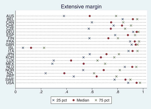
The extensive margin of each country is a measure of the average degree of diversification of that country’s exports towards all destinations. It has a much larger range of variation compared to the intensive margin. For most countries the distribution is skewed towards the higher end of this range, reflecting a tendency to diversify exports across destinations. Not surprisingly, large countries appear to diversify more than small countries. Iceland is the country with the lowest score. This, together with a high market share, speaks of a high degree of specialization in Icelandic exports.

Figure 2. Distribution of extensive margins.

This figure displays the median, the 25^th and the 75^th percentile of extensive margins for all the countries in the sample.

Two conclusions can be drawn from Table 1. First, the extensive margin of exports is fairly volatile, and far more volatile than the intensive margin: the standard deviation of the extensive margin is more than 10 times larger than that of the intensive margin on average. Volatility is particularly high in small economies. A high volatility of the extensive margin is in line with evidence in Naknoi (2015), stressing that the extensive margins of exports to and from the United States are more volatile than output in the exporting and importing country on average. Second, the extensive margin appears to be almost uncorrelated with output in the origin and destination country on average. The United States are an exception, with a positive correlation of, respectively, 0.146 and 0.127. The intensive margin is also very weakly and positively correlated with domestic and foreign output. Overall, these facts suggest that the categories of products that are exported in the world economy vary substantially over the business cycle, and they do so far more than the volume of exports per product. These fluctuations may be driven by local and global shocks. The analysis of the role of world shocks is the focus of the rest of the paper.

III. Empirical specification

We model a panel VAR with a vector of exogenous variables (VAR-X for short). The model includes three endogenous variables and four exogenous variables. Endogenous variables are measured on a country-pair basis where $j=1,2,...22$ denotes the exporting country, $m=1,2,...22$ with $m\ne j$ denotes the destination country, and $t$ indicates time. Endogenous include relative GDP and bilateral exports, measured at the extensive and the intensive margin. Relative output controls for country’s size in the tradition of gravity models. The exogenous vector represents shocks to world prices that do not depend on the dynamics of any of the endogenous variables. It is common to all panels and comprises innovations to agricultural prices $P^a$, fuel prices $P^f$, metal prices $P^m$ and the world interest rate $r$. The latter is measured by the real three-month U.S. Treasury bill rate.

First, we estimate world shocks following Fernández, Schmitt-Grohé, and Uribe (2017). Let $p_t$ $=(P^a,$ $P^m,$ $P^f,$ $r_t)$ be the vector of world prices. We assume that it evolves according to the following first-order autoregressive system:

(4) $p_t=A{p}_{t-1}+e_t$(4)

where $A$ is a matrix of coefficients, and $e_t$ is an i.i.d. mean-zero random vector with variance-covariance matrix $E(e_t{e}_t^{\prime })=\mathrm{\Sigma }$ . The system (4) is estimated by ordinary least squares (OLS) equation by equation. Structural shocks are identified recursively by a Cholesky decomposition, where the ordering of variables in vector $p_t$ reflects the degree of endogeneity. The interest rate is assumed to react to changes in all prices and is therefore ordered last. Fuel prices are assumed to affect other prices and are ordered third. We do not have any particular reason for ordering the remaining prices and consider alternative identifications with agricultural prices or metal prices in first position.⁵

Then, we estimate the VAR-X model:

(5) $Y_{j\times m,t}={\alpha }_{j\times m}+\beta (L)Y_{j\times m,t-1}+\gamma (L)X_t+{\epsilon }_{j\times m,t}$(5)

where $Y_{j\times m,t}=(\frac{GD{P}_{j,t}}{GD{P}_{m,t}},$ $X{M}_{jxm,t},$ $I{M}_{j\times m,t})$ is the vector of endogenous variables; ${\alpha }_{j\times m}$ captures country-pair fixed effects; $\beta (L)$ and $\gamma (L)$ are matrix polynomials in the lag operator, ${\epsilon }_{j\times m,t}$ is the vector of errors in the system, and $X_t$ is the vector of world shocks obtained from the first step. Notice that these shocks are by construction orthogonal to any of the endogenous variables in the system and can be treated as exogenous in (5).

We estimate the model (5) using the bootstrap bias-corrected estimator (BSBC) in Pesaran and Zhao (1999) and Everaert and Pozzi (2007). The bootstrap sampling is modified to suit our unbalanced panel as in Fomby, Ikeda, and Loayza (2013). In this way, we address concerns about the consistency of the least-squares dummy variable (LSDV) estimator in dynamic models with a small time dimension (Nickell 1981).

IV. Results

We focus on the mean responses of export margins. Figures 3 and 4 report the impulse response functions of, respectively, the intensive and extensive margins to a one standard deviation shock in world prices, together with 95% confidence intervals.⁶ These responses are measured as deviations from the sample mean: a response of, say, 0.01 means an increase of 0.01 units relative to sample average.

Figure 3. IRFs for intensive margins, full sample.

This figure displays mean impulse response functions of the intensive margin of exports to a one standard deviation shock in world prices. IRFs are calculated using all the countries in the sample.

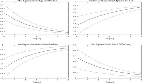
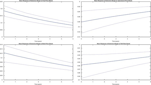
Figure 4. IRFs for extensive margins, full sample.

This figure displays mean impulse response functions of the extensive margin of exports to a one standard deviation shock in world prices. IRFs are calculated using all the countries in the sample.

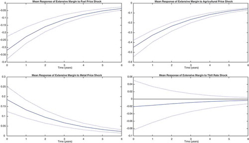
World price shocks have a significant impact on bilateral exports, both at the intensive and extensive margin. These effects are quite persistent and take more than 6 years before vanishing. An increase in agricultural prices determines an initial drop in the average export share of almost 16% (i.e., a drop of 0.006 units against a sample mean of 0.0367) and a fall in the average number of products exported of 5% (a fall of 0.042 from a mean of 0.8194). These responses capture the typical reaction to a (negative) supply shock, whereby the contraction in the world supply of agricultural goods leads to a spike in their price and a fall in world demand and exports. It is worth noticing that the contraction involves both the average volume of exports and their degree of diversification. An unexpected increase in metal prices also induces a fall in export size on average, in line with the narrative suggested above, though export diversification increases. The responses to fuel price shocks, on the contrary, appear to reflect (positive) demand shocks: the boost in world demand and in world prices is accommodated by larger and less diversified exports.⁷

Interest rate shocks affect exports mainly along the intensive margin (the response of the extensive margin is not significantly different from zero), and their effect is positive on average. In principle, a rise in the world real interest rate has ambiguous effects on a country’s exports. On the one side, world demand falls when interest rates are high because it is more costly to finance expenditure (the income effect), reducing a country’s exports. On the other side, world expenditure switches towards goods that are less expensive in a scenario of high interest rates (the substitution effect), for instance non-durable consumption goods as opposed to durable consumption and investment goods, or goods whose price has depreciated in real terms.

V. Sensitivity

Caution is needed in interpreting average responses, which may conflate ample heterogeneity across countries and over time. This section provides a thorough sensitivity analysis to consider the role of the exchange rate regime and the collapse of trade in 2008–2009.

Exchange rate regime

An important dimension of heterogeneity in our data set regards the exchange rate regime. Out of a total of 462 country pairs in the data set, 90 country pairs adopt fixed exchange rates between each other. In the baseline regression, we do not allow shocks to have different effects in fixed and flexible regimes. However, it is well known at least since Friedman (1953) that exchange rate flexibility may help cushion the effect of external shocks: in a situation where nominal prices are sluggish, exchange rate fluctuations allow a quicker adjustment in relative prices compared to fixed exchange rates. We should therefore observe larger price changes and smaller quantity movements in flexible regimes (the Friedman’s hypothesis). Ample evidence suggests the Friedman’s hypothesis holds indeed and flexible rates do help absorb external shocks (e.g., Broda 2004)⁸ Recent work based on dynamic, general equilibrium models with firms’entry suggests that the exchange rate regime, by affecting firms’ decision to enter foreign markets in the first place, may have persistent effects on the pattern of trade. (Bergin and Corsetti (forthcoming)) stress that flexible regimes may favour the production of differentiated goods and induce more export diversification compared to fixed regimes. The reason is that exchange rate flexibility helps stabilize markups, thereby favouring the creation of new products. Exchange rate variability also affects firms’ selection into export markets and reduces the volatility of entry over the business cycle (Cavallari and D’Addona 2018). A general insight from these studies is that exports fluctuations at the extensive margin may have non-negligible welfare consequences, adding a novel dimension to the traditional debate on the choice of the exchange rate regime. It is by now well understood that fixed exchange rates may be very costly whenever they constrain the variety of products that are exported and increase their variability over the business cycle (Hamano and Picard 2017).

To assess the role of exchange rates for the transmission of world shocks, we proceed in two steps.

First, we estimate the model separately for countries adopting fixed exchange rates (peggers) and for countries in flexible regimes (floaters) and provide a test of the difference between these two samples. In this way, we are able to detect eventual differences in the mechanism of propagation of shocks across regimes and test their statistical significance. Note that the vector of country-pair fixed effects in the baseline specification (5) reflects intra-European fixed effects in the sample of peggers.

Country pairs are classified using the IMF de facto classification (see Born et al., 2013), updated to match our sample period. For each year, a country pair is classified in the sample of ‘peggers’ if both countries have adopted a regime of ‘peg within horizontal bands’, or tighter, within the year. In all other cases, the country pair is classified in the sample of ‘floaters’.⁹ The list of ‘peggers’ and ‘floaters’ is reported in Appendix A.3. Notice that the sample of peggers comprises European countries and reflects intra-EMU trade. Figures 5 and 6 report the mean impulse responses of the intensive and the extensive margins of exports in the sample of, respectively, peggers and floaters.

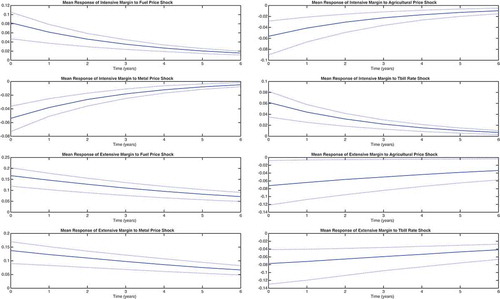
Figure 5. Peggers IRFs.

This figure displays mean impulse response functions of export margins to a one standard deviation shock in world prices. IRFs are calculated using countries classified as peggers. The first two rows display the responses of intensive margins while the last two rows display the responses of extensive margins.

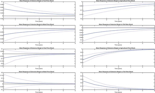
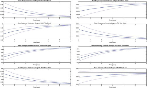
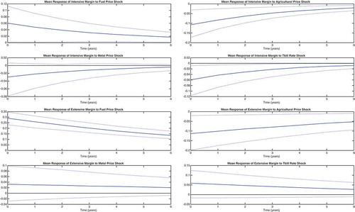
Figure 6. Floaters IRFs.

This figure displays mean impulse response functions of export margins to a one standard deviation shock in world prices. IRFs are calculated using countries classified as floaters. The first two rows display the responses of intensive margins while the last two rows display the responses of extensive margins.

The sign of almost all responses in the sub-samples remains unaffected compared to the full sample, confirming our interpretation about the nature of the shocks. Interest rate shocks provide a notable exception: in the sample of peggers, the response of the intensive margin becomes negative while that of the extensive margin turns significantly positive. The mechanism of adjustment appears to be different for floaters and peggers: while floaters mainly react at the intensive margin, by increasing the average volume of exports per product, peggers reduce export volumes and increase the range of products exported instead. This is consistent with ample evidence documenting the shock-absorbing properties of exchange rate flexibility. In the specific case of world interest rate shocks, countries that adopt flexible rates can depreciate their domestic currency to sustain their exports.

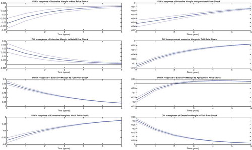
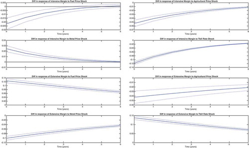
Notice that the responses of both margins are larger (in absolute value) in fixed regimes as far as shocks to interest rates and agricultural prices are concerned. The opposite is true for shocks to fuel and metals, which have only a negligible (statistically non-significant) effect in fixed regimes. To assess whether responses are systematically different across exchange rate regimes we follow Born et al. (2013) and compute a series of bootstrap-based indicators, one for each pair of shocks and margins, that represent the difference in the responses of peggers and floaters at the mean, the 95th percentile, and the 5th percentile of the distribution. These indicators, together with confidence bands at the 95% level, are shown in Figure 7. For shocks that imply a negative response in both regimes, like agricultural price shocks, a negative value of the indicator means a larger response under fixed rates. By the same token, a negative value of the indicator means a smaller response under fixed rates for shocks, like fuel price shocks, that have a positive impact in both regimes. For shocks that have opposed effects, like interest rate shocks, a value of the indicator different from zero is informative. All indicators are significant at the $95\mathrm{\%}$ level, and their value confirms the intuition given above: export margins in fixed regimes are more sensitive to interest rate and agricultural price shocks, while they are less sensitive to fuel and metal price shocks compared to flexible regimes. A higher variability at the intensive margin accords with the Friedman hypothesis that fixed rates should display more variation of average export volumes. High variability at the extensive margin, instead, is in line with the predictions of dynamic models of firms’ selection into export market.

Figure 7. IRFs differences between peggers and floaters.

This figure displays the difference, with $95\mathrm{\%}$ confidence interval, between peggers and floaters for mean impulse response functions. The first two rows display the results for intensive margins while the last two rows display the results for extensive margins.

Then, we consider a non-parametric specification of the baseline model (5) in which we allow for responses that vary non-monotonically with the exchange rate regime. For this purpose, we construct an indicator variable (dubbed ‘fix’) that takes a value of 1 when both countries are peggers and 0 otherwise, and interact the indicator with each shock in turn.¹⁰ In this way, we are able to gauge the economic and statistical significance of changes in the responses of peggers relative to the sample mean.

The coefficients on interacted terms measure the effect of shocks when countries adopt fixed exchange rates compared to the sample mean. They allow to quantify the extent to which the response of peggers deviates from the response of the average country-pair in the sample: a value of, say, 0.1 means that the response of peggers is higher by 0.1 units compared to sample average. This provides a measure of the impact of fixed rates that was not possible to identify with the sub-samples of peggers and floaters.

Table 2 reports the coefficients on shocks and interacted terms for the responses on impact (column entitled ‘impact’) and for the responses cumulated over 6 years (column entitled ‘cumulated’). A star indicates that the coefficient is significant at the 95% level.

Table 2. Controlling for the exchange rate regime.

	Intensive Margin
	Impact	Cumulated
Pa	−0.0630*	−0.2347*
Pf	0.0665	* 0.1972*
Pm	−0.0515*	−0.1567*
Tbill	0.0504*	0.1626*
Pa*Dfix	−0.0538	−0.1866
Pf*Dfix	−0.0138	−0.0345
Pm*Dfix	0.0139	0.0340
Tbill*Dfix	−0.1012*	−0.3181*
	Extensive Margin
	Impact	Cumulated
Pa	−0.4279*	−1.3602*
Pf	−0.3373*	−1.0547*
Pm	0.2019*	0.6346*
Tbill	−0.0626	−0.2142
Pa*Dfix	−0.2016	−0.6359
Pf*Dfix	0.1534	0.4810
Pm*Dfix	−0.1537	−0.4929
Tbill*Dfix	0.2193*	0.7026*

The responses to interest rate shocks appear significantly larger (in absolute value) when interacted with the indicator variable. Quantitatively, the effect is substantial: an increase in world interest rates determines a drop in the average export size of peggers on impact equal to 0.10 units (27%) against an average increase of 0.05 (16%). The effect on extensive margins is 0.22 (3%) for peggers against −0.06 (0.7%) on average. Moreover, these effects are persistent and significantly cumulate over a six-year horizon. As already noted, the opposite size of the responses reflects differences in the mechanism of adjustment. The results in Table 2 indicate a major role of exchange rates for interest rate shocks: exchange rate flexibility appears to help absorb the consequences of the shock. Pegging the exchange rate, on the contrary, appears to improve the capacity to adjust at the extensive margin. As regards price commodity shocks, we observe significant differences neither in the mechanism of adjustment nor in the magnitude of the impact.

Overall, our findings support the view that exchange rate flexibility matters for the transmission of shocks at both the intensive and extensive margin. In departing from studies that use single measures of world prices, we show that the ability of flexible rates to cushion the effects of world price shocks depends on the shock considered. Flexibility appears to be important for shocks, like interest rates in our data, that imply large substitution effects.

The great trade collapse

In this section, we investigate the role of the ‘great trade collapse’ for the dynamics of the model. The collapse occurred between the third quarter of 2008 and the second quarter of 2009. It was severe – the steepest fall of world trade in recorded history and the deepest fall since the Great Depression – and synchronized. The rebound was equally impressive, characterized by outsized fluctuations in trade volumes.¹¹ Many studies observe that, despite trade, volumes have recovered relatively quickly to the pre-crisis levels, their volatility does not appear to be mean-reverting.¹² The great trade collapse may therefore constitute a structural break in the propagation of shocks.

To shed some light on the question, we consider a non-parametric specification in which responses vary non-monotonically before and after the great trade collapse. An indicator variable (dubbed ‘period’) that assumes a value of 1 for the years 2008 to 2018 and a value equal to 0 otherwise is interacted with the responses of each shock. The coefficients on interacted terms capture the effect of shocks in the post-crisis period compared to the whole period. So a value of, say, 0.1 reflects a response that is higher by 0.1 units in the post-crisis period with respect to the sample mean. Table 3 reports the coefficients on shocks and interacted terms for the responses on impact (column entitled ‘impact’) and for the responses cumulated over 6 years (column entitled ‘cumulated’). A star indicates that the coefficient is significant at the 95% level.

Table 3. Controlling for the great trade collapse.

	Intensive Margin
	Impact	Cumulated
Pa	−0.1184*	−0.3943*
Pf	−0.0728*	−0.2287*
Pm	−0.0566*	−0.1601*
Tbill	0.0032	0.0061
Pa*Dperiod	0.0761*	0.1778
Pf*Dperiod	0.3788*	1.1721*
Pm*Dperiod	−0.0903*	−0.3177*
Tbill*Dperiod	0.1527*	0.4590*
	Extensive Margin
	Impact	Cumulated
Pa	−0.0541	−0.2159
Pf	0.1322*	0.4057*
Pm	0.3445*	1.0636*
Tbill	−0.0488	−0.1706
Pa*Dperiod	−0.9959*	−3.0717*
Pf*Dperiod	−0.8536*	−2.6062*
Pm*Dperiod	−0.3462*	−1.1019*
Tbill*Dperiod	−0.5181*	−1.5894*

The responses of both margins to almost all shocks are larger (in absolute value) after the great trade collapse. These effects are considerable. We document an increase in the post-crisis responses of intensive margin on impact that is equal to 20%, 80%, and 25% for, respectively, fuel price, metal price and interest rate shocks. The increase is of a comparable size for extensive margins, and in the cases of fuel and metal prices, it implies a change also in the direction of the effect. Notice that most of these effects are persistent.

Caution is needed in interpreting these findings. A limit of our experiment is that we cannot say whether large post-crisis responses reflect higher volatility of world shocks or higher sensitivity to external conditions, or any combination of the two. Identifying the factors that explain these dynamics is an interesting challenge for future research.

VI. Conclusions

This paper has provided evidence that world price shocks play a remarkable role for aggregate exports, affecting both average export volumes and export diversification. The analysis builds on a panel VAR model with exogenous factors, where the endogenous bloc comprises export margins measured on a country-pair basis, and computed with data at the four-digit SITC. The exogenous bloc includes world commodity prices, namely agricultural, metal and fuel prices, together with world real interest rates. We find that all shocks have a significant impact on at least one margin and most of them on both margins. We document substantial heterogeneity in the responses depending on the shock considered, the exchange rate regime and the great trade collapse. Despite heterogeneity, one conclusion emerges with clarity: swings in world prices are important and their importance has increased after the great trade collapse.

The evidence in the paper has relevant policy implications. The large and persistent effects we have documented suggest that policies aimed at promoting trade should become more aggressive in periods of high volatility of world prices. Moreover, they should consider that adjustment may occur mainly at the intensive or at extensive margin depending on exchange rate flexibility. Our findings are a first step towards understanding the mechanism of propagation of disaggregated world shocks. Further evidence is needed to evaluate more disaggregated measures, and extend the analysis to developing countries that are particularly vulnerable to world shocks.

Disclosure statement

No potential conflict of interest was reported by the authors.

Notes

¹ Ghironi and Mélitz (2005) is among the pioneering studies in this literature. Ghironi (2018) provides a comprehensive analysis of the state of the art.

² The countries are: Australia, Belgium, Canada, Czech Republic, Finland, France, Germany, Iceland, Italy, Japan, Korea, Luxembourg, Netherlands, Portugal, Spain, Sweden, Mexico, New Zealand, Norway, Switzerland, United States and United Kingdom.

³ WITS, see http://wits.worldbank.org/wits/.

⁴ See https://unstats.un.org/unsd/trade/sitcrev4.htm.

⁵ Changing the order of variables in (4) is immaterial for our analysis. Results under alternative identification are available upon request.

⁶ Impulse response functions and confidence intervals are obtained by Monte Carlo simulations with 1000 replications.

⁷ Our sample includes world leaders in coal, gas and oil markets. Australia, the United States and Canada are leading exporters of coal, Norway, Australia, the United States, Germany and Canada are among the 10 largest exporters of gas, and Canada is the fourth exporter of oil in the world.

⁸ (Hoffman 2007) provide support to the Friedman’s hypothesis for a sample of 42 developing countries and (Ghosh, Ostry, and Qureshi 2015) for 182 countries.

⁹ More nuanced classifications of exchange regimes are hard to implement in our panel, because of the small number of country pairs adopting intermediate regimes. See Cavallari and D’Addona (2017) for a thorough discussion.

¹⁰ The vector of world shocks includes four additional terms capturing the interaction of each shock with the indicator variable. We also include interaction terms in the vector of country-pair fixed effects to capture fixed effects that are specific for peggers.

¹¹ According to the World Trade Organization, the volume of trade recovered to its pre-collapse level by the first quarter of 2011 (see Huo-can and Yi-qing, 2011).

¹² For a survey of the literature examining the causes and consequences of the “great trade collapse” see Bems, Johnson, and Kei-Mu (2013).

Appendix

A.1. Robustness

In this section, we replicate our empirical analysis using the simple measure (see Eaton and Fieler 2019). This is meant to address concerns about the role of changes in export value for the identification of the set of products a country exports. Clearly, the same concerns do not extend to intensive margins, which are defined as export value per product. The exercise provides a robustness check for our findings.

As in the main text, we start with an overview of the data, in Figure 1A and Table A1.

Figure A1. Distribution of extensive margins.

This table displays the median, the ${25}^{th}$ and the ${75}^{th}$ percentile of extensive margins, calculated as Eaton and Fieler (2019), for all the countries in the sample.

Table A1. Summary statistics with extensive margins calculated as Eaton and Fieler (2019).

	σxm	σim	σxm/σim	ρ(xm, ∆gpdh)	ρ(xm, ∆gpdf)	ρ(im, ∆gpdh)	ρ(im, ∆gpdf)
Australia	0.258	0.065	3.967	0.016	0.000	−0.008	0.085
Belgium	0.098	0.068	1.439	−0.095	−0.238	0.007	0.025
Canada	0.182	0.042	4.334	−0.113	−0.123	−0.059	0.058
Switzerland	0.111	0.028	3.982	0.040	−0.181	0.109	−0.034
Czech Republic	0.206	0.009	23.397	0.028	−0.297	−0.020	−0.195
Germany	0.038	0.143	0.268	−0.059	−0.180	0.234	−0.036
Spain	0.126	0.064	1.956	−0.083	−0.199	0.027	−0.092
Finland	0.169	0.021	7.865	−0.023	−0.194	0.031	−0.033
France	0.076	0.046	1.640	−0.012	−0.168	0.104	−0.052
United Kingdom	0.052	0.042	1.244	0.033	−0.147	0.150	0.048
Iceland	0.129	0.018	6.972	0.114	−0.165	−0.091	0.110
Italy	0.066	0.030	2.221	−0.041	−0.200	0.126	−0.062
Japan	0.179	0.101	1.779	0.053	0.044	0.383	0.285
Korea Rep.	0.194	0.030	6.519	−0.136	−0.098	0.187	0.103
Luxembourg	0.243	0.002	141.370	−0.052	−0.227	0.075	−0.020
Mexico	0.258	0.029	8.949	−0.028	−0.154	0.004	0.012
Netherlands	0.086	0.034	2.529	−0.091	−0.209	−0.066	−0.186
Norway	0.200	0.022	9.093	−0.030	−0.117	0.001	−0.022
New Zealand	0.250	0.013	19.857	0.002	−0.043	−0.092	0.120
Portugal	0.217	0.016	13.188	−0.170	−0.227	0.216	−0.078
Sweden	0.116	0.050	2.300	0.003	−0.193	−0.025	−0.007
United States	0.098	0.182	0.541	0.004	−0.051	0.040	0.077
Mean	0.152	0.048	12.064	−0.029	−0.153	0.061	0.005
Standard deviation	0.070	0.044	29.516	0.067	0.082	0.119	0.106

Extensive margins measured by the fraction of products behave similarly to the HK measure: the distribution is skewed towards high values, indicating substantial export diversification, and large countries appear to diversify more than small countries. Moreover, extensive margins are more volatile than intensive margins (the ratio of standard deviation is 12:1) and are weakly correlated with output in the origin and destination country. Not surprisingly, the correlation between the simple and the HK measure is high. The similar behaviour of the two measures might reflect a limited role for products that are of scarce importance in world trade in our data set.

Then, we provide impulse responses for the full sample and for the sub-samples of floaters and peggers in Figures A2, A3, and A4, respectively.

Figure A2. Full sample IRFs.

This figure displays mean impulse response functions of the extensive margins, calculated as Eaton and Fieler (2019), to a one standard deviation shock in world prices.

Figure A3. Floaters IRFs.

This figure displays mean impulse response functions of the margin of exports to a one standard deviation shock in world prices. IRFs are calculated using countries classified as floaters. The first two rows display the responses of intensive margins while the last two rows display the responses of extensive margins calculated as Eaton and Fieler (2019).

Figure A4. Peggers IRFs.

This figure displays mean impulse response functions of the margin of exports to a one standard deviation shock in world prices. IRFs are calculated using countries classified as peggers. The first two rows display the responses of intensive margins while the last two rows display the responses of extensive margins calculated as Eaton and Fieler (2019)

Using the simple measure is immaterial for our results: the responses are very similar to those obtained in the main text. The same is true for the subsequent steps in the analysis. The responses are significantly different across exchange rate regimes (see Figure A5).

Figure A5. IRFs differences between peggers and floaters.

This figure displays the difference, with $95\mathrm{\%}$ confidence interval, between peggers and floaters for mean impulse response functions. The first two rows display the results for intensive margins while the last two rows display the results for extensive margins calculated as Eaton and Fieler (2019).

A.2 Data

Table A2. Data sources and transformations.

Original series	Source	Data transformation
Nominal GDP	OECD.StatExtracts	log differenced, deflated using the GDP Deflator
GDP Deflator	OECD.StatExtracts	None
US Treasury Bill Rate	FRED II	deflated using the US CPI
Bilateral export flows per product	UN Comtrade database	decomposition into extensive and intensive margins
Commodity price indices	World Bank Commodity Price Data

A.3 Peggers and floaters

Table A3. List of countries and their classification.

Peggers	Floaters
Belgium	Australia
Finland	Canada
France	Czech Republic
Germany	Iceland (After 2001)
Iceland (Before 2001)	Japan
Italy	Mexico
Luxembourg	New Zealand
Netherlands	Norway
Portugal	South Korea
Spain	Sweden
	Switzerland
	United Kingdom
	United States

References

- Bems, R., R. Johnson, and Y. Kei-Mu. 2013. “The Great Trade Collapse.” Annual Review of Economics 5 (1): 375–400.
- Bergin, P. R., and G. Corsetti. forthcoming. “Beyond Competitive Devaluations: The Monetary Dimensions of Comparative Advantage.” American Economic Journal: Macroeconomics.
- Born, B., F. Juessen, and G. J. Muller. 2013. “Exchange Rate Regimes and Fiscal Multipliers.” Journal of Economic Dynamics and Control 37 (2): 446–465.
- Broda, C. 2004. “Terms of Trade and Exchange Rate Regimes in Developing Countries.” Journal of International Economics 63 (1): 31–58.
- Cavallari, L. 2013. “Firms’ Entry, Monetary Policy and the International Business Cycle.” Journal of International Economics 91: 263–274.
- Cavallari, L., and S. D’Addona. 2015. “Exchange Rates as Shock Absorbers: The Role of Export Margins.” Research in Economics 69 (4): 582–602.
- Cavallari, L., and S. D’Addona. 2017. “Output Stabilization in Fixed and Floating Regimes: Does Trade of New Products Matter?” Economic Modelling 64: 365–383.
- Cavallari, L., and S. D’Addona, “External Shocks, Trade Margins and Macroeconomic Dynamics,” Mimeo, Universitá Roma Tre 2018.
- Eaton, J., and A. C. Fieler, “The Margins of Trade,” NBER Working Papers 26124, National Bureau of Economic Research 2019.
- Everaert, G., and L. Pozzi. 2007. “Bootstrap-based Bias Correction for Dynamic Panels.” Journal of Economic Dynamics and Control 31 (4): 1160–1184.
- Fernández, A., S. Schmitt-Grohé, and M. Uribe. 2017. “World Shocks, World Prices, and Business Cycles: An Empirical Investigation.” Journal of International Economics 108: S2– S14.
- Fomby, T., Y. Ikeda, and N. V. Loayza. 2013. “The Growth Aftermath of Natural Disasters.” Journal of Applied Econometrics 28 (3): 412–434.
- Friedman, M. 1953. “The Case for Flexible Exchange Rates.” In Essays in Positive Economics, edited by University of Chicago Press, Chicago, IL: University of Chicago Press, 159–205.
- Ghironi, F. 2018. “Macro Needs Micro.” Oxford Review of Economic Policy 34 (1–2): 195–218.
- Ghironi, F., and M. J. Mélitz. 2005. “International Trade and Macroeconomic Dynamics with Heterogeneous Firms.” The Quarterly Journal of Economics 120 (3): 865–915.
- Ghosh, A. R., J. D. Ostry, and M. S. Qureshi. 2015. “Exchange Rate Management and Crisis Susceptibility: A Reassessment.” IMF Economic Review 63 (1, May): 238–276.
- Hamano, M., and P. M. Picard. 2017. “Extensive and Intensive Margins and Exchange Rate Regimes.” Canadian Journal of Economics/Revue Canadienne D’ã©conomique 50 (3): 804–837.
- Hoffman, M. 2007. “Fixed versus Flexible Exchange Rates: Evidence from Developing Countries.” Economica 74 (295): 425–449.
- Hummels, D., and P. J. Klenow. 2005. “The Variety and Quality of a Nation’s Exports.” American Economic Review 95 (3): 704–723.
- Huo-can, W., and W. Yi-qing. 2011. “Trade Growth to Ease in 2011 but despite 2010 Record Surge, Crisis Hangover PersistsWorld Trade 2010, Prospects for 2011.” World Trade Organization Focus, no. 3: 13.
- Kose, A. 2002. “Explaining Business Cycles in Small Open Economies: ‘how Much Do World Prices Matter?’.” Journal of International Economics 56 (2): 299–327.
- Mendoza, E. 1995. “The Terms of Trade, the Real Exchange Rate, and Economic Fluctuations.” International Economic Review 36 (1): 101–137.
- Naknoi, K. 2015. “Exchange Rate Volatility and Fluctuations in the Extensive Margin of Trade.” Journal of Economic Dynamics and Control 52: 322–339.
- Nickell, S. J. 1981. “Biases in Dynamic Models with Fixed Effects.” Econometrica 49 (6, November): 1417–1426.
- Pesaran, M. H., and Z. Zhao. 1999. “Bias Reduction in Estimating Long-run Relationships from Dynamic Heterogeneous Panels.” In Analysis of Panels and Limited Dependent Variable Models, edited by C. Hsiao, M. H. Pesaran, K. Lahiri, and L. F. Lee, 297–322. Cambridge, UK: Cambridge University Press.
- Schmitt-Grohé, S., and M. Uribe. 2018. “How Important are Terms-of-trade Shocks?” International Economic Review 59 (1): 85–111.