The influences of covid-19 pandemic on macroeconomic indexes for European countries

ABSTRACT

The Covid-19 pandemic had a major impact in the entire world, both sanitary and economic. The purpose of this study is to analyse the European countries from this point of view. The main economic indicators related to import, wages, labour productivity, consumption, taxes, gross domestic product (GDP), as well as variables related to Covid-19 pandemic measures were considered in order to estimate the impact that pandemic measures have in economy. Principal component analysis was performed in order to reduce the dataset dimensionality and to create new indicators. Selected European countries are characterized and compared using principal components analysis outputs while regression is used to identify an influence of independent variables on GDP. The main results show that, comparing European countries economic situation in 2020 with the previous 2 years and considering variables that show the adopted closure measures, the Covid-19 pandemic have influenced the GDP from European countries.

KEYWORDS:

• Covid-19
• macroeconomic
• principal components
• regression
• dummy variables

I. Introduction and literature review

The impact that Covid-19 pandemic has on economy is a widely discussed issue since the beginning of 2020. The increasing number of cases led to urgent measures like lockdown. In Europe, since February–March 2020, most countries had an ascending trend for the number of cases; many of them declared state of emergency and had general lockdown. The social distancing required measures forced all activity sectors to reconsider their activity, for example: home delivery for restaurants, online shopping for retailers, working from home for companies, online learning and others. Each decision/measure had an impact in the economic output. The regression models in this paper show this impact. Measures taken by countries affected by the pandemic to reduce the spread of the virus have an economic cost (Abiad, et.al., 2020). Considering the entire Europe as a system composed of the economy of each individual country, it is possible to say that a small change in the system, such as the state of emergency for a country, could cause a major imbalance to the big system. For the economic system these measures have two important effects: a short-term effect or an immediate impact and a long-term effect, not immediately visible. Although most of the countries that had a lockdown situation in March–April 2020 came with economic recovery measures, the impact for economic system remains significant (Fernandes, 2020).

The main hypotheses to test in this research is that the measures to reduce the spread of the Covid-19 virus have caused instability of the European countries’ economies. The short-term effect is analysed, by considering quarterly variables for 2020 (Q1 and Q2), but cross-sectional datasets, not time series. Among the many forms of economic instability, the most significant are as follows: cyclical fluctuations in GDP, investment, consumption, employment, unemployment, inflation and others. The objective of economic policy is to seek to stabilize the functioning and development of the economy, thus providing viable solutions for social and political stability (Atkeson, 2020). On the other hand, the economy can also be considered as a complex adaptive system and characteristics like coevolution, connectivity and interdependence (Mitleton-Kelly 2003) are the most relevant in demonstrating that a small change in a connected system, for example, like health, can lead to big changes in other systems, the economy. These measures have influenced the relationships between indicators, which are well-known and verified before the pandemic.

Recent studies show a high interest of researchers for the impact of pandemic in different areas of interest, like social, poverty, consumption, economic. Martin et al. (2020) analysed the impact of pandemic on household consumption and poverty, taking into account the two identified periods: the crisis period and the recovery period. Using modelling, the authors concluded that in the absence of social protection, the impact of pandemic ‘lead to a massive economic shock to the system’ (Martin et al. 2020). Another study (McKibbin 2020b) starts from the economic situation in China and provides seven scenarios to model the evolution of Covid-19 pandemic in 2020 and its impact in the economy. Authors (McKibbin, et.al., 2020a and 2020b) suggested that a series of policies and economic measures are required on short-term and on long-term.

Another study analyzes the impact of Covid-19 on the United Kingdom economy (Keogh-Brown et al. 2020), using multi-sectorial models, like CGE, and computing the impact for multiple scenarios. The main conclusions of this research are that the economic impact can measure in terms of the duration of mitigation or suppression policies (Keogh-Brown et al. 2020). In the same year, Mariolis, Rodousakis, and Soklis (2020) use a multi-sectorial model to study the COVID-19 multiplier effects of tourism on macroeconomic indicators like: gross domestic product (GDP), total employment, and trade balance of the Greek economy. Their results show that tourism in Greece, directly affected by pandemic-related measures, has a significantly impact on the studied indicators. On the other hand, for Germany, Gandjour (2020) analyse the life-tables model and several scenarios ‘to estimate the impact of a shutdown on lives saved and life years gained’ (Gandjour 2020) and correlates the results with GDP. Another research regarding the first Covid-19 pandemic wave reveals that, in European countries, the spread of the virus is not the only factor that have economic impact, but: ‘the results suggest that a region’s trade relations represent an important indirect channel through which Covid-19 related disruptions affect regional economic activity’ (Meinen, Serafini, and Papagalli 2021).

Looking outside Europe (to the countries from other continents), like United States of America, Makridis and Hartley (2020) estimate a five percent decline in real GDP growth for every one month of partial economic lockdown, using several assumptions. The real impact of Covid-19 pandemic in U.S. GDP was −31.2% in 2020Q2% change from preceding quarter), according to a report of the Congressional Research Service from November 2021.¹ For Africa (Jayaram et al. 2020), the GDP growth is estimated to decrease with about three percent to eight percent in 2020, although the pandemic did not strike as fast as in Europe. On reason for this situation is that the rate of covid-19 transmission in Africa appears to be slower than in Europe, in March 2020 (Jayaram et al. 2020). In Indonesia, in a recent study (Putra and Arini 2020), the prediction of GDP for Indonesia (regional, then national) is made taking into consideration the mobility of people from 34 provinces. Authors uses cluster analysis to group the provinces into 5 groups and regression to estimate the GDP growth for 2020Q1 and 2020Q2, their findings being similar to real computed values for GDP growth. In China, one study (Chen, Qian, and Wen 2020) shows that the pandemic restrictions had a major impact in the consumption analyzed in 214 cities: ‘all 214 cities experienced significant consumption decreases, with magnitudes ranging from 14% to 69%’ (Chen, Qian, and Wen 2020). Another research for China economy reveals that ‘the Covid-19 pandemic has had a considerable negative effect on China’s GDP growth’ (Gunay, Can, and Ocak 2021), mostly for the first quarter of 2020. In Indonesia, a recent study (Solihin et al. 2021) studies (using econometric models), the economic growth at regional level and conclude that ‘the government also needs to improve public spending efficiency by applying better governance and accountability’ (Solihin et al. 2021). Another study about Indonesia (Pasaribu et al. 2021) consider spatial simultaneous model to study that pandemic vulnerability in Indonesian regions and show that ‘COVID-19 pandemic vulnerability levels have socio-economic spillover effects on neighboring areas in Indonesia’ (Pasaribu et al. 2021). Econometric models are also used in another research (Chen et al. 2020) that take into consideration many countries that implemented lockdown or closure measures and that are affected by Covid-19 pandemic. Among the results obtained in this research: ‘countries implementing workplace and school closures experienced larger contractions in GDP growth in the first half of 2020, while countries implementing other measures do not show significant contractions in economic growth’ (Chen et al. 2020). A comparison between Europe and United States regarding the impact of Covid-19 pandemic shows that ‘regions and countries where the outbreak is more sizeable experience significantly more severe economic losses’ (Chen et al. 2020). Another econometric research analysis (for more than 150 countries) that studies the globalization and Covid-19 pandemic, shows that the virus spread and the number of deaths is positively associated with the level of globalization (Farzanegan, Mehdi, and Hassan 2021). Studying the effects of Covid-19 pandemic as global recession, the ‘medium-term output losses are anticipated to be lower than after the global financial crisis’, especially for ‘emerging market and developing economies’ (Barrett et al. 2021). The analysis of 44 countries shows that countries that responded strongly with ‘a COVID-19 elimination strategy’ are less affected (from macroeconomic point of view – GDP growth) than countries “which aim to ‘live with the virus’ and hence respond slowly and in a gradual way to rising infections” (Konig, Winkler, and Xue 2021). By analyzing over 40 countries, another study presents the results that the impact of pandemic “on countries’ economies was evaluated, showing an average negative result of 3% in the GDP for every 1000 people per million inhabitants” (de la Fuente-Mella et al. 2021).

Other relevant research papers regarding the impact of Covid-19 pandemic in economy are related to stock market, a market that is, in general, very impacted even by small changes in economy. Studies show that ‘all stock markets (for seven countries: Canada, China, France, Germany, South Korea, the UK and the US) responded to COVID-19 shocks mostly negatively’ (Tchatoka, Julia Puellbeck, and Masson 2022). In US: ‘stock market volatility is positively affected by the death rate (bad news) while the recovered rate (good news) has a negative impact on the US stock market volatility’ (Baek and Lee 2021), while in China: ‘investors are more risk appetite for the stocks that included in the coronavirus and influenza indices after the outbreak of COVID-19 pandemic, compared to other financial indices’ (Corbet et al. 2021).

This paper presents in the first part several studies that are relevant for the research. The second section is reserved to the presentation of the datasets, data sources, methodologies and the main methods and techniques used to finalize the study. The third section presents the main results and discussions, while the last section shows the conclusions and the further research ideas.

II. Datasets and methodologies

The main dataset is composed by the indicators, presented in Table 1 from below, that show the consumption of households and general government, the import, the wages and the salaries, the subsidies or the taxes on production and imports. These macroeconomic indicators were selected in order to test their influence on GDP growth, taking into consideration their modification during pandemic (for example, the real labor productivity per person could decrease as a consequence of working from home and may lead to a decrease of performance and production that could have an impact in GDP growth – these hypotheses are to be tested in the regression models). The GDP (in percentage change on previous period) is also considered as dependent variable, as well as several dummy variables that indicate the measures adopted in the first 6 months of 2020 regarding the Covid-19 pandemic, and the impact (quantified in the number of cases) of pandemic in the first semester from 2020.

Table 1. The variables used for models

indicator code	indicator name
I8	Final consumption expenditure of general government
I14	Imports of goods and services
I19	Employers’ social contributions
I20	Subsidies
I21	Taxes on production and imports less subsidies
I26	Real labour productivity per person
I36	Wages and salaries Agriculture, forestry and fishing
I37	Wages and salaries Industry (except construction)
I44	Final consumption expenditure of households
I55	Government consolidated gross debt
School	Requiring school closing (all levels or only some levels)
Workplace	Require closing (or work from home) for all or for some categories
Stay_home	Require not leaving house
Internal	Internal movement restrictions
Ban_arrivals	Ban arrivals from some regions or all regions or total border closure
Cases	1 if number of cases in 2020Q1 is above 2000, and 1 if number of cases in 2020Q2 is above 10,000

Eurostat is the main data source for the macroeconomic indicators (GDP and indicators with code from I8 to I55), the European Center for Disease Prevention and Control is the data source for the number of Covid-19 cases, while the Oxford COVID-19 database represents the main source for dummy variables (coded with school, workplace, stay_home, internal or ban_arrivals). All macroeconomic indicators from Table 1 from below are computed as percentage of GDP or percentage change on previous period (I26).

The dummy variables that represent the main restrictions are computed for 2020Q1 and 2020Q2. The value of each dummy variable is 1 if the number of days (or cases for the last variable) is above each value presented in Table 2 from below. Each value from below represents in average (for selected countries), the number of days in each quarter when the restriction (closure policy) was adopted. For example, the school was required to be closed for all levels (or only some levels) for 20 days in average in Q1–2020, from all 91 days, while in Q2–2020, for 79 days in average. If, in a specific country, the number of days exceeded 20 for Q1–2020 and 79 for Q2–2020, then the value for ‘school’ dummy variable is 1, else is 0. For the number of cases, the values 2000 and 10,000 are close to median value for each quarter (the media values are as follows: 2055 for Q1–2020, and 8048 for Q2–2020).

Table 2. The dummy variable criteria

Variable	2020Q1	2020Q2
School	20	79
Workplace	15	67
Stay_home	8	32
Internal	7	32
Ban_arrivals	24	79
Cases	2000	10,000

The observations were considered as the majority of European countries, but, after the significantly too high or too low values for each indicator were eliminated, 23 countries, including Romania, were selected. Six datasets are considered in order to compare the results: the first two-quarters, Q1 - January to March and Q2 - April to June, for 2018, 2019 and 2020. Therefore, the final database consists of six individual cross-sectional data sets (for 2018 Q1, 2018 Q2, 2019 Q1, 2019 Q2, 2020 Q1 and 2020 Q2), with 23 European countries each set. The data sets for 2018 and 2019 have only the macroeconomic indicators described in Table 1, while the data sets for 2020 contain, in addition, several variables regarding the Covid-19 pandemic situation (describing the impact of the number of cases, or the main closure policies adopted by countries).

Regarding the methodological approach, we use data analysis methods, in order to reduce the number of variables and to create new uncorrelated indicators. Principal component analysis (PCA) is the most widely used method, and it is based on the analysis of the correlation matrix. In this way the new indicators are computed. The main feature of these calculated indicators is: they are uncorrelated, while the original variables that are strongly correlated. The purpose of using PCA in this study is to eliminate the correlations between variables, by creating new variables named principal components. Each principal component is a linear combination of all original variables, with the eigenvectors of correlation matrix as weights. The values of weights, as well as the correlations between the original variables and principal components show that each new combination has a signification.

On the other side, the principal component regression (PCR) aims are the estimation a regression model using principal components like regressors. But not all the principal components that are computed are used in the regression model. Only the first k components are kept further in the analyses that consider several aspects: cover a significant percentage of total information from the original variables (over 70%–80%) or have the variance higher than 1, according to the Kaiser criteria. The main advantage of using PC (principal components) as independent variables for the regression model is that the multicollinearity hypothesis of the model is fulfiled by default. In the same time, the main disadvantage represents the idea that the eliminated PC might contain pieces of information from variables that explain the variance of the dependent variable, so that the principal components that have low variances may have some importance, in some cases this importance is a significance one. Each principal component is computed as maximizing the information left uncovered by the previously component, so that there is no common information in two different principal components, which leads to zero correlations. In order to identify if the eliminated principal components have a significant contribution to the regression models, a comparison is made between several models.

III. Results and discussions

Descriptive statistics and principal components analysis

For the first analysis of the data sets it is necessary to study the correlation matrix between the original variables. Thus, a negative correlation coefficient shows that an increase of one variable leads to a decrease of the other variable, while a positive correlation coefficient shows a change in the same direction for both variables.

Figure 1. Correlation matrix for datasets 2019-Q2 (left) and 2020-Q2 (right).

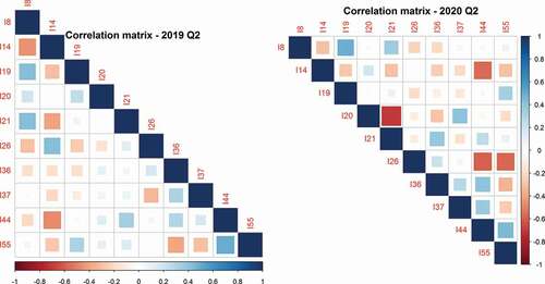
The correlation matrix in Figure 1, for both Q2 2019 and Q2 2020 shows that the variables are correlated. This can indicate a problem in a regression model, because of multicollinearity. The principal component analysis technique was applied on each dataset, in order to compute new indicators. These new indicators are fewer than the original variables, but advantage is that they have a significant amount of information and are uncorrelated.

In Table 3, the main results of principal components analysis are presented: the number of original variables; the number of principal components relevant for the analysis; the percentage of information (from 100%) considered in the selected principal components and the percentage of lost information. The number of principal components (PC) is determined taking into consideration several criteria like: Kaiser, percentage of information and scree plot. The Kaiser criteria states that the number of PC which must be kept further in the analysis is the number of PC with the level of variance above 1, while the coverage percentage criteria says that the number of PC considered should take into account the total percentage of information of about 70–80%. Therefore, the number of selected components is five for all considered datasets.

Figure 2. Correlation matrix – original variables and PC.

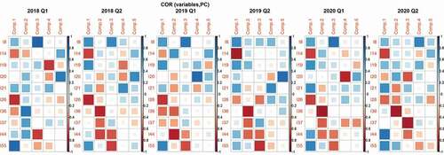
Table 3. The main results of the principal component analysis

Dataset	Number of variables	Number of PC	% of information	% of loss
2018Q1	10	5	80.33%	19.67%
2018Q2	10	5	81.30%	18.70%
2019Q1	10	5	79.25%	20.75%
2019Q2	10	5	82.63%	17.37%
2020Q1	10	5	82.64%	17.36%
2020Q2	10	5	87.36%	12.64%

5 PCs consider over 80% of total information (79.25% for 2019-Q1), as the lost information is 100%-% of information.

Figure 2 describes the correlation matrices of the original variables with PC for all six datasets (from left to right: from 2018 Q1 to 2020 Q2). The number of each PC is presented in the upper part of each figure (as Comp.1, Comp.2, to Comp.5), while the code of each original variable is presented in the left part of each figure. The scale is presented in the right part of each figure: the red colour shows a negative correlation coefficient between a variable and a principal component, while shades of blue show a positive correlation coefficient. It is interesting to notice that the pattern of PC is almost the same in time, with slightly changes for 2020 Q2 (when the pandemic restrictions started to have effects on the main macroeconomic indicators). Taking into consideration these correlations, as well as the contribution of each variable to the variance of each PC, it is possible to give a meaning for each PC. For 2018 datasets, one PC is very correlated with subsidies variable, another with consumption expenditures (households and general government), another with trade, real labour productivity and government debt, the main public income (represented by employers’ social contributions and taxes on production and imports) is another principal component, while wages and salaries (for agriculture and industry) represent the fifth component. The correlations between principal components and original variables slightly differ for 2019 datasets, comparing with 2018, while in 2020, the difference is obvious: for example, the subsidies and wages and salaries for industry are highly correlated with the same principal component.

Figure 3. First PC score and GDP −2018 Q1 vs. 2019 Q1.

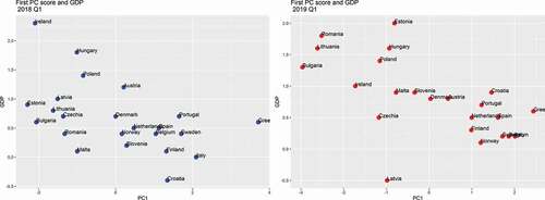
In Figure 3 it can be observed the representation of GDP_gr variable and the first principal component from 2018Q1 and 2019Q1 datasets. The first principal component has the highest variance and contains the most information from the original variables: 24% for 2018Q1 dataset and 24.83% for 2019Q1. In both situations, it is noticeable that, countries with high values for the first principal component have lower GDP_gr than other countries, taking into consideration that PC1 is negatively correlated with real labor productivity per person and positively correlated with government consolidated gross debt.

Figure 4. The number of adopted closure policies −2020 Q1 vs. Q2.

Output obtained in R software; Starting February-March 2020, the number of cases increased rapidly in most European countries, so one closure measure was not enough anymore.

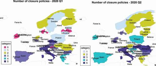
Figure 4 from above shows a synthesis of the number of adopted closure measures for covid-19 pandemic in 2020 (Q1 vs. Q2). The sum of dummy variables for each country represents the number of measures that were adopted more (than average) in each quarter. These measures are highly correlated with the number of cases and the incidence of the covid-19 pandemic. For example, in the first three months from 2020, the virus spread very fast in Italy, Spain, Belgium or Austria and less in Latvia, Estonia, Lithuania or Slovenia, and these countries adopted very fast many restrictive measures in order to limit the spread of the virus. In the next 3 months (Q2–2020), more European countries were affected by the pandemic, and the closure measures were adopted one by one in each country, reaching to lockdowns.

Regression results

In order to identify the impact of pandemic on GDP, multiple-regression models were analysed, all having GDP_gr as dependent variable. Each dataset was considered independently (cross-sectional data), at the same moment of time, as the seasonal effect was not taken into account. Each model is computed for original variables, all principal components and selected principal components.

Figure 5. Regression models results for 2018 and 2019 - Q1 and Q2.

Output obtained in R software²; t statistics is in parantheses,***, **, * refers to level of significance: 1%, 5%, 10%

Figure 5 from above show the regression main results for 2018 and 2019 datasets. Each dataset represents a quarter: Q1 or Q2. A comparison between original variables (first figure from the left) and principal components (next two figures from the right) confirm that, taking into account several principal components (5 PCs with about 80% of information), the R² is lower than considering all principal components (or initial variables). Confirming this hypothesis, initial variables were considered for further analyses, all models having an associated p-value for F-statistic that is below 0.05, validating the models. The estimated models are

(1) $\begin{array}{rl}& GDP\mathrm{\_}g{r}^{\left(Q_i\right)}={\beta }_0^{\left(Q_i\right)}+{\beta }_1^{\left(Q_i\right)}{I}_8^{\left(Q_i\right)}+{\beta }_2^{\left(Q_i\right)}{I}_{14}^{\left(Q_i\right)}\\ & +{\beta }_3^{\left(Q_i\right)}{I}_{19}^{\left(Q_i\right)}+{\beta }_2^{\left(Q_i\right)}{I}_{20}^{\left(Q_i\right)}+{\beta }_5^{\left(Q_i\right)}{I}_{21}^{\left(Q_i\right)}+{\beta }_6^{\left(Q_i\right)}{I}_{26}^{\left(Q_i\right)}\\ & +{\beta }_7^{\left(Q_i\right)}{I}_{36}^{\left(Q_i\right)}+{\beta }_8^{\left(Q_i\right)}{I}_{37}^{\left(Q_i\right)}+{\beta }_9^{\left(Q_i\right)}{I}_{44}^{\left(Q_i\right)}+{\beta }_{10}^{\left(Q_i\right)}{I}_{55}^{\left(Q_i\right)}+{\epsilon }^{\left(Q_i\right)}\end{array}$(1)

where $Q_i\in \left\{2018Q1,2018Q2,2019Q1,2019Q2\right\}$ represents the year and the quarter used to estimate the models.

(2) $GDP\mathrm{\_}g{r}^{\left(Q_i\right)}={\beta }_0^{\left(Q_i\right)}+\sum _{j=1}^K{\beta }_j^{\left(Q_i\right)}{W}_j^{\left(Q_i\right)}+{\epsilon }^{\left(Q_i\right)}$(2)

where $Q_i$ is defined above, K is the number of principal components considered: $K\in \left\{5,10\right\}$, while W defines principal components.

Figure 6. Variance inflation factor, White test and Durbin Watson test for 2018 and 2019 datasets – Q1 and Q2.

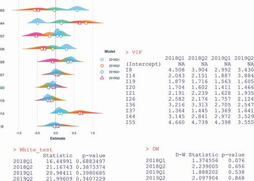
For initial variables, the models are valid, but it is necessary to test other regression hypotheses, like: multicollinearity (that does not represent a problem for principal components), heteroscedasticity or the correlation between the residuals. Figure 6 from above shows the representation of each model’s estimations, the VIF (variance inflation factor), the White’s test and the Durbin-Watson’s test. The results are computed for the first 4 models (2018 and 2019) taking into account the initial variables: the VIF is under 5, so the multicollinearity is moderate, while the p-value for both White and D-W tests are higher than 0.05, as the homoscedasticity is present and the residuals are not correlated.

For 2020 (Q1 and Q2) datasets, it is important to analyze each quarter taking into account the dummy variables and the interactions of dummy variables with the original variables.

Figure 7. Regression models results for 2020 - Q1.

Outputs obtained in R software, t statistic is in parentheses, ***, **, * refers to level of significance: 1%, 5%, 10%

Figure 7 presents the regression models for 2020-Q1 dataset, taking into account the dummy variables (left figure) and the interactions between the dummy variables and the independent variables (right figure). All models are valid and explain a large part of the variance of dependent variable (GDP_gr). The models with interaction variables (right figure) show the influence of the interaction between a dummy variable and an initial indicator to GDP_gr: the close measures analysed here (the require of not leaving house – stay_home, and internal movement restrictions – internal) interact with I21 indicator (taxes on production and imports less subsidies) and show a negative influence for GDP_gr. Countries that implemented these measures more than other countries in the first 3 months of 2020 have a higher decrease in GDP (as change on previous period). The estimated models can be written as:

(3) $GDP\mathrm{\_}gr={\beta }_0+{\beta }_1{I}_8+{\beta }_2{I}_{14}+{\beta }_3{I}_{19}+{\beta }_4{I}_{20}+{\beta }_5{I}_{21}+{\beta }_6{I}_{26}+{\beta }_7{I}_{36}+{\beta }_8{I}_{37}+{\beta }_9{I}_{44}+{\beta }_{10}{I}_{55}+{\beta }_{11}D+\epsilon$(3)

where {school, workplace, stay home, internal, ban_arrivals, cases} represents the dummy variable.

(4) $GD{P}_{gr}={\beta }_0+{\beta }_1{I}_8+{\beta }_2{I}_{14}+{\beta }_3{I}_{19}+{\beta }_4{I}_{20}+{\beta }_5{I}_{21}+{\beta }_6{I}_{26}+{\beta }_7{I}_{36}+{\beta }_8{I}_{37}+{\beta }_9{I}_{44}+{\beta }_{10}{I}_{55}+{\beta }_{11}D+{\beta }_{12}\left(D+I_{21}\right)+\epsilon$(4)

Figure 8. Variance inflation factor, White and Durbin-Watson tests results for 2020-Q1.

Outputs obtained in R software; the Dummy_var $\in \left\{school,workplace,stay\mathrm{\_}home,internal,ban\mathrm{\_}arrivals,cases\right\}$ for each model (example: the name of the model 2020Q1D1 corresponds the first model in Figure 7, where the dummy variable is school)

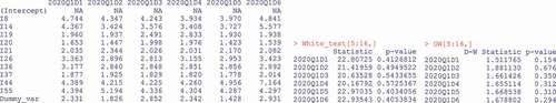
The variance inflation factor, White and Durbin–Watson tests from Figure 8 show the fulfilment of the hypotheses of linear regression. The dummy_var is the dummy variable for each model.

Figure 9. Regression models results for 2020 – Q2.

Outputs obtained in R software, t statistic is in parentheses, ***, **, * refers to level of significance: 1%, 5%, 10%

For 2020-Q2 dataset, the models that present interaction variables between dummy variables and original indicators present interest and are described in Figure 9 from above. The interaction between internal movement restrictions dummy variable and macroeconomic indicators show a small positive impact in GDP_gr by interacting with government consolidated gross debt, a high negative impact in GDP_gr, interacting with the wages and salaries (in agriculture, forestry and fishing), and a moderate negative impact, interacting with real labor productivity per person. Considering the impact of covid-19 virus as the number of cases dummy variable, the interaction with final consumption expenditure of households have a positive impact on GDP_gr, the interaction with the wages and salaries (in industry except construction) have a positive and high influence on GDP_gr, while the interaction with subsidies have a high impact on dependent variable. On the other side, the interaction between work from home measure and final consumption expenditure of households have a positive impact in GDP_gr, while the interaction between the ban arrivals variable and wages and salaries in industry have a significant negative influence on dependent variable.

Figure 10. Regression models results for 2020 – Q2.

Outputs obtained in R software, t statistic is in parentheses, ***, **, * refers to level of significance: 1%, 5%, 10%

The models without the dummy variables or interaction variables for Q1–2020 and Q2–2020 datasets were estimated and presented in Figure 10 from above. The results are similar to datasets from 2018, 2019, and, in this respect, the robustness for regression models is checked.

IV. Conclusion and further research

The main hypothesis that this research relies on is that the pandemic situation had a major impact in the economy field. When the pandemic hit Europe, the governments were forced to take closure measures in order to reduce the spread of the virus, without considering the immediate economic impact. The closure measures adopted also forced governments to take economic decisions to compensate employees who lost their job, or companies that reduced/closed the activity. On short-term, the impact in GDP growth is reduced (by encouraging consumption, for example), but, on long-term, these measures are unsustainable and represent the point of start for an inevitable economic crisis. The main results of this analysis show that GDP is negatively influenced by adopted ‘stay home’ and ‘ban arrivals’ measures and positively by ‘workplace’ measure in 2020-Q1. The workplace measure in 2020-Q2 interacting with the final consumption expenditure of households leads to an increase of GDP.

In this paper, the closure measures were considered as dummy variables and analysed, but, for further research, the economic measures implemented by each country could represent another point of interest. Also, another direction for further research represents the extension of the analysis considering more countries, not only European countries.

Disclosure statement

Nopotential conflict of interest was reported by the author(s).

Notes

1 https://sgp.fas.org/crs/row/R46270.pdf.

References

- Congressional Research Service (CRS) Report: Global Economic Effects of COVID-19, November 2021, accessed January 2022. https://sgp.fas.org/crs/row/R46270.pdf
- Abiad, Abdul et al The Economic Impact of the COVID-19 Outbreak on Developing Asia. 2020. accessed 1 December 2020, [Online] at https://doi.org/http://dx.doi.org/10.22617/BRF200096 doi:https://doi.org/http://dx.doi.org/10.22617/BRF200096
- Atkeson, A. 2020. “What Will Be the Economic Impact of COVID-19 in the US? Rough Estimates of Disease Scenarios.” NBER working paper series, Working Paper 26867, National Bureau of Economic Research Massachusetts Avenue Cambridge, MA. https://www.nber.org/papers/w26867
- Baek, S., and K. Y. Lee. 2021. “The Risk Transmission of COVID-19 in the US Stock Market.” Applied Economics 53 (17): 17, 1976–1990. doi:https://doi.org/10.1080/00036846.2020.1854668.
- Barrett, P., S. Das, G. Magistretti, E. Pugacheva, and P. Wingender. 2021. “After-Effects of the COVID-19 Pandemic: Prospects for Medium-Term Economic Damage.” IMF Working Paper WP/21/203. https://www.imf.org/en/Publications/WP/Issues/2021/07/30/After-Effects-of-the-COVID-19-Pandemic-Prospects-for-Medium-Term-Economic-Damage-462898
- Chen, S., D. O. Igan, N. Pierri, and A. F. Presbitero. 2020. “Tracking the Economic Impact of COVID-19 and Mitigation Policies in Europe and the United States.” IMF Working Papers, 2020/125. International Monetary Fund, https://doi.org/10.5089/9781513549644.001
- Chen, H., W. Qian, and Q. Wen. 2020. “The Impact of the COVID-19 Pandemic on Consumption: Learning from High Frequency Transaction Data.” July 1. Available at SSRN. https://ssrn.com/abstract=3568574 or https://doi.org/http://dx.doi.org/10.2139/ssrn.3568574
- Chen, L., D. Raitzer, R. Hasan, R. Lavado, and O. Velarde. 2020. “What Works to Control COVID-19? Econometric Analysis of a Cross-Country Panel.” Asian Development Bank Economics Working Paper Series, No. 625. December 4 . Available at SSRN: https://ssrn.com/abstract=3785083
- Corbet, S., Y. G. Hou, and Y. Hu., L. Oxley. 2021. “Financial Contagion Among COVID-19 Concept-Related Stocks in China.” Applied Economics 1–14. doi:https://doi.org/10.1080/00036846.2021.1990844.
- de la Fuente-Mella, H., R. Rubilar, K. Chahuán-Jiménez, and V. Leiva. 2021. “Modeling COVID-19 Cases Statistically and Evaluating Their Effect on the Economy of Countries.” Mathematics 9 (13): 1558. doi:https://doi.org/10.3390/math9131558.
- European Centre for Disease Prevention and Control. accessed 1 December 2020 . [Online]. https://www.ecdc.europa.eu/en/publications-data/download-todays-data-geographic-distribution-covid-19-cases-worldwide
- European Statistical Recovery Dashboard. 2021. accessed 1 December 2020, [Online] at https://ec.europa.eu/eurostat/data/database
- Farzanegan, M. R., F. Mehdi, and F. G. Hassan. 2021. “Globalization and the Outbreak of COVID-19: An Empirical Analysis.” Journal of Risk and Financial Management 14 (3): 105. doi:https://doi.org/10.3390/jrfm14030105.
- Fernandes, N. 2020. “Economic Effects of Coronavirus Outbreak (COVID-19) on the World Economy.” IESE Business School Working Paper, No. WP-1240-E, [Online]. https://ssrn.com/abstract=3557504
- Gandjour, A. 2020. “The Clinical and Economic Value of a Successful Shutdown During the SARS-CoV-2 Pandemic in Germany.” The Quarterly Review of Economics and Finance 2020. doi:https://doi.org/10.1016/j.qref.2020.10.007.
- Gunay, S., G. Can, and M. Ocak 2021. ”Forecast of China’s Economic Growth During the COVID-19 Pandemic: A MIDAS Regression Analysis.” Journal of Chinese Economic and Foreign Trade Studies 14 (1): 3–17. https://doi.org/10.1108/JCEFTS-08-2020-0053.
- Hale, T., N. Angrist, R. Goldszmidt, B. Kira, A. Petherick, T. Phillips, S. Webster, et al. 2021. “A Global Panel Database of Pandemic Policies (Oxford COVID-19 Government Response Tracker).” Nature Human Behaviour 5 (4): 529–538. doi:https://doi.org/https://doi.org/10.1038/s41562-021-01079-8.
- Hlavac, M. 2018. “Stargazer: Well-Formatted Regression and Summary Statistics Tables.” R package version 5.2.2. https://CRAN.R-project.org/package=stargazer
- Jayaram, K., A. Leke, A. Ooko-Ombaka, and Y. S. Sun 2020. “Tackling COVID-19 in Africa.” McKinsey & Company, April.
- Keogh-Brown, M. R., H. T. Jensen, W. J. Edmunds, and R.D. Smith 2020. ”The Impact of Covid-19, Associated Behaviors and Policies on the UK Economy: A Computable General Equilibrium Model.” SSM - Population Health 12: 100651 . [Online] at doi:https://doi.org/https://doi.org/10.1016/j.ssmph.2020.100651.
- Konig, M., A. Winkler, and B. Xue. 2021. “The Impact of Government Responses to the COVID-19 Pandemic on GDP Growth: Does Strategy Matter?” PLoS One 16 (11): e0259362. doi:https://doi.org/10.1371/journal.pone.0259362.
- Makridis, C., and J. Hartley 2020. ”The Cost of COVID-19: A Rough Estimate of the 2020 US GDP Impact.” SpSpecial Edition Policy Brief. doi:https://doi.org/http://dx.doi.org/10.2139/ssrn.3570731.
- Mariolis, T., N. Rodousakis, and G. Soklis. 2020. “The COVID-19 Multiplier Effects of Tourism on the Greek Economy.” Tourism Economics. doi:https://doi.org/10.1177/1354816620946547.
- Martin, A., M. Markhvida, S. Hallegatte, and B. Walsh. 2020. “Socio-Economic Impacts of COVID-19 on Household Consumption and Poverty.” Economics of Disasters and Climate Change 4 (3): 453–479. doi:https://doi.org/https://doi.org/10.1007/s41885-020-00070-3.
- McKibbin, W., and R. Fernando (2020a), “The economic impact of COVID-19. Economics in the Time of COVID-19,” Centre for Economic Policy Research, London, UK.
- McKibbin, W. J., and R. Fernando. 2020b. “The Global Macroeconomic Impacts of COVID-19: Seven Scenarios.” CAMA Working Paper, No. 19, [Online] at https://ssrn.com/abstract=3547729 or https://doi.org/http://dx.doi.org/10.2139/ssrn.3547729
- Meinen, P., R. Serafini, and O. Papagalli. 2021. “Regional Economic Impact of COVID-19: The Role of Sectoral Structure and Trade Linkages.” ECB Working Paper No. 2021/2528, February 1. https://ssrn.com/abstract=3797148
- Mitleton-Kelly, E. 2003. “Ten principles of complexity and enabling infrastructures.” Elsevier
- Pasaribu, E., T. Siagian, I. Wulansari, P. Irawan, and R. Kurniawan 2021, “Spillover Effects of Social and Economic Interactions on COVID-19 Pandemic Vulnerability Across Indonesia’s Regions”, available at: https://www.eria.org/publications/spillover-effects-of-social-and-economic-interactions-on-covid-19-pandemic-vulnerability-across-indonesias-regions/
- Principal component regression. 2020. accessed 1 December 2020. [Online] at https://en.wikipedia.org/wiki/Principal_component_regression
- Putra, R. A. A., and S. F. Arini 2020. “Measuring the Economics of a Pandemic: How People Mobility Depict Economics? an Evidence of People’s Mobility Data Towards Economic Activities.” Randra Putra, Silvia Arini, accessed January 2022: https://www.imf.org/-/media/Files/Conferences/2020/8th-stats-forum/paper-rendra-putra-and-silvia-arini.ashx
- Solihin, A., W. W. Wardana, E. Fiddin, N. M. Sukartini, and R. Read. 2021. “Do Government Policies Drive Economic Growth Convergence? Evidence from East Java, Indonesia.” Cogent Economics & Finance 9 (1): 1992875. doi:https://doi.org/10.1080/23322039.2021.1992875.
- Tchatoka, F. D., J. Julia Puellbeck, and V. Masson. 2022. “Stock Returns in the Time of COVID-19 Pandemic.” Applied Economics. doi:https://doi.org/10.1080/00036846.2021.1975028.