Gender and gambling preference

ABSTRACT

Gambling preferences are analysed using survey data from the wider population. Respondents were confronted with a hypothetical lottery question, in which they were asked to imagine having just won a large prize, and asked how much of this prize they would be willing to invest in a further gamble. We observe the majority of respondents avoiding the gamble altogether. We demonstrate that such behaviour cannot easily be explained by standard models of choice under risk, since it implies implausible degrees of risk aversion. We propose that the observed behaviour can instead be explained in terms of gambling aversion. Since the decision variable takes the form of the number of ‘units’ of the prize that the respondent wishes to invest in the gamble, and since the decision is observed twice for some respondents, we adopt the panel version of the Zero-Inflated Poisson model as an econometric framework. We assume that individual characteristics affect both stages of the decision-making process. We are particularly interested in the effect of gender, and we find that males have a significantly higher probability of participating in the gamble, and are also (conditional on gambling) prepared to gamble significantly larger amounts.

KEYWORDS:

• Gambling behaviour
• gender
• panel zero-inflated Poisson model
• survey data

JEL CLASSIFICATION:

• C 33
• D01
• J16

I. Introduction

An understanding of gambling preference is critical in tackling the social issue of ‘problem gambling’ (Meyer, Hayer, and Griffiths 2009; Ring et al. 2022), and also because it plays an important role in certain models in Financial Economics (see e.g. Doran, Jiang, and Peterson 2012). Empirical research on the determinants of gambling preference often focuses on problem gamblers (LaPlante et al. 2006; Odlaug et al. 2011; Sancho et al. 2019). However, problem gamblers are known to comprise a very small proportion of the overall population,¹ and hence using such data sources clearly requires adjustments for sample selection. This paper avoids such selection issues by using survey data from the wider population. Another problem associated with surveys targeted at problem gamblers is that such individuals have a tendency to lie when responding to questions relating directly to problem gambling (Johnson, Hamer, and Nora 1998) and this brings into question the validity of the data. In this paper we avoid this problem by analysing survey questions that are not directly posed for the purpose of uncovering problem gambling.

We are particularly interested in the effect of gender on gambling preference. The key questions we aim to answer are which gender is more likely to gamble, and which gender gambles larger amounts. Note that the answers to these two questions are not necessarily the same. The survey response on which we focus is a hypothetical lottery question with high stakes. Survey questions of this type have been useful in estimating the risk attitudes of respondents (see e.g. Bacon, Conte, and Moffatt 2020). However, such survey questions tend to produce choices that imply implausibly high levels of risk aversion. In this paper, we postulate that, when an individual is faced with a high-stakes lottery, ‘gambling preference’ takes precedence over risk preference in determining such choices. In particular, the high incidence of the choice of the safest alternative may be attributed to a form of ‘gambling aversion’.

The difference between gambling aversion and risk aversion may be viewed as a framing issue. A given risky choice problem may be framed as either an investment or a gamble (see Shang, Duan, and Lu 2021). If the problem is framed as an investment, it might be presented to subjects using words such as ‘business venture’, ‘profit’, ‘investment opportunity’, ‘returns’. We hypothesize that this framing is likely to result in decisions that are easily explained by conventionally assumed levels of risk aversion. Alternatively, the same risky choice problem could be framed as an out-and-out gamble, using words such as ‘lottery’, ‘stake’, and ‘winnings’, and we hypothesize that this framing induces gambling aversion, causing a higher proportion of individuals to be drawn to the safer (or safest) alternative. The risky choice problem that we analyse is indeed framed as a gamble, since instructions to the participant include these three words.

An understanding of the difference between gambling aversion and risk aversion is particularly important at the present time, since there is currently a sense that the distinction between some forms of financial market trading and more traditional forms of gambling has recently become blurred. A stark example of this phenomenon is the rapid expansion of crypto-currency trading in the last decade. A recent literature has emerged that identifies a link between crypto-trading and increased rates of problem gambling (see e.g. Delfabbro, King, and Williams 2021). One key concept in this literature is the ‘illusion of control’: for various reasons, crypto-traders may develop a belief that their trading decisions are based on forms of financially sound reasoning, thereby constituting a financially healthy activity, while in truth they are no different, in essence, from conventional forms of gambling. Such traders are in a sense impervious to gambling aversion simply because they do not perceive their own activities as gambling.

The role of gender in the context of gambling preference may be analysed in the framework of a theoretical model of behaviour under risk. Sitkin and Pablo (1992) have argued that individual characteristics (including gender) and problem-related characteristics (e.g. framing) do not influence risk behaviour directly, but only indirectly, via the mediating mechanisms of risk perception and risk propensity. Risk perception is the decision-maker’s assessment of the risk inherent in a given situation, and is influenced, among other things, by problem framing.² Risk propensity is determined by individual risk preferences, inertia (or habit formation), and outcome history (i.e. previous experience in risk-taking). Thus we see that there are two distinct channels through which gender may ultimately influence behaviour in the present context: through its impact on risk perception, in terms of males and females reacting differently to the gambling frame; and through its effect on risk propensity which is in turn determined by lifetime experience, and of course we expect to see systematic gender-differences in lifetime experience.

We use the same hypothetical lottery choice data used by Bacon, Conte, and Moffatt (2020), from the German Socio-Economic Panel Survey (SOEP), but we shift the focus from risk preference to gambling preference. The hypothetical question analysed places respondents in the imaginary scenario of having just won a large sum of money, and the question essentially asks how much of the prize that they have just won, they are willing to risk in a further gamble.

Hence the setting bears similarities to some settings that have been studied in the gambling addiction literature. For example, in the context of scratch card gambling, Griffiths (1995) finds evidence that receiving winnings acts as a reinforcement to winners to continue gambling, and further notes that the industry exploits this by ensuring that winnings can be gambled immediately. We are particularly interested in this concept of reinforcement. In our context, as already noted, a significant proportion of the sample avoid the gamble, but some do gamble to varying degrees, and this may be partly explained in terms of reinforcement brought about by the large (hypothetical) win.

Since our survey question essentially asks the respondent how many units of €20,000 they would gamble having just won €100,000, we treat the response as a count variable, and apply models appropriate for count data, namely the Poisson regression model. Count data models have been used previously in gambling research by Kastirke et al. (2015). Moreover, in recognition that a proportion of the population are ‘gambling averse’, we adopt a zero-inflated version of the Poisson model (ZIP) (Lambert 1992), in order to separate out the effects of individual characteristics on participation in gambling and the extent of the gamble. Actually, since some respondents are observed on more than one occasion, we use the panel-data extension of the ZIP model (Wang, Yau, and Lee 2002). Similar models have been used previously in gambling research. For example, Jaunky and Ramchurn (2014) apply a double-hurdle model to scratch card purchases, and find interestingly that while males are less likely to participate than females, participating males tend to spend more than participating females.

There is some evidence on the effect of gender on risk-taking more generally. Dohmen et al. (2011, 535) find that males are significantly more willing to take risks than females and that this difference is most pronounced in the domain of financial risk taking. Halko, Kaustia, and Alanko (2012) analyse data from a context-specific cohort of Finnish investors who were given hypothetical investment questions similar to the one we analyse. They find that females are more risk averse but the difference is not statistically significant. Welte et al. (2007) provide interesting evidence on the types of gambling that present the most severe problems for each gender. For males, the problem types are casinos and card games; for females, they are lotteries, casinos, gambling machines and bingo.

The objective of this paper is to estimate the effects of respondent characteristics including gender on both participation and extent of the gamble, using the aforementioned hypothetical response data from a large survey of the wider population.

The paper is structured as follows. Section II describes the data set, Section III describes the model, Section IV presents the results, and Section V concludes.

II. Data description

The data set used in this study is extracted from the German Socio-Economic Panel Survey (SOEP) (Wagner, Burkhauser, and Behringer 1993; Wagner, Frick, and Schupp 2007). This is a representative panel survey of the resident adult population of Germany surveying approximately 20,000 households annually, and inquiring into lifestyle and economic activities. It has been running since 1984. In 2004, the survey broadened to include questions associated with risk attitude.

The question on which we focus is the ‘hypothetical lottery question’. This question was asked in two years of the survey, 2004 and 2009. It takes the following form:

Imagine that you have won €100,000 in the lottery. Immediately after receiving your winnings you receive the following offer: You have the chance to double your money. But it is equally possible that you will lose half the amount invested. You can participate by staking all or part of your €100,000 on the lottery, or choose not to participate at all. What portion of your lottery winnings are you prepared to stake on this financially risky, yet potentially lucrative lottery investment?

€100,000 (i.e. all of it);

€80,000;

€60,000;

€40,000;

€20,000;

Nothing: I would decline the offer

Data on responses to this hypothetical lottery question form the focus of our model of gambling preference which is described in Section III. From the SOEP data we also extract a number of demographic variables which are used as explanatory variables in the model. These include gender, age, marital status, and years of education. Descriptive statistics of all variables used, along with SOEP dataset codes, are supplied in Table A1 of the Appendix. There, we see that the data set consists of 27,474 respondents, of whom 48% are male, and with average age 48.8.

The 27,474 respondents generate 41,704 observations; 14,230 respondents are observed in both years, 7,025 in 2004 only and 6,219 in 2009 only. Of those who are observed in both years, 8,182 (57.5%) choose the same investment both times, 4,252 (29.9%) invested less in 2009 than they did in 2004, 1,796 (12.6%) invested more in 2009. This amounts to strong evidence that investments were lower in 2009 (Wilcoxon signed-rank test: $z=31.523$, $p$-value = 0.0000). Bacon, Conte, and Moffatt (2020) explain this change in terms of risk vulnerability (Gollier and Pratt 1996). Specifically, agents are more risk averse at times of high background risk, as was the case in 2009, being the nadir of the global recession that followed the global financial crisis.

In Table A1 of the Appendix, we see that the mean number of coupons invested in 2004 and 2009 are 0.71 and 0.46 respectively. It is useful to compare these to the two variances, which are 1.17 and 0.98 respectively. We therefore see that the variance is somewhat higher than the mean in both years, implying overdispersion. This is a well-known feature of count data, which essentially indicates that the simple Poisson model is inappropriate as a modelling framework. One common cause of overdispersion is the presence of excess zeros (Winkelmann 2008). It is therefore not surprising that the overdispersion (measured as the variance-mean ratio) appears to be higher in the year 2009, when, as seen clearly in Figure 1, excess zeros were more prominent. The clear presence of excess zeros, and consequent overdispersion, is one of the important data features that guides our choice of econometric modelling strategy.

Figure 1. Distribution of response to hypothetical lottery question by year and gender.

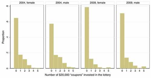
In Figure 1 we also see evidence that males are less likely than females to choose a zero investment, and that positive investments tend to be higher for males. Note that these two observations provide a non-parametric preview of the key results we will be looking for in the parametric model.

Bacon, Conte, and Moffatt (2020) have used the same data set to estimate the distribution of risk aversion over the population. They derive ranges of absolute risk aversion corresponding to each choice. For example, they find that, under the assumption of expected utility maximization, the choice to gamble zero implies a coefficient of absolute risk aversion greater than 4.70. It may be seen as implausible that the majority of the population are this risk averse, not least because it is so at-odds with estimates of risk aversion estimated in other contexts in previous literature.³ For this reason we propose that behaviour in large-stakes hypothetical lotteries may be better modelled in terms of gambling preference rather than risk preference. In particular, we hypothesize that the decision to gamble zero is the result of an aversion to any sort of gamble rather than that of very high risk aversion.

III. Econometric model

For the purpose of our econometric model of gambling preference, we imagine that, when faced with the hypothetical lottery question described in Section II, an individual is endowed with five ‘coupons’ worth €$20,000$ each, and their choice problem amounts to deciding how many of these five ‘coupons’, if any, to invest in the gamble.⁴ Accordingly we define the dependent variable $y_{it}$ for subject $i$, $i=1,\dots ,n$, in period $t\in \left\{2004,2009\right\}$, as the number of coupons invested, so that $y_{it}\in \left\{0,1,\dots ,5\right\}$. Hence we treat $y_{it}$ as a count variable, and model it as such.

Some respondents choosing to invest zero may be labelled as gambling-averse. For those who choose to invest, the number of coupons invested may be interpreted as the level of affinity towards this particular gamble. Of course, an investment of zero does not imply gambling aversion, because the zero investment may be a result of low affinity towards the gamble. Hence there are two types of zero: gambling aversion, and low affinity. Respondents appearing in the right tail of the distributions in Figure 1 have the highest affinity towards the gamble. In order to capture the concepts of both gambling-aversion and affinity towards the gamble, a two-part econometric model is required, with one equation representing the decision to participate in the gamble, and the other representing the level of investment. Note that affinity towards the gamble, represented by the second of these two equations, is closely related to the phenomenon of reinforcement Griffiths 1995 that was discussed in Section 1 in the context of scratchcard gambling. Here, we perceive a high investment as a manifestation of reinforcement: the individual is being lured by the experience of the windfall gain into risking a high proportion of the gain in a further gamble.

The random-effects zero-inflated Poisson model

We model this situation via a random-effects zero-inflated Poisson model (see Crepon and Duguet 1997; Wang, Yau, and Lee 2002; Song et al. 2018).⁵

Let $p_{it}$ be the probability of being a gambler in period $t$, and, consequently, $\left(1-p_{it}\right)$ captures the probability of those who are not likely to engage in gambling activities in the current circumstances. Then, the probability of observing $y_{it}=k$ for subject $i$ in period $t$ is:

(1) $f\left(y_{it};p_{it},{\lambda }_{it}\right)=\left\{\begin{array}{cc}\left(1-p_{it}\right)+p_{it}\mathcal{P}\left(0;{\lambda }_{it}\right)& \mathrm{i}\mathrm{f}k=0\\ p_{it}\mathcal{P}\left(y_{it};{\lambda }_{it}\right)& \mathrm{i}\mathrm{f}k=1,\dots ,5\end{array}\right.$(1)

Here, $\mathcal{P}\left(k;{\lambda }_{it}\right)$ is the Poisson probability mass function evaluated at $k$, with parameter ${\lambda }_{it}>0$. Disregarding $t$, this model is a zero-inflated Poisson model (Lambert 1992). The idea behind it is that each subject’s decision can be regarded as a draw from a Poisson distribution with an abnormal mass at zero. With probability $\left(1-p_{it}\right)$, the subject is a non-gambler and falls in the excess mass at zero of the distribution; with probability $p_{it}$, the subject’s decision is driven from a standard Poisson distribution, that is they can decide to invest any number of coupons from the amount previously won. This number includes zero, given that they might be gamblers but unwilling to invest in this particular lottery.

We said that we distinguish between gamblers and non-gamblers in the current circumstances. In some sense, we need to control for those who do not gamble in order to be able to identify the features of those who are prone to gambling addiction, that we identify as those who are in the upper tail of the Poisson distribution. The probability of being a gambler, $p_{it}$, is modelled via a normal probability distribution function, $\mathrm{\Phi }\left(.\right)$, and depends on the vector of individual characteristics (including an intercept) intended to capture the ‘current circumstances’, $x_{it}$, in the following way:

(2) $p_{it}=\mathrm{\Phi }\left({x{ }^{\mathrm{\prime }}}_{it}\gamma +{\delta }_i\right)$(2)

Here, $\gamma$ is a vector of coefficients on the variables in $x_{it}$ to be estimated and ${\delta }_i$ is an individual-specific intercept. Basically, this component of the model is similar to a probit model. If a subject is a non-gambler, based on the current circumstances, they should score a zero and contribute to the observed mass at zero. Otherwise, they are a gambler and decide on an amount (taken from the amount previously won) to invest in the proposed lottery.

The intensity of the attitude to gambling, signalled by the number of €20,000 notes invested, depends on the parameter ${\lambda }_{it}$ according to some individual characteristics, subsumed by the vector $x_{it}$,⁶ and an individual-specific term ${\alpha }_i$ as follows:

(3) ${\lambda }_{it}=exp\left({x{ }^{\mathrm{\prime }}}_{it}\beta +{\alpha }_i\right)$(3)

where $\beta$ is a vector of coefficients to be estimated.

We assume that the two individual-specific random variables ${\alpha }_i$ and ${\delta }_i$ follow a bivariate normal distribution:

(4) $\left(\begin{array}{c}{\alpha }_i\\ {\delta }_i\end{array}\right)\sim N\left(\begin{array}{c}\left(\begin{array}{c}0\\ 0\end{array}\right),\left(\begin{array}{c}{\sigma }_{\alpha }^2,\rho {\sigma }_{\alpha }{\sigma }_{\delta }\\ \rho {\sigma }_{\alpha }{\sigma }_{\delta },{\sigma }_{\delta }^2\end{array}\right)\end{array}\right)$(4)

where $\sigma$ represents the standard deviations and $\rho$ the correlation.

The probability of observing $y_{it}=k$ is

(5) $\begin{array}{rl}& Pr\left(y_{it}=k|{\alpha }_i,{\delta }_i\right)={\left\{\left[1-\mathrm{\Phi }\left({x{ }^{\mathrm{\prime }}}_{it}\gamma +{\delta }_i\right)\right]\text{break}+\mathrm{\Phi }\left[{x{ }^{\mathrm{\prime }}}_{it}\gamma +{\delta }_i\right]\times \mathcal{P}\left(0;{x{ }^{\mathrm{\prime }}}_{it}\beta +{\alpha }_i\right)\right\}}^{\mathbf{1}\left[y_{it}=0\right]}+{\left\{\mathrm{\Phi }\left[{x\prime }_{it}\gamma +{\delta }_i\right]\times \mathcal{P}\left(k;{x\prime }_{it}\beta +{\alpha }_i\right)\right\}}^{\mathbf{1}\left[y_{it}\ne 0\right]}\end{array}$(5)

Assuming that, conditional on ${\alpha }_i$ and ${\delta }_i$, the probability of observing a certain outcome is independent over individual-specific random variables and everything else in the model, we can write the individual likelihood contribution for subject $i$ observed in the two periods $t=1,2$ as:

(6) $\begin{array}{rl}& Pr\left(y_{i1},y_{i2}|{\alpha }_i,{\delta }_i\right)=\prod _{t=1,2}\{{\left\{\left[1-\mathrm{\Phi }\left({x{ }^{\mathrm{\prime }}}_{it}\gamma +{\delta }_i\right)\right]\text{break}+\mathrm{\Phi }\left[{x{ }^{\mathrm{\prime }}}_{it}\gamma +{\delta }_i\right]\times \mathcal{P}\left(0;exp\left({x{ }^{\mathrm{\prime }}}_{it}\beta +{\alpha }_i\right)\right)\right\}}^{\mathbf{1}\left[y_{it}=0\right]}+{\left\{\mathrm{\Phi }\left[{x{ }^{\mathrm{\prime }}}_{it}\gamma +{\delta }_i\right]\times \mathcal{P}\left(y_{it};exp\left({x{ }^{\mathrm{\prime }}}_{it}\beta +{\alpha }_i\right)\right)\right\}}^{\mathbf{1}\left[y_{it}\ne 0\right]}\end{array}$(6)

By integrating out ${\alpha }_i$ and ${\delta }_i$, we obtain the unconditional individual likelihood contribution as:

(7) $Pr\left(y_{i1},y_{i2}\right)={\int }_{-\mathrm{\infty }}^{\mathrm{\infty }}{\int }_{-\mathrm{\infty }}^{\mathrm{\infty }}Pr\left(y_{i1},y_{i2}|\alpha ,\delta \right)g\left(\alpha ,\delta \right)d\alpha d\delta$(7)

where $g\left(a,b\right)$ is the bivariate normal density function evaluated at $a$ and $b$.

The full-sample log-likelihood for the sample of individuals in the two periods is

(8) $\mathrm{L}\mathrm{o}\mathrm{g}-\mathrm{L}\mathrm{i}\mathrm{k}\mathrm{e}\mathrm{l}\mathrm{i}\mathrm{h}\mathrm{o}\mathrm{o}\mathrm{d}=\sum _{i=1}^{n}logPr\left(y_{i1},y_{i2}\right)$(8)

IV. Estimation results

The model is estimated using data from the full sample with a gender dummy (1 for male; 0 for female) which is also interacted with all the other regressors. To estimate the model, we use the method of Maximum Simulated Likelihood. The double integral appearing in (7) is evaluated using two sets of Halton sequences (100 draws per subject).

For the sake of checking the robustness of our main results, we estimate three different specifications of the model. Table 1 presents the results for specification 1. This includes basic characteristics of the individual and also a dummy for the second survey year 2009. Table 2 presents the results for specification 2 which adds a control for risk-lovingness to specification 1.⁷ Table 3 shows the results for specification 3 which adds a set of self-reported life-satisfaction variables (all in binary form) to specification 1. Results in the tables are displayed in two main columns: one, labelled ‘Participation’, relates to the probability ($p_{it}$ defined in (2)) of participating in the gamble under the prevailing circumstances captured by the explanatory variables; the other, labelled ‘Investment’, shows the factors that influence the amount invested ($log\left({\lambda }_{it}\right)$ defined in (3)) measured in number of €20,000 ‘coupons’. The same explanatory variables are used to explain both participation and investment. For each of these, the corresponding coefficients for male and female are deduced, with standard errors are obtained via the delta method. In the tables, for both the participation and the investment equations, we report coefficient estimates for male and female and also the male-female difference (again with standard errors obtained using the delta method) to ease inter-gender comparisons.

Table 1. Estimation results (specification 1).

	PARTICIPATION ($p_{it}$)			INVESTMENT ($log\left({\lambda }_{it}\right)$)
$Regressors$	male	female	difference	male	female	difference
year 2009	−0.641***	−0.813***	0.172***	−0.038	−0.050*	0.012
	(0.043)	(0.050)	(0.057)	(0.024)	(0.030)	(0.038)
age	−0.020***	−0.024***	0.004	−0.003***	0.001	−0.005**
	(0.002)	(0.002)	(0.003)	(0.001)	(0.001)	(0.002)
married	−0.102	−0.250***	0.147	−0.088**	−0.115**	0.027
	(0.071)	(0.069)	(0.106)	(0.041)	(0.048)	(0.063)
separated	0.004	0.500**	−0.497*	0.012	−0.166	0.179
	(0.155)	(0.214)	(0.264)	(0.092)	(0.110)	(0.143)
divorced	0.052	−0.164	0.216	−0.072	−0.066	−0.006
	(0.099)	(0.100)	(0.141)	(0.060)	(0.067)	(0.090)
widowed	−0.080	−0.099	0.019	0.034	0.062	−0.028
	(0.141)	(0.111)	(0.179)	(0.105)	(0.081)	(0.133)
# children in HH	−0.016	−0.079***	0.063	0.013	0.005	0.008
	(0.027)	(0.030)	(0.041)	(0.015)	(0.019)	(0.024)
years of education	0.059***	0.076***	−0.017*	0.015***	−0.005	0.020***
	(0.007)	(0.008)	(0.010)	(0.004)	(0.005)	(0.006)
log net HH income	0.225***	0.236***	−0.007	0.077***	0.014	0.064**
	(0.026)	(0.037)	(0.051)	(0.020)	(0.023)	(0.030)
employed	0.067	0.047	0.020	0.001	0.022	−0.020
	(0.051)	(0.053)	0.073	(0.031)	(0.034)	(0.046)
home owner	0.167***	0.174***	−0.007	−0.080***	−0.116***	0.036
	(0.047)	(0.051)	(0.069)	(0.029)	(0.035)	(0.046)
constant	−1.866***	−1.877***	0.010	−0.531**	−0.073	−0.457
	(0.363)	(0.383)	(0.523)	(0.212)	(0.239)	(0.317)
${\sigma }_{\delta }$	0.970***
	(0.063)
${\sigma }_{\alpha }$	0.350***
	(0.018)
$\rho$	0.373***
	(0.117)
Log-likelihood	−40678.73
# observations	41,695
# subjects	27,474

For both the “participation” and “investment” equations, the three columns report the estimated coefficients on the explanatory variables in the first column for male, female and the difference between the two coefficients (male-female). Standard errors are reported in parentheses. *, **, *** indicate a -value , and , respectively. The joint equality of male and female coefficients is tested via a Wald test for the “participation” equation (, -value=0.000), the “investment” equation (, -value=0.000) and the whole model (, -value=0.000).

Table 2. Estimation results (specification 2).

	PARTICIPATION ($p_{it}$)			INVESTMENT ($log\left({\lambda }_{it}\right)$)
$Regressors$	male	female	difference	male	female	difference
year 2009	−0.622***	−0.802***	0.180***	0.008	−0.011	0.020
	(0.044)	(0.049)	(0.057)	(0.024)	(0.030)	(0.038)
age	−0.019***	−0.024***	0.005	−0.001	0.003*	−0.004**
	(0.002)	(0.002)	(0.003)	(0.001)	(0.001)	(0.002)
married	−0.082	−0.239***	0.156	−0.078*	−0.090*	0.011
	(0.071)	(0.077)	(0.105)	(0.040)	(0.047)	(0.062)
separated	0.014	0.489**	−0.475*	−0.002	−0.167	0.166
	(0.157)	(0.208)	(0.260)	(0.089)	(0.108)	(0.140)
divorced	0.059	−0.148	0.207	−0.094	−0.058	−0.036
	(0.100)	(0.098)	(0.140)	(0.058)	(0.065)	(0.087)
widowed	−0.085	−0.082	−0.003	0.071	0.052	0.019
	(0.139)	(0.109)	(0.176)	(0.103)	(0.079)	(0.130)
# children in HH	−0.016	−0.077***	0.061	0.018	0.011	0.006
	(0.027)	(0.030)	(0.040)	(0.015)	(0.018)	(0.024)
years of education	0.052***	0.074***	−0.022**	0.010**	−0.006	0.015***
	(0.007)	(0.008)	(0.010)	(0.004)	(0.005)	(0.006)
log net HH income	0.200***	0.234***	−0.034	0.038*	−0.008	0.047
	(0.036)	(0.037)	(0.050)	(0.020)	(0.022)	(0.030)
employed	0.068	0.042	0.026	−0.004	0.020	−0.024
	(0.050)	(0.051)	0.072	(0.030)	(0.033)	(0.044)
home owner	0.167***	0.174***	−0.008	−0.101***	−0.124***	0.023
	(0.048)	(0.050)	(0.069)	(0.029)	(0.034)	(0.044)
risk loving	0.617***	0.489***	0.127*	0.434***	0.433***	0.001
	(0.049)	(0.058)	(0.073)	(0.024)	(0.031)	(0.039)
constant	−1.732***	−1.968***	0.236	−0.271	0.058	−0.328
	(0.362)	(0.375)	(0.517)	(0.206)	(0.233)	(0.308)
${\sigma }_{\delta }$	0.946***
	(0.063)
${\sigma }_{\alpha }$	0.282***
	(0.020)
$\rho$	0.311***
	(0.143)
Log-likelihood	−40007.96
# observations	41,695
# subjects	27,474

For both the “participation” and “investment” equations, the three columns report the estimated coefficients on the explanatory variables in the first column for male, female and the difference between the two coefficients (male-female). Standard errors are reported in parentheses. *, **, *** indicate a $p$-value $<0.10$, $<0.05$ and $<0.01$, respectively. The joint equality of male and female coefficients is tested via a Wald test for the “participation” equation (${\chi }^2(13)=49.57$, $p$-value=0.000), the “investment” equation (${\chi }^2(13)=110.41$, $p$-value=0.000) and the whole model (${\chi }^2(26)=220.89$, $p$-value=0.000).

Table 3. Estimation results (specification 3).

	PARTICIPATION ($p_{it}$)			INVESTMENT ($log\left({\lambda }_{it}\right)$)
$Regressors$	male	female	difference	male	female	difference
year 2009	−0.645***	−0.828***	0.182***	−0.029	−0.044	0.016
	(0.048)	(0.056)	(0.061)	(0.026)	(0.033)	(0.040)
age	−0.019***	−0.023***	0.004	−0.003**	0.002	−0.005**
	(0.002)	(0.002)	(0.003)	(0.001)	(0.002)	(0.002)
married	−0.091	−0.253***	0.162	−0.075*	−0.098**	0.022
	(0.075)	(0.082)	(0.111)	(0.043)	(0.050)	(0.066)
separated	0.132	0.502**	−0.370*	−0.005	−0.135	0.130
	(0.166)	(0.213)	(0.270)	(0.094)	(0.112)	(0.146)
divorced	0.081	−0.185*	0.266*	−0.056	−0.040	−0.016
	(0.104)	(0.105)	(0.148)	(0.062)	(0.069)	(0.093)
widowed	−0.045	−0.120	0.076	0.026	0.069	−0.043
	(0.149)	(0.117)	(0.190)	(0.108)	(0.084)	(0.137)
# children in HH	−0.004	−0.068*	0.064	0.023	−0.002	0.026
	(0.030)	(0.035)	(0.046)	(0.017)	(0.021)	(0.027)
years of education	0.058***	0.073***	−0.015	0.012***	−0.008	0.020***
	(0.008)	(0.009)	(0.011)	(0.004)	(0.005)	(0.006)
log net HH income	0.170***	0.186***	−0.015	0.089***	0.018	0.070**
	(0.041)	(0.042)	(0.057)	(0.023)	(0.025)	(0.034)
employed	0.059	0.030	0.029	0.014	0.057	−0.043
	(0.063)	(0.067)	0.092	(0.038)	(0.041)	(0.056)
home owner	0.162***	0.135**	0.027	−0.075**	−0.101***	0.026
	(0.050)	(0.054)	(0.063)	(0.030)	(0.036)	(0.047)
satisfied with health	0.062	0.101*	−0.040	−0.026	0.036	−0.061
	(0.053)	(0.055)	(0.058)	(0.033)	(0.039)	(0.051)
satisfied with work	−0.103*	0.009	−0.112	0.030	−0.020	0.050
	(0.057)	(0.064)	(0.086)	(0.033)	(0.039)	(0.051)
satisfied with housework	−0.095**	−0.028**	−0.067	−0.011	−0.064*	0.053*
	(0.043)	(0.052)	(0.067)	(0.026)	(0.033)	(0.042)
satisfied with HH income	0.107**	0.133**	−0.026	−0.022	−0.037	0.015
	(0.054)	(0.058)	(0.079)	(0.033)	(0.038)	(0.051)
satisfied with dwelling	0.019	0.113	−0.132	−0.126***	−0.126***	−0.012**
	(0.068)	(0.072)	(0.099)	(0.041)	(0.049)	(0.048)
satisfied with leisure	0.050	0.030	0.020	−0.093***	−0.081**	−0.082**
	(0.052)	(0.059)	(0.078)	(0.030)	(0.038)	(0.039)
satisfied with childcare	−0.055	−0.086	0.031	−0.069*	−0.044	−0.025
	(0.076)	(0.085)	(0.114)	(0.042)	(0.052)	(0.067)
satisfied with life in 5 years	0.288***	0.189***	0.099	0.124***	0.070	0.053
	(0.057)	(0.062)	(0.083)	(0.038)	(0.045)	(0.059)
worried about finance	−0.053	−0.031	−0.021	−0.033	−0.059	0.026
	(0.053)	(0.059)	(0.079)	(0.031)	(0.037)	(0.049)
worried about job	0.141***	0.011	0.129	−0.111***	−0.078**	−0.032***
	(0.053)	(0.062)	(0.082)	(0.030)	(0.038)	(0.048)
constant	−1.574***	−1.747***	0.173	−0.440*	0.148	−0.588
	(0.421)	(0.437)	(0.601)	(0.245)	(0.274)	(0.361)
${\sigma }_{\delta }$	0.991***
	(0.079)
${\sigma }_{\alpha }$	0.328***
	(0.020)
$\rho$	0.304*
	(0.168)
Log-likelihood	−37441.85
# observations	38,355
# subjects	25,989

For both the “participation” and “investment” equations, the three columns report the estimated coefficients on the explanatory variables in the first column for male, female and the difference between the two coefficients (male-female). Standard errors are reported in parentheses. *, **, *** indicate a $p$-value $<0.10$, $<0.05$ and $<0.01$, respectively. The joint equality of male and female coefficients is tested via a Wald test for the “participation” equation (${\chi }^2(22)=57.58$, $p$-value=0.000), the “investment” equation (${\chi }^2(22)=200.87$, $p$-value=0.000) and the whole model (${\chi }^2(44)=379.75$, $p$-value=0.000).

The key results are similar between the three specifications, so we shall commence by focusing on specification 1. Our primary interest is in the effect of gender. We see that being a male has a strongly significant effect on both the probability of participation in the gamble, and the amount invested.⁸ From the results of specification 1 (Table 1), we have computed marginal effects.⁹ These tell us that males are 5% points more likely to participate, and that participating males invest 0.48 more coupons than participating females. Overall, males invest 0.25 coupons more than females. The existence of a gender effect is further evidenced by Wald tests for the joint equality of male and female coefficients in the participation equation only, in the investment equation only, and both equations. In all the cases, the null hypothesis is overwhelmingly rejected in favour of a bivariate alternative.¹⁰ Having established the strong gender effect in both equations, we shall consider the estimates from the male and female separately in further interpretations.

The year effect appears to be important for both genders. In 2009, individuals of both genders are significantly less likely to participate in the gamble as compared to 2004, this effect being significantly stronger for females. It appears that females may be more sensitive to financial crises than males. The effect of year 2009 on amount gambled is also negative, but much weaker. These results are consistent with the observations made when examining Figure 1, where we interpreted differences between 2004 and 2009 in terms of the effect of the 2007–2008 Global Financial Crisis on gambling preferences. The effect of the crisis increasing gambling aversion, while not significantly influencing the amount gambled, is just the sort of result that underlines the importance of the 2-equation approach adopted in this paper.

Our results reveal that gambling is less popular among older people of either gender, but the amount invested decreases with age only for males. These results are in broad agreement with those of Brochadoa et al. (2018). We have estimated alternative specifications with powers of ‘age’ in order to capture possible non-linearities in the effect of age on whether and how much to gamble, but we found no statistically significant non-linearities.¹¹ It must be said that evidence of the effect of age on gambling behaviour is very mixed. Interestingly, some researchers have found evidence of a U-shaped effect of age, with an increase in gambling later in life being attributed to increased leisure time and fewer financial commitments. According to Van der Maas et al. (2017), gambling is an attractive leisure activity for older adults for several reasons: gambling can offer opportunities to socialize, to participate in economic activity and to take risks that may otherwise be less accessible to them. Epidemiological research stresses that the individuals’ chronological age and sex are crucial demographic variables for predicting gambling preference (Jiménez-Murcia et al. 2020). Welte et al. (2007) find that lottery gambling is much more of a factor in gambling problems for respondents 30 years or older, whereas Jaunky and Ramchurn (2014) do not find evidence of an age related effect. Rutledge et al. (2016) focus on age and gambling preferences in a study involving more than 25,000 participants across the age spectrum using a smartphone experiment. The authors find a correlation with a decline in dopamine levels which naturally falls with age. Patients who receive supplements of this drug to treat certain conditions, such as Parkinson’s, have been reported to exhibit lower levels of risk aversion and higher instances of gambling disorder. Balabanis (2001), on the other-hand, claims that ‘Gender and age were not found to be related with buying compulsiveness in lottery ticket and scratch-cards’. He finds that buying lottery tickets and scratch-cards are closely interrelated and associated with compulsiveness, and impulse behaviour. He postulates that because of the common distribution channels, there is a strong correlation between the purchase of lottery tickets, scratch-cards and heavy smokers.¹²

In our models, marital status is controlled for via five dummies: single (base case), married, separated, divorced and widowed. We find that for females, being married has a negative effect on both participation and investment. For males, there is only an effect on investment and it is smaller than that for females (cf. Carneiro et al. 2020). However, in neither case is the difference between genders significant. Being separated appears to make females (but not males) more likely to participate. This result may be linked to research by Brochadoa et al. (2018) who claim that lotteries have become a leisure activity and a refuge for women from a ‘sense of alienation’. The presence of children has a negative effect on female participation but no effect on males. These interesting gender differences can be linked to the findings of Casey (2006) who argues that ‘as a leisure and gambling activity, which has attracted women players in unprecedented numbers, National Lottery play constitutes an important part of many women’s everyday lives and that women’s class and gender identities were formed, reproduced and developed through their National Lottery play’.

In our estimations, both years of education and household income tend to have a positive effect on participation, and for males only, investment. Being employed has no significant effect whatsoever. These findings appear to contradict some previous findings. Jiménez-Murcia et al. (2020) reported that characteristics such as lower education levels and lower socio-economic status predict higher interest in non-strategic gambling. Haisley, Mostafa, and Loewenstiein (2008) find that ‘lotteries are more alluring for poor people because they provide an opportunity to correct for low-income status’. This difference in findings is surely explained by the types of lottery being considered. It is reasonable to expect low-income and poorly educated individuals to be attracted to low-stakes lotteries of the type studied in the previous literature just cited, but to avoid lotteries with considerably higher stakes of the type considered here.

Interestingly, we see that for both males and females, home-ownership tends to increase the participation probability, but to reduce the amount invested. Perhaps those who own a home feel a sense of economic stability that allows them to indulge in gambling activities, but expenses relating to home-ownership such as mortgage payments and utility bills restrain their appetite for gambling.

The results presented in Table 2, which adds to specification 1 a dummy variable taking the value 1 if the individual reports to be risk loving, 0 otherwise, and Table 3, which includes some attitudinal variables, are very similar to those of specification 1 just discussed. Regarding the additional variables, we see in Table 2 that ‘risk-lovingness’ variable has a strongly positive effect in both equations, for both genders. This result amounts to a useful check of data validation. Table 3 tells us that some of the attitudinal variables have significant effects. One result that is particularly striking is that being ‘worried about job’ increases the probability of participation (for males at least), but reduces the amount invested. A potential problem is that risk-lovingness and/or some of the attitudinal variables included may be tainted by endogeneity. Notwithstanding this problem, we consider the reporting of the results from specifications 2 and 3 as useful as robustness checks.

One final observation seen in all specifications is that the estimate of the parameter $\rho$ (the correlation between the random effect terms of the two equations) is positive. The interpretation of this result is that an individual who is unusually likely to participate in the gamble may also be expected to invest a large amount.

V. Conclusion

Agents’ reluctance to take part in highly favourable gambles involving high stakes cannot easily be explained by standard models of choice under risk, since such behaviour can only be explained by implausibly high levels of risk aversion. We have therefore adopted the concept of gambling preference and have set out to explain such behaviour in terms of gambling aversion, which may be perceived as overruling risk attitude in certain settings. Of course, some agents do opt for gambles and we have linked this behaviour to the concept of ‘reinforcement’ discussed in the gambling literature, whereby a large win has the effect of encouraging some agents to continue gambling. The econometric framework we have adopted allows for both gambling aversion and reinforcement, and it has been interesting to investigate how the decisions of whether and how much to gamble depend on individual characteristics, most importantly gender. This econometric exercise has been the focus of this paper.

Based on the structure of the data set and the statistical properties of the dependent variable, we have chosen to use a panel version of the zero-inflated Poisson model. Our key findings are that males have a significantly higher probability of participating in the gamble, and are also (conditional on gambling) prepared to gamble significantly larger amounts. Through the use of interaction variables, we have also found strong evidence of gender differences in the effects of other variables. Notably, family circumstances and financial crises appear to influence females’ gambling behaviour more than that of males.

At this point it is useful to draw a link between the theoretical model briefly outlined in the Introduction, and the empirical results we have obtained. Recall that the theoretical model was based on the idea that gender influences behaviour through two mediating mechanisms: risk perception and risk propensity (Sitkin and Pablo 1992). Since it is risk perception that is influenced by problem framing, and our econometric model is based on the idea that the decision to invest zero is caused (to a large extent) by the gambling frame, it is reasonable to interpret the coefficients in the participation equation as representing the effects of individual characteristics on risk perception. The coefficients in the investment equation can then be interpreted as effects on risk propensity. To focus on one striking example, consider the effect of years of education seen in Specification 2 (Table 2). We see that years of education has a positive effect on participation for both genders, and this positive effect is significantly greater for females. We also see that years of education has a positive effect on investment, but only for males. Hence we may infer that while the effect of education on risk perception is greater for females than for males, the effect of education on risk propensity is greater for males than for females.

Our findings are in broad agreement with results from many studies appearing in the gambling literature, despite major differences in the type of gambling activity being considered and in the sampling frame being used. This can be seen as a validation of the type of experimental task considered here, and justifies the use of such tasks in eliciting hard-to-measure behaviour in surveys of the wider population.

Acknowledgments

We acknowledge access to the German Socio-Economic Panel (SOEP) for use in this research under licence number: 2596.

Disclosure statement

Codes are available from the authors upon request. The authors declare that they have nothing to disclose.

Notes

¹ Epidemiological studies estimate the prevalence of lifetime pathological gambling as 0.4% to 1.5% among adults in the U.S.A (Odlaug et al. 2011). From a total of 202 studies conducted conducted in different countries between 1975 and 2012, Williams, Volberg, and Stevens (2012) calculate that year rate of problem gambling ranges from 0.5% to 7.6%, with an average rate across all countries of 2.3%. (Jiménez-Murcia et al. 2020) claim the prevalence of gambling disorder in the general population of developed countries lies in the range 0.1%–6%.

² For example, Schubert et al. (1999) find that females are highly sensitive to gain-versus-loss framing, and they claim that this partly explains the common finding that females appear more risk averse.

³ For example, Holt and Laury (2002) report a range of (relative) risk aversion of 0.3–0.5 based on data obtained using multiple price lists, and they cite other literature that has produced similar estimates.

⁴ For a similar interpretation in a different context, see Conte and Moffatt (2014).

⁵ Had the hypothetical lottery question that we analyse here been asked in many more waves of the survey so that a much larger span of time had been covered and subjects had been observed repeatedly, we could have attempted to isolate via a hurdle model the ‘unbending non-gamblers’, that is those who would not engage in gambling activities under any circumstances.

⁶ We note that the vector of individual characteristics $x_{it}$ needs not to be the same in the equations for ${\lambda }_{it}$ and $p_{it}$, but there is no practical reason, if not theoretical, that prevents this.

⁷ The risk-lovingness variable is obtained from the response to a question of the form ‘Are you generally a person who is fully prepared to take risks or do you try to avoid taking risks?’. The response was measured on a 0–10 Likert Scale, and transformed into a binary variable taking the values 0 and 1 for categories 0–5 and for 6–10, respectively.

⁸ Here, and in what follows, our interpretations of coefficients make use of causal language. For certain characteristics (e.g. gender, age), the causal interpretation is natural in the sense that these characteristics can affect gambling aversion while gambling aversion cannot logically affect these characteristics. Clearly the causal interpretation is less natural for other characteristics (e.g. income, home-ownership), but we continue to use causal language in order to enhance readability.

⁹ The marginal effect of male on probability of participation is 0.04773 (std. err. 0.00026); the marginal effect of male on count conditional on participation is 0.4804 (std. err. 0.0026); the unconditional effect of male on count is 0.2486 (std. err. 0.0007). These figures are calculated for specification 1 (Table 1).

¹⁰ Details of the tests can be found in the table notes.

¹¹ The results are available from the authors upon request.

¹² We could not include an indicator for smoking habits, since this information was available for only one of the survey years we consider.

AppendixA Summary statistics

Table

		2004				2009
Data Code	Description	N	Mean	Min	Max	N	Mean	Min	Max
plh0203	Risk-win-lottery question	21,251	.7100	0	5	20,444	.4600	0	5
d1110211	Male	21,251	.4817	0	1	20,444	.4774	0	1
d11101	Age (in years)	21,251	47.67	18	97	20,444	50.02	18	99
d11106	Years of education	21,251	11.79	5	18	20,444	11.92	5	18
d11107	# children in HH	21,251	.0053	0	9	20,444	.0044	0	8
up;zp2‘j’03	log net HH income	21,251	.1036	.0289	.1501	20,444	.1037	.0322	.1347
d11104	Married	21,251	.6190	0	1	20,444	.5973	0	1
d11104	Single	21,251	.2323	0	1	20,444	.2343	0	1
d11104	Separated	21,251	.1310	0	1	20,444	.1335	0	1
d11104	Divorced	21,251	.0705	0	1	20,444	.0695	0	1
d11104	Widowed	21,251	.0607	0	1	20,444	.0695	0	1
up;zp 1a01\1b01	employed	21,251	.6088	0	1	20,444	.5943	0	1
sp85a01;xp126a01	home owner	21,251	.3780	0	1	20,444	.3707	0	1
up12002;zp11802	risk loving	21,251	.2127	0	1	20,444	.1580	0	1
plh0171	satisfied with health	21,251	.6956	0	1	20,444	.6945	0	1
plh0173	satisfied with work	21,251	.4694	0	1	20,444	.4658	0	1
plh0174	satisfied with housework	21,251	.5294	0	1	20,444	.5808	0	1
plh0175	satisfied with HH income	21,251	.6394	0	1	20,444	.6744	0	1
plh0177	satisfied with dwelling	21,251	.8805	0	1	20,444	.8915	0	1
plh0178	satisfied with (amount of) leisure (time)	21,251	.7513	0	1	20,444	.7777	0	1
plh0179	satisfied with child care	21,251	.1229	0	1	20,444	.1127	0	1
plh0183	satisfied with life 5 years (from now)	21,251	.7387	0	1	20,444	.7797	0	1
plh0033	worried about finance	21,251	.7610	0	1	20,444	.7403	0	1
plh0042	worried about job (security)	21,251	.3605	0	1	20,444	.3193	0	1

First column shows SOEP data codes for each variable.

The variable ‘Risk-win-lottery question' was originally expressed in multiples of €20,000 from 0 to €100,000, but has been recoded to an integer between 0 and 5.

The variables ‘risk loving’ (obtained from the variable ‘Willingness To Take Risks In Financial Matters’) and ‘satisfied with…’ are originally measured on a Likert scale 0–10 (low-high), here transformed into binary variables taking the value 0 for categories 0–5 and 1 for 6–10.

The variables ‘worried about…’ are originally reported on a Likert scale 1–3 (very-somewhat-not at all), here transformed into binary variables taking the value 0 for category 3 and 1 for 1–2.

log net HH income is obtained as ${\sum }_{j\in \left\{a,b,c,d,f,h,j,k,lm,o\right\}}up2j{ }^{\mathrm{\prime }}03$ in 2004 and ${\sum }_{j\in \left\{a,b,c,d,f,h,j,k,lm,o\right\}}zp2j{ }^{\mathrm{\prime }}03$ in 2009.

Information on home ownership is obtained from the 2002 and 2007 waves for year 2004 and 2009, respectively.

References

- Bacon, P., A. Conte, and P. G. Moffatt. 2020. “A Test of Risk Vulnerability in the Wider Population.” Theory and Decision 88 (1): 37–50. doi:10.1007/s11238-019-09708-5.
- Balabanis, G. 2001. “The Relationship Between Lottery Ticket and Scratch-Card Buying Behaviour, Personality and Other Compulsive Behaviours.” Journal of Consumer Behaviour 2 (1): 7–22. doi:10.1002/cb.86.
- Brochadoa, A., M. Santosb, F. Oliveirac, and J. Esperançab. 2018. “Gambling Behavior: Instant versus Traditional Lotteries.” Journal of Business Research 88: 560–567. doi:10.1016/j.jbusres.2018.01.001.
- Carneiro, E., H. Tavares, M. Sanches, I. Pinsky, R. Caetano, M. Zaleski, and R. Laranjeira. 2020. “Gender Differences in Gambling Exposure and At-Risk Gambling Behavior.” Journal of Gambling Studies 36 (2): 445–457. doi:10.1007/s10899-019-09884-7.
- Casey, E. 2006. “Domesticating Gambling: Gender, Caring and the UK National Lottery.” Leisure Studies 25 (1): 3–16. doi:10.1080/02614360500150695.
- Conte, A., and P. Moffatt. 2014. “The Econometric Modelling of Social Preferences.” Theory and Decision 76 (1): 119–145. doi:10.1007/s11238-012-9309-4.
- Crepon, B., and E. Duguet. 1997. “Research and Development, Competition and Innovation Pseudo-Maximum Likelihood and Simulated Maximum Likelihood Methods Applied to Count Data Models with Heterogeneity.” Journal of Econometrics 79 (2): 355–378. doi:10.1016/S0304-4076(97)00027-4.
- Delfabbro, P., D. L. King, and J. Williams. 2021. “The Psychology of Cryptocurrency Trading: Risk and Protective Factors.” Journal of Behavioral Addictions 10 (2): 201–207. doi:10.1556/2006.2021.00037.
- Dohmen, T. J., A. Falk, D. Huffmann, J. Wagner, G. Schupp, and G. G. Wagner. 2011. “Individual Risk Attitudes: Measurement, Determinants, and Behavioral Consequences.” Journal of the European Economic Association 9 (3): 522–550. doi:10.1111/j.1542-4774.2011.01015.x.
- Doran, J. S., D. Jiang, and D. R. Peterson. 2012. “Gambling Preference and the New Year Effect of Assets with Lottery Features.” Review of Finance 16 (3): 685–731. doi:10.1093/rof/rfr006.
- Gollier, C., and J. W. Pratt. 1996. “Risk Vulnerability and the Tempering Effect of Background Risk.” Econometrica 64 (5): 1109–1123. doi:10.2307/2171958.
- Griffiths, M. D. 1995. “Scratch-Card Gambling: A Potential Addiction?” Education and Health 13 (2): 17–20.
- Haisley, E., R. Mostafa, and G. Loewenstiein. 2008. “Subjective Relative Income and Lottery Ticket Purchases.” Journal of Behavioral Decision Making 21 (3): 283–295. doi:10.1002/bdm.588.
- Halko, M. -L., M. Kaustia, and E. Alanko. 2012. “The Gender Effect in Risky Asset Holdings.” Journal of Economic Behavior & Organization 83 (1): 66–81. doi:10.1016/j.jebo.2011.06.011.
- Holt, C. A., and S. Laury. 2002. “Risk Aversion and Incentive Effects.” The American Economic Review 92 (5): 1644–1655. doi:10.1257/000282802762024700.
- Jaunky, C. V., and B. Ramchurn. 2014. “Consumer Behaviour in the Scratch Card Market: A Double-Hurdle Approach.” International Gambling Studies 14 (1): 96–114. doi:10.1080/14459795.2013.855251.
- Jiménez-Murcia, S., R. Granero, F. Fernández-Aranda, and J. M. Menchón. 2020. “Comparison of Gambling Profiles Based on Strategic versus Non-Strategic Preferences.” Current Opinion in Behavioral Sciences 31: 13–20. doi:10.1016/j.cobeha.2019.09.001.
- Johnson, E. E., R. M. Hamer, and R. M. Nora. 1998. “The Lie/Bet Questionnaire for Screening Pathological Gamblers: A Follow-Up Study.” Psychological Reports 83 (3_suppl): 1219–1224. PMID: 10079719. doi:10.2466/pr0.1998.83.3f.1219.
- Kastirke, N., H. J. Rumpf, U. John, A. Bischof, and C. Meyer. 2015. “Demographic Risk Factors and Gambling Preference May Not Explain the High Prevalence of Gambling Problems Among the Population with Migration Background: Results from a German Nationwide Survey.” Journal of Gambling Studies 31 (3): 741–757. doi:10.1007/s10899-014-9459-0.
- Lambert, D. 1992. “Zero-Inflated Poisson Regression, with an Application to Defects in Manufacturing.” Technometrics 34 (1): 1–14. doi:10.2307/1269547.
- LaPlante, D., S. Nelson, R. LaBrie, and H. J. Shaffer. 2006. “Men and Women Playing Games: Gender and the Gambling Preferences of Iowa Gambling Treatment Program Participants.” Journal of Gambling Studies 22 (1): 65. doi:10.1007/s10899-005-9003-3.
- Meyer, G., T. Hayer, and M. Griffiths. 2009. Problem Gambling in Europe: Challenges, Prevention, and Interventions. New York: Springer Science and Business Media.
- Odlaug, B. L., P. J. Marsh, S. W. Kim, and J. E. Grant. 2011. “Strategic Vs Nonstrategic Gambling: Characteristics of Pathological Gamblers Based on Gambling Preference.” Annals of Clinical Psychiatry: Official Journal of the American Academy of Clinical Psychiatrists 23 (2): 105.
- Ring, P., C. C. Probst, L. Neyse, S. Wolff, C. Kaernbach, T. van Eimeren, and U. Schmidt. 2022. “Discounting Behavior in Problem Gambling.” Journal of Gambling Studies 38 (2): 529–543. doi:10.1007/s10899-021-10054-x.
- Rutledge, R. B., P. Smittenaar, P. Zeidman, H. R. Brown, R. A. Adams, U. Lindenberger, P. Dayan, and R. J. Dolan. 2016. “Risk Taking for Potential Reward decreases Across the Lifespan.” Current Biology Report 26 (12): 1634–1639. doi:10.1016/j.cub.2016.05.017.
- Sancho, M., M. De Gracia De Gregorio, R. Granero, S. González-Simarro, I. Sánchez, F. Fernández-Aranda, T. Mena-Moreno, et al. 2019. “Differences in Emotion Regulation Considering Sex, Age and Gambling Preferences in a Sample of Gambling Disorder Patients.” Frontiers in Psychiatry 10: 625. doi:10.3389/fpsyt.2019.00625.
- Schubert, R., M. Brown, M. Gysler, and H. W. Brachinger. 1999. “Financial Decision-Making: Are Women Really More Risk-Averse?” The American Economic Review 89 (2): 381–385. doi:10.1257/aer.89.2.381.
- Shang, X., H. Duan, and J. Lu. 2021. “Gambling versus Investment: Lay Theory and Loss Aversion.” Journal of Economic Psychology 84: 102367. doi:10.1016/j.joep.2021.102367.
- Sitkin, S. B., and A. L. Pablo. 1992. “Reconceptualizing the Determinants of Risk Behavior.” Academy of Management Review 17 (1): 9–38. doi:10.2307/258646.
- Song, X. X., Q. Zhao, T. Tao, C. M. Zhou, V. K. Diwan, and B. Xu. 2018. “Applying the Zero-Inflated Poisson Model with Random Effects to Detect Abnormal Rises in School Absenteeism Indicating Infectious Diseases Outbreak.” Epidemiology and Infection 146 (12): 1565–1571. doi:10.1017/S095026881800136X.
- Van der Maas, M., R. E. Mann, F. I. Matheson, N. E. Turner, H. A. Hamilton, and J. McCready. 2017. “A Free Ride? An Analysis of the Association of Casino Bus Tours and Problem Gambling Among Older Adults.” Addiction 112 (12): 2217–2224. doi:10.1111/add.13914.
- Wagner, G. G., R. V. Burkhauser, and F. Behringer. 1993. “The English Language Public Use File of the German Socio-Economic Panel.” The Journal of Human Resources 28: 429–433.
- Wagner, G. G., J. R. Frick, and J. Schupp 2007. The German Socio-Economic Panel Study (SOEP): Scope, Evolution and Enhancements. SOEPpapers on Multidisciplinary Panel Data Research 1, DIW Berlin, The German Socio-Economic Panel (SOEP).
- Wang, K., K. K. W. Yau, and A. H. Lee. 2002. “A Zero-Inflated Poisson Mixed Model to Analyze Diagnosis Related Groups with Majority of Same-Day Hospital Stays.” Computer Methods and Programs in Biomedicine 68 (3): 195–203. doi:10.1016/S0169-2607(01)00171-7.
- Welte, J. W., G. M. Barnes, W. F. Wieczorek, M. -C.O. Tidwell, and J. H. Hoffman. 2007. “Type of Gambling and Availability as Risk Factors for Problem Gambling: A Tobit Regression Analysis by Age and Gender.” International Gambling Studies 7 (2): 183–198. doi:10.1080/14459790701387543.
- Williams, R., R. Volberg, and R. Stevens. 2012. “The Population Prevalence of Problem Gambling: Methodological Influences, Standardized Rates, Jurisdictional Differences, and Worldwide Trends.” In Report Prepared for the Ontario Problem Gambling Research Centre and the Ontario Ministry of Health and Long Term Care. Ontario: Ontario Problem Gambling Research Centre and the Ontario Ministry of Health and Long Term Care.
- Winkelmann, R. 2008. Econometric Analysis of Count Data. Berlin: Springer Science and Business Media.