Monte Carlo localization algorithm based on particle swarm optimization

Abstract

In wireless sensor networks, Monte Carlo localization for mobile nodes has a large positioning error and slow convergence speed. To address the challenges of low sampling efficiency and particle impoverishment, a time sequence Monte Carlo localization algorithm based on particle swarm optimization (TSMCL-BPSO) is proposed in this paper. Firstly, the sampling region is constructed according to the overlap of the initial sampling region and the Monte Carlo sampling region. Then, particle swarm optimization (PSO) strategy is adopted to search the optimum position of the target node. The velocity of particle swarm is updated by adaptive step size and the particle impoverishment is improved by distributed estimation and particle replication, which avoids the local optimum caused by the premature convergence of particles. Experiment results indicate that the proposed algorithm improves the particle fitness, increases the particle searching efficiency, and meanwhile the lower positioning error can be obtained at the node's maximum speed of 70 m/s.

Keywords:

• Monte Carlo localization
• particle swarm optimization
• adaptive step size
• positioning error

1. Introduction

Wireless sensor network (WSN) is a technology that integrates communication, sensor, micro-electronics and computer, which has broad application prospects in industry, agriculture, military and commercial fields [1]. Generally, the WSN node is composed of sensor module, energy supply module, processor module and wireless communication module [2]. In the monitoring area, a large number of WSN nodes are deployed, which can realize the data acquisition of the target, and report the related location information of the acquired target to the observer.

The high mobility of the target nodes in the monitoring field provides the research background for mobile WSN node localization and has been widely used in various industries. The existing positioning algorithms include Monte Carlo Localization (MCL) [3], Monte Carlo localization Boxed (MCB) [4], Mobile and Static sensor network Location (MSL) [5], Received Signal Strength-based MCL (RSS-MCL) [6] and Orientation Tracking-based MCL (OTMCL) [7], etc. The MCL algorithm has poor positioning accuracy when the number of the anchor nodes is small. In addition, it has too many sampling regions, which leads to a lower sampling rate and the degeneracy of the particle. The MCB algorithm puts forward the concept of anchor box and sampling box. By the concepts, the sampling rate is greatly improved while the sampling area is reduced. But the observation model in the anchor box has a small distribution proportion, which will cause very low success rate of sampling [8, 9]. The MSL algorithm uses the neighbouring information of the target nodes to assist the localization, which brings very complex computation and large energy consumption. After that, the RSSI ranging technique is introduced into the MCL, i.e. the RSS-MCL algorithm, which adopts the lognormal model of the received signal strength in the target node prediction and filtering phase. The OTMCL algorithm uses the angle information between nodes to build a more accurate sampling area, which improves the sampling efficiency and has better positioning results.

In recent years, with the application of WSN in various fields, some improved algorithms have been put forward. In [10], the iterative MCL algorithm is proposed to solve the problem of large positioning error caused by the low density of the anchor nodes. In [11], the least square method is combined with the MCL to get the sampling area with high posterior density distribution using curve fitting. It achieves the rapid sampling and filtering, and the performances of the sampling success rate and positioning error are improved greatly. At the same time, the ant colony algorithm is considered in [12], and the influence of the anchor node density on positioning error is analysed. In [13], an MCL localization algorithm based on fuzzy theory is proposed, which shortens the positioning time and improves the positioning accuracy. However, in the environments of high node mobility and frequently changing network topology, the positioning accuracy and convergence of localization algorithm still need to be improved. In [14], a localization method named APMCL (Active Particle in MCL) is proposed, which is based on the idea of active particles. The active particles are not passively waiting for being filtered in Sequential Monte Carlo process. In contrast, they will actively adapt themselves to much more valuable pose (with higher fitness value). Based on the mutation mechanism and memory pool of IA and the high convergent speed and precision of PSO, APMCL results in an effective, robust and efficient solution for globally localizing the robot's pose. Chien et al. [15] propose a global localization algorithm for mobile robots based on MCL, which employs multi-objective particle swarm optimization (MOPSO) incorporating a novel archiving strategy, to deal with the premature convergence problem in global localization in highly symmetrical environments. These two algorithms did not consider the high mobility of the sensor node.

To address the challenges of low sampling efficiency and particle impoverishment, a Time Sequence MCL algorithm Based on Particle Swarm Optimization (TSMCL-BPSO) is presented in this paper. On the basis of previous work [16], the different sampling regions are obtained by analysing the relative position between the target node and the anchor nodes. In the sampling region, particle swarm optimization (PSO) strategy is adopted to search the optimum position of the target node. The velocity of particle swarm is updated by adaptive step size and the particle impoverishment is improved by distributed estimation and particle replication. We have evaluated our proposed algorithm in high mobility environment. Simulation results demonstrate that it achieves much lower positioning error and higher convergence level, as compared to existing algorithms.

The paper is organized as follows. In Section 2, we discuss the determination of sampling region in TSMCL-BPSO algorithm. In Section 3, an improved PSO strategy is presented and the node localization procedure is offered. We evaluated our proposed algorithm in Section 4. Section 5 concludes the paper and outlines the future work.

2. Sampling region of TSMCL-BPSO algorithm

2.1. Initial sampling region

The WSN anchor node sends out scanning signals periodically, and the period of the scanning wave is (1) $T=2r/V_{max},$(1) where r is the communication radius of anchor node, and $V_{max}$ is the maximum moving speed of the target node. The node receiving the scanning wave feedback immediately and the anchor node sorts the neighbour nodes according to the time when the feedback signal is received. Theoretically, if the number of neighbour anchor nodes of the target node is more, the feedback information will be more comprehensive. Thus, the smaller sampling region can be constructed and the higher sampling accuracy is achieved. However, with the increasing number of the anchor nodes, it will lead to a dramatic increase in the complexity of localization algorithm. We take three anchor nodes as an example to analyse the determination of the sampling region in TSMCL-BPSO algorithm.

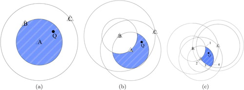
Suppose that the anchor nodes (denoted as A, B, and C) are the neighbour nodes of the target node (denoted as Q). The feedback timing of nodes A, B, and C are assumed to be as QBC, AQC and QAB. Figure 1 shows the sampling region of the target node determined by different number of the anchor nodes. In Figure 1(a), node Q is in the circle with node A as the centre and the distance between the nodes A and B as the radius. In Figure 1(b), the sampling region of node Q, predicted by nodes A and B, is the shadow region. And, in Figure 1(c), with the feedback timing of the three anchor nodes, the initial sampling region of the target node in TSMCL-BPSO algorithm is determined, i.e. the shadow region.

Figure 1. Initial sampling region determined by three anchor nodes.

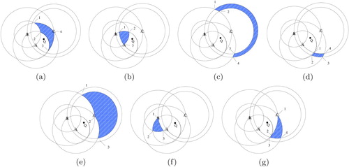
According to the topology relation between the target node and three anchor nodes, there are eight possible sampling regions, illustrated in Figures 1(c) and 2(a–g).

Figure 2. Possible sampling region for different topology.

2.2. MCL sampling region

The final sampling region of TSMCL-BPSO algorithm is formed by overlapping the initial sampling region with MCL sampling region. In the MCL algorithm, each particle is given a certain weight, and the particle set is used to represent the posterior distribution of the possible location of the target node at the next moment. Its emphasis is not on the measuring relative distance between the target node and the anchor nodes, but reducing the possible region of the target node [17, 18]. The MCL algorithm includes node initialization, prediction and filtering. The sampling region of the target node is determined in the prediction phase.

Initialization: Assume that time is split into equal length segments, and $t=\{1,2,3,\dots \}$ is represented as discrete time. At first, there is no any information about the location of the target node, and N sample points are selected randomly in the given region to construct the sample set $L_0=\{l_0^0,l_0^1,\dots ,l_0^{N-1}\}$.

Prediction: Let $V_{max}$ be the maximum moving speed of the target node, and $d(l_t|l_{t-1})$ is the Euclidean distance of the target node at moments T and T−1. If the moving speed of the target node is uniformly distributed, the probability density function (PDF) of the node location also obeys uniformly distributed, expressed by [19] (2) $p(l_t|l_{t-1})=\{\begin{array}{ll}1/\pi V_{max}^2& \mathrm{if}d(l_t|l_{t-1})<V_{max},\\ 0& \mathrm{if}d(l_t|l_{t-1})\ge V_{max}.\end{array}$(2)

The sampling region is a shadow region, shown in Figure 3(a).

Figure 3. Sampling region of MCL.

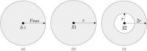
Filtering: The target node filters the sampling points according to the observed information of one-hop and two-hop anchor nodes of the target node. Assume $S1$ is the one-hop anchor node set, $S2$ is the two-hop anchor node set, l is the sampling particle, and s represents the anchor node. Then, the filter condition of sampling point l can be written as (3) $\begin{array}{rl}\mathrm{filter}(l_t^i)& =[\mathrm{\forall }s\in S1,d(l_t^i,s)\le r]\\ & \cap [\mathrm{\forall }s\in S2,r<d(l_t^i,s)\le 2r].\end{array}$(3) The restricted sampling region is a shadow region, shown in Figure 3(b,c).

2.3. Final sampling region

Assume the coordinates of the anchor nodes A, B and C are ($x_{\mathrm{A}}$, $y_{\mathrm{A}}$ ), ($x_{\mathrm{B}}$, $y_{\mathrm{B}}$) and ($x_{\mathrm{C}}$, $y_{\mathrm{C}}$) respectively, and the distances between A and B, A and C, B and C are $r_1$, $r_2$ and $r_3$, respectively. In Figure 1(c), let (X, Y ) be the coordinates of the node in the shadow region, then we have (4) $\begin{array}{rl}(X-x_{\mathrm{A}}{)}^2+(Y-y_{\mathrm{A}}{)}^2& \le r_1^2,\\ r_1^2\le {(X-x_{\mathrm{B}})}^2+{(Y-y_{\mathrm{B}})}^2& \le r_3^2,\\ {(X-x_{\mathrm{C}})}^2+{(Y-y_{\mathrm{C}})}^2& \le r_2^2.\end{array}$(4)

The sampling region is related to the number of rings determined by the feedback timing of the anchor nodes. It is assumed that the number of rings is h, then the number of vertices of the sampling region is written as (5) $3\le k\le h+3,h\in [0,2].$(5)

The intersection of the two circles is at most 2, and only one is the vertices in the shadow region. So, the vertices outside the shadow sampling region need to be eliminated. In Figure 1(c), the coordinates of the vertices 1, 2, 3, and 4 can be expressed as (6) $\begin{array}{rl}& (x_1,y_1):\{\begin{array}{l}{(x_1-x_{\mathrm{A}})}^2+{(y_1-y_{\mathrm{A}})}^2=r_1^2,\\ {(x_1-x_{\mathrm{B}})}^2+{(y_1-y_{\mathrm{B}})}^2=r_1^2,\end{array}\end{array}$(6) (7) $\begin{array}{rl}& (x_2,y_2):\{\begin{array}{l}{(x_2-x_{\mathrm{B}})}^2+{(y_2-y_{\mathrm{B}})}^2=r_1^2,\\ {(x_1-x_{\mathrm{C}})}^2+{(y_2-y_{\mathrm{C}})}^2=r_2^2,\end{array}\end{array}$(7) (8) $\begin{array}{rl}& (x_3,y_3):\{\begin{array}{l}{(x_3-x_{\mathrm{B}})}^2+{(y_3-y_{\mathrm{B}})}^2=r_3^2,\\ {(x_3-x_{\mathrm{C}})}^2+{(y_3-y_{\mathrm{C}})}^2=r_2^2,\end{array}\end{array}$(8) (9) $\begin{array}{rl}& (x_4,y_4):\{\begin{array}{l}{(x_4-x_{\mathrm{A}})}^2+{(y_4-y_{\mathrm{A}})}^2=r_1^2,\\ {(x_4-x_{\mathrm{B}})}^2+{(y_4-y_{\mathrm{B}})}^2=r_3^2.\end{array}\end{array}$(9) According to the constraint equation (4(4) $\begin{array}{rl}(X-x_{\mathrm{A}}{)}^2+(Y-y_{\mathrm{A}}{)}^2& \le r_1^2,\\ r_1^2\le {(X-x_{\mathrm{B}})}^2+{(Y-y_{\mathrm{B}})}^2& \le r_3^2,\\ {(X-x_{\mathrm{C}})}^2+{(Y-y_{\mathrm{C}})}^2& \le r_2^2.\end{array}$(4) ), the intersection points outside the sampling region are filtered out. In Figure 4(a), there are three lines in (or tangent to) the shadow sampling region, which can be represented as (10) $\begin{array}{rl}{l}_1:x& =x_{\mathrm{B}}+r_1,\\ l_2:x& =x_{\mathrm{A}}+r_1,\\ l_3:y& =y_{\mathrm{B}}-r_1.\end{array}$(10) The shadow sampling region determined by the feedback timing of the anchor nodes is irregular. For convenience, its enclosing rectangular is regarded as the initial sampling region of the target node, denoted as $R_1$. Then, the coordinates of vertices E and F of the enclosing rectangular are obtained by (11) $\begin{array}{rl}E(x_E,y_E)& :\{\begin{array}{l}{x}_E=min\{min\left(x_i\right),\\ x_{\mathrm{B}}+r_1,x{}_{\mathrm{A}}+r_1\},\\ y_E=min\{min\left(y_i\right),\\ y{}_{\mathrm{B}}-r_1\},\end{array}i=1,2,\dots 4,\end{array}$(11) (12) $\begin{array}{rl}F(x_F,y_F)& :\{\begin{array}{l}{x}_F=max\{max\left(xi\right),\\ x{}_{\mathrm{B}}+r_1,x_{\mathrm{A}}+r_1\},\\ y_F=max\{max\left(yi\right),\\ y{}_{\mathrm{B}}-r_1\},\end{array}i=1,2,\dots 4.\end{array}$(12)

Figure 4. Sampling region of TSMCL-BPSO.

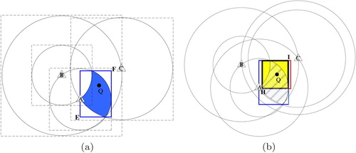
In the MCL algorithm, the sampling region of the target node is a circle. Similarly, the circumscribing square of the sampling circle is regarded as the possible MCL sampling region $R_2$. Therefore, the overlap of $R_1$ and $R_2$ is the final sampling region R of the target node, i.e. the rectangle with H and I as its vertex in Figure 4(b). The coordinates of vertices H and I of this are written as (13) $\begin{array}{rl}H(x_H,y_H)& :\{\begin{array}{l}{x}_H=max\left\{x_E,X_{t-1}-V_{max}\right\},\\ y_H=max\left\{y_E,Y_{t-1}-V_{max}\right\},\end{array}\end{array}$(13) (14) $\begin{array}{rl}I(x_I,y_I)& :\{\begin{array}{l}{x}_I=min\left\{x_E,X_{t-1}+V_{max}\right\},\\ y_I=min\left\{y_E,Y_{t-1}+V_{max}\right\}.\end{array}\end{array}$(14)

3. Particle optimization and node localization

After the final sampling region is determined, the target localization is implemented. In the localization, the target node is represented by particles, and the real location of the target node can be searched by PSO strategy.

3.1. Principle of PSO strategy

The PSO algorithm is an intelligent optimization method to simulate the predatory behaviour of birds [20]. It can be widely used in many engineering fields, such as target tracking, navigation guidance, state monitoring, fault detection, parameter estimation and system identification, etc. [21]. In PSO strategy, a group of particles are initialized. The fitness of particle is determined by objective function, and the particle moves in sampling region at a certain speed and direction. Particles swarm follows the current optimal particle and search in the solution space. The particle dynamically adjusts its position and speed according to the optimal solution searched by itself and particle swarm. Suppose that there are M particles in D-dimensional searching region. Let $x_{id}=(x_{i1},x_{i2},\dots ,x_{id},i=1,2,\dots ,M)$ indicate the position of ith particle, and $v_{id}=(v_{i1},v_{i2},\dots ,v_{id})$ indicate the velocity of the ith particle. The individual optimum position of ith particle is $p_{id}=(p_{i1},p_{i2},\dots ,p_{id})$, and the global optimum position of particle swarm is $p_{gd}=(p_{g1},p_{g2},\dots ,p_{gd})$. Then the evolution equations of the ith particle's speed and position are [22] (15) $\begin{array}{rl}{v}_{id}^{k+1}& =w{v}_{id}^k+c_1{r}_1\left(p_{id}^k-x_{id}^k\right)+c_2{r}_2\left(p_{gd}^k-x_{id}^k\right),\end{array}$(15) (16) $\begin{array}{rl}{x}_{id}^{k+1}& =x_{id}^k+v_{id}^k,\end{array}$(16) where w is inertia weighting factor, $v_{id}^k$ is the speed of ith particle after k iterations, $c_1$ and $c_2$ are cognitive learning factors and social learning factors, respectively, $r_1$ and $r_2$ are independent random numbers, $p_{id}^k$ and $p_{gd}^k$ are the individual optimum and global optimum for k iterations, and $x_{id}^k$ is the position of ith particle after k iterations.

3.2. Improved PSO strategy

The PSO strategy has the advantage of less parameter setting, but the particle is prone to blind phenomenon in global optimization, easily resulting in premature convergence and falling into the local optimum. In order to solve the problem, in the initial searching stage, particle swarm search in sampling region at a higher moving speed (step size), so as to speed up searching process. As the number of iterations increases, particle swarm will gradually approach the global optimum, at which time the step size is reduced to enhance the local searching ability of individual particle. On the other hand, PSO strategy has the disadvantage of weight degradation, and which can be solved by the resampling method [23]. However, resampling only copies the samples with higher weight, which can lead to particle impoverishment [24]. Therefore, distributed estimation and particle replication are taken to improve particle impoverishment, increase population diversity, and achieve population evolution.

Firstly, the initial step size in particle optimization is set up, which is usually given according to the empirical value. The moving step of particle is adjusted adaptively according to the initial step size and the number of iterations, which is written as (17) $v_{id}^k=v_{id}^0\cdot e^{((ite{r}_{max}-k)/ite{r}_{max})},$(17) where $ite{r}_{max}$ is the maximum number of iterations. Substituted Equation (17(17) $v_{id}^k=v_{id}^0\cdot e^{((ite{r}_{max}-k)/ite{r}_{max})},$(17) ) into Equations (15(15) $\begin{array}{rl}{v}_{id}^{k+1}& =w{v}_{id}^k+c_1{r}_1\left(p_{id}^k-x_{id}^k\right)+c_2{r}_2\left(p_{gd}^k-x_{id}^k\right),\end{array}$(15) ) and (16(16) $\begin{array}{rl}{x}_{id}^{k+1}& =x_{id}^k+v_{id}^k,\end{array}$(16) ), and the updated particle velocity and position are expressed, respectively, by (18) $\begin{array}{rl}{v}_{id}^{k+1}& =w{v}_{id}^0\cdot e^{((ite{r}_{max}-k)/ite{r}_{max})}+c_1{r}_1\left(p_{id}^k-x_{id}^k\right)\\ & +c_2{r}_2\left(p_{gd}^k-x_{id}^k\right),\end{array}$(18) (19) $\begin{array}{rl}{x}_{id}^{k+1}& =x_{id}^k+v_{id}^0\cdot e^{((ite{r}_{max}-k)/ite{r}_{max})}.\end{array}$(19) Particle replication is designed to increase particle diversity while avoiding the introduction of particles with poor fitness into the next generation. The distributed estimation is a random searching method based on the probability distribution of variables [25], which can realize the individual evolution. By sampling and spatial distribution of excellent individuals, a probabilistic distribution model is constructed to form the next generation of individuals. Assuming that the optimization variables are independent and obey the Gauss distribution, particle replication is performed by the following Equations (20(20) $\begin{array}{rl}{x}_{\mu ,\sigma }& =r_{norm}\cdot \sigma +\mu ,\end{array}$(20) ) and (21(21) $\begin{array}{rl}{r}_{norm}& =\sqrt{-2\ln r_1}\cdot \sin \left(2\pi r_2\right),\end{array}$(21) ), to obtain the dominant population: (20) $\begin{array}{rl}{x}_{\mu ,\sigma }& =r_{norm}\cdot \sigma +\mu ,\end{array}$(20) (21) $\begin{array}{rl}{r}_{norm}& =\sqrt{-2\ln r_1}\cdot \sin \left(2\pi r_2\right),\end{array}$(21) where $r_1$ and $r_2$ are the random numbers of [0, 1], and σ and μ are the mean value and standard deviation of particles.

Let $d_j$ represent the distance between the real coordinate of the target node and jth anchor node. The coordinate of ith particle is ($x_{id}$, $y_{id}$), and the coordinate of the anchor node is ($x_j$, $y_j$), $j=1,2,\dots ,S$. Theoretically, the closer anchor node is to the actual location of the target node, the more influence it will have on positioning accuracy of the target node. The inertia weight factor is defined as (22) $w_j=\sum _{j=1}^S{d}_j/d_j(j=1,2,\dots S).$(22) In our algorithm, the particle with minimum fitness function is the optimum particle. Then, the fitness function of the particle is defined as (23) $fid=\frac{1}{S}\sum _{j=1}^S(1/w_j)\cdot \left|\sqrt{{\left(x_{id}-x_j\right)}^2+{\left(y_{id}-y_j\right)}^2}-d_j\right|.$(23)

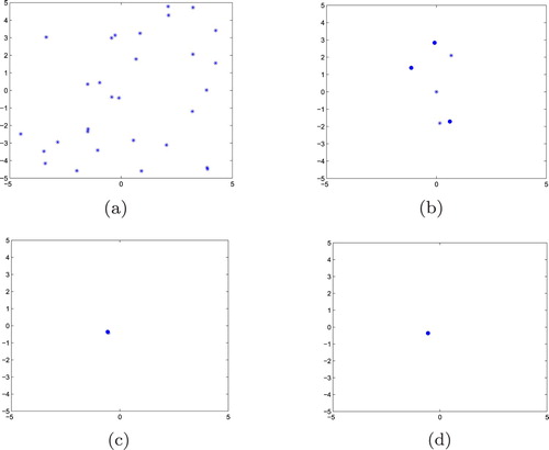
The global optimization ability comparison between TSMCL-BPSO and PSO strategy is shown in Figures 5 and 6. In simulations, the initial position of anchor nodes and target nodes in the monitoring area is generated randomly, and the movement of target nodes is also random. Therefore, the sampling region in TSMCL-BPSO algorithm is different in each simulation. Assume that the final sampling region R of the target node is a rectangle with a side length of 10 m. In region R, 30 particles are randomly thrown, and the PSO and TSMCL-BPSO algorithms are executed to search the global optimum location of target nodes, respectively. From Figures 5 and 6, we can see that compared with the PSO algorithm, the particle in TSMCL-BPSO algorithm can search the global optimum position of target node in a relatively short time.

Figure 5. Particle optimization process in PSO algorithm.

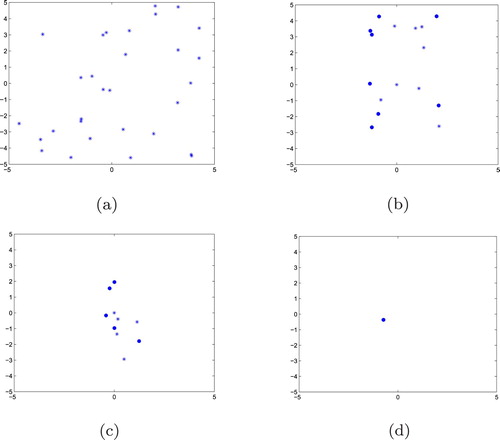
Figure 6. Particle optimization process in TSMCL-BPSO algorithm.

3.3. Target node localization

In the proposed TSMCL-BPSO algorithm, the node localization procedure is shown in Figure 7.

Figure 7. Node location procedure.

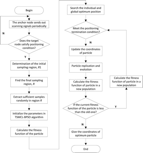
1. The anchor node sends out scanning signals to the neighbours periodically.

2. Determine whether the target node meets the positioning condition. (Does the target node receive at least 3 anchor node information?) If the condition is satisfied, turn to Step3, otherwise return to Step1.

3. According to the feedback signal received by the anchor nodes, determine the initial sampling region of the target node, denoted as $R_1$.

4. Let the MCL sampling region, $R_2$, overlap with $R_1$ to find the final sampling region of the target node, R.

5. Exact sufficient samples (particles) in region R.

6. Initialize the parameters in TSMCL-BPSO algorithm, including the population size, initial position, initial velocity and fixed step size of the particle.

7. Calculate the fitness function of particle by Equation (23(23) $fid=\frac{1}{S}\sum _{j=1}^S(1/w_j)\cdot \left|\sqrt{{\left(x_{id}-x_j\right)}^2+{\left(y_{id}-y_j\right)}^2}-d_j\right|.$(23) ).

8. According to the fitness function of particle, search the individual and global optimum position.

9. Judge whether particle meets the positioning termination condition. (The particle fitness is within a given range, or the number of iterations reaches the maximum number.) If the condition is satisfied, turn to Step14, otherwise continue with Step10.

10. Update the coordinate of the particle by Equations (18(18) $\begin{array}{rl}{v}_{id}^{k+1}& =w{v}_{id}^0\cdot e^{((ite{r}_{max}-k)/ite{r}_{max})}+c_1{r}_1\left(p_{id}^k-x_{id}^k\right)\\ & +c_2{r}_2\left(p_{gd}^k-x_{id}^k\right),\end{array}$(18) ) and (19(19) $\begin{array}{rl}{x}_{id}^{k+1}& =x_{id}^k+v_{id}^0\cdot e^{((ite{r}_{max}-k)/ite{r}_{max})}.\end{array}$(19) ).

11. Particle replication and new population forming by Equations (20(20) $\begin{array}{rl}{x}_{\mu ,\sigma }& =r_{norm}\cdot \sigma +\mu ,\end{array}$(20) ) and (21(21) $\begin{array}{rl}{r}_{norm}& =\sqrt{-2\ln r_1}\cdot \sin \left(2\pi r_2\right),\end{array}$(21) ).

12. Calculate the fitness function of the particle in a new population.

13. If the current fitness function of the particle is less than the fitness function it has experienced, then the historical optimum position is replaced by the current position. Then, return to Step9.

14. Give the coordinates of optimum particle and terminate the localization procedure of the target node.

4. Experiment results

Experiments are performed with Intel (R), Core (TM), i5-2450MCPU, clocked 2.50 GHz, 4 GB memory platforms, and Matlab7.0 simulation environment. In the experiment, the anchor nodes are randomly deployed in a barrier-free monitoring area. It is assumed that each anchor node has the capability of measuring and judging whether other nodes are within its communication range. The movement of the target node is based on random waypoint model [26], and independent of each other. The simulation parameters and its values are shown in Table 1 [27–29].

Table 1. Clustering evaluate matrix.

Parameters	Values
Monitoring area	$200\mathrm{m}\cdot 200\mathrm{m}$
Number of anchor nodes	80
Number of target nodes	20
Node communication radius	50 m
Node moving speed	[0, 70 m/s]
Population size	30
Maximum number of iterations	100
Number of experiments	50
Population size	30
Search dimensions	2
Cognitive learning factors	1.2
Social learning factors	0.5
Initial step size	50
Number of replication	4

4.1. Outlier eliminating and positioning error

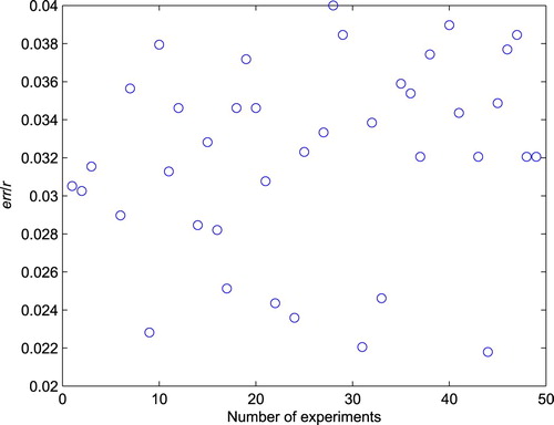
According to the fitness function, the position difference between the particle and the target node can be calculated. The smaller the particle's fitness is, the closer the particle is to the real coordinate of target node. The localization performance is usually evaluated by positioning error, which is defined as (24) $err=\sum _{i=1}^P\sqrt{{\left(x_i-X_i\right)}^2+{(y_i-Y_i)}^2}/rP,$(24) where ($x_i$, $y_i$) and ($X_i$, $Y_i$) are the estimated coordinate and real coordinate of target node, respectively, r is the communication radius of WSN node, and P is the number of experiments.

Gross errors may occur in each experiment. For example, external shocks, mechanical shocks, and electromagnetic interference, etc., can result in the changing position of the target node. The outliers (the points that reach gross error) greatly affect positioning accuracy. The error in range of gross error is an effective error, and the error produced by outlier is an invalid error. Outlier eliminating is necessary in localization algorithm. The common criterion for error analysis includes $3\sigma$, Grubbs and Dixon criterion, etc. The $3\sigma$ criterion is suitable for the number of experiments more than 30. The Grubbs criterion is generally applicable for the fewer number of experiments. The Dixon criterion is complex, and the results need to be sorted. In the simulations, the $3\sigma$ criterion is used to eliminating outliers. It is assumed that ξ is the coordinates of optimum particle for an experiment, and the mean and variance of ξ can be expressed, respectively, by (25) $\begin{array}{rl}\overline{\xi }& =\sum _{i=1}^P{\xi }_i/P,\end{array}$(25) (26) $\begin{array}{rl}\sigma & =\sqrt{\sum _{i=1}^P{\left({\xi }_i-\overline{\xi }\right)}^2/\left(P-1\right)}.\end{array}$(26)

If the condition $|{\xi }_i-\overline{\xi }|>3\sigma$ is satisfied, it shows that ξ is an outlier and should be eliminated.

The initial distribution of the anchor node and the target node in the monitoring area is shown in Figure 8. Figure 9 depicts the variation of particle fitness with the number of iterations in an experiment. The positioning error of TSMCL-BPSO algorithm is plotted in Figure 10.

Figure 8. Initial nodes distribution.

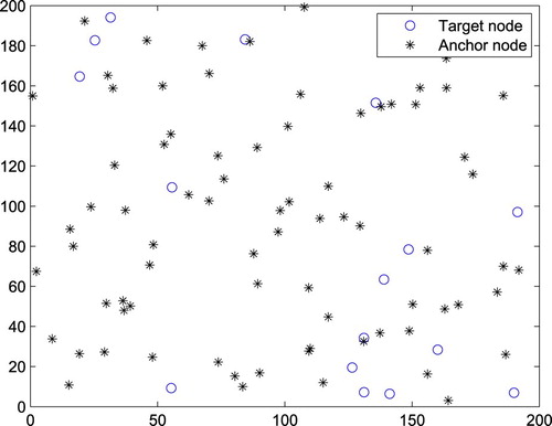
Figure 9. The value of fitness function in an experiment.

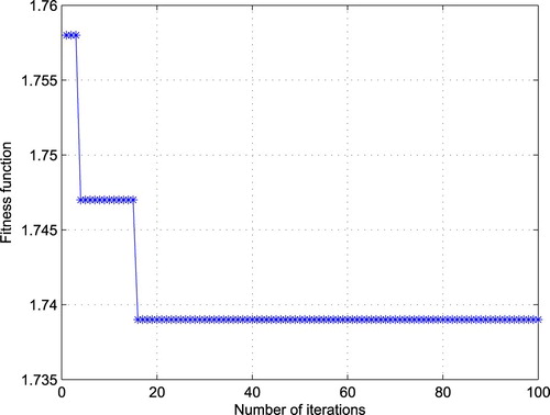
Figure 10. Positioning error in TSMCL-BPSO algorithm.

4.2. Comparison of global optimization ability

In simulations, the initial position of the anchor nodes and the target nodes in the monitoring area is generated randomly, and the movement of the target nodes is also random. Therefore, the sampling region in TSMCL-BPSO algorithm is different in each simulation. Assume that the final sampling region R of the target node is a rectangle with a side length of 10 m. In region R, 30 particles are randomly thrown, and the PSO and TSMCL-BPSO algorithms are executed to search the global optimum location of the target nodes, respectively, illustrated in Figures 9 and 10. It is shown that, compared with the PSO algorithm, the particle in TSMCL-BPSO algorithm can search the global optimum position of the target node in a relatively short time.

4.3. Comparison of positioning error and convergence

Assume that the anchor node density represents the average number of anchor nodes in range of 1 hop of the target node in the monitoring area [30]. The relationship between the anchor node density and positioning error is shown in Figure 11. It is obvious that with the increase of the anchor node density, positioning error is reduced. The reason is that the greater anchor node density is, the more observations node receives, and the higher positioning accuracy is obtained. Also, we can see that TSMCL-BPSO algorithm has the least positioning error.

Figure 11. Relationship between anchor node density and positioning error.

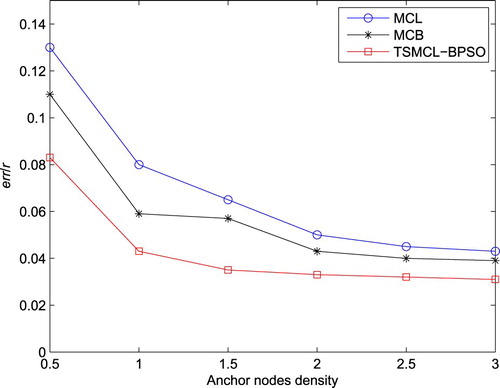
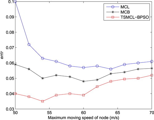
Figure 12 shows the relationship between the maximum moving speed of node $V_{max}$ and positioning error. It can be seen that with the increasing $V_{max}$, positioning error in three algorithms gradually narrowed.

Figure 12. Relationship between maximum moving speed of node and positioning error.

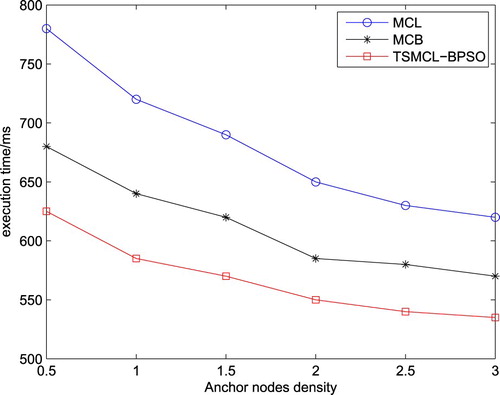
The relationship between the anchor node density and algorithm execution time is shown in Figure 13. The higher the anchor nodes density is, the more observation information the nodes receive, and the shorter searching time for the target node. Compared with MCL and MCB algorithms, the proposed TSMCL-BPSO algorithm reduces the sampling area, which shortens the particle searching time for the target node.

Figure 13. Relationship between the anchor node density and the execution time.

5. Conclusion

In this paper, a time sequence Monte Carlo node localization algorithm based on particle swarm optimization (TSMCL-BPSO) is proposed. The sampling region of the target node is constructed according to the feedback sequence of neighbour anchor nodes of the target node, which reduces the sampling region and filtering time. Experiment results show that the particle fitness and the searching efficiency are improved by adjusting the particle searching step, particle replication and eliminating outliers. Besides, TSMCL-BPSO algorithm has the lower positioning error for different anchor node density and higher node moving speed. For future research, we are currently extending this work to the theoretical analysis of three-dimensional scenes. In addition, the movement of the target node is based on the random waypoint model in this paper. In practical applications, the motion of node follows a certain trajectory. Therefore, the specific node motion model can be introduced to improve the performance of localization algorithm.

Disclosure statement

No potential conflict of interest was reported by the authors.

Additional information

Funding

This work was partially supported by the National Natural Science Foundation of China (61661025, 61661026), and Foundation of A hundred Youth Talents Training Program of Lanzhou Jiaotong University (152022).

References

- HY Shi, WL Wang, NM Kwok, et al. Game theory for wireless sensor networks: a survey. Sensors. 2012;12(7):9055–9097. doi: 10.3390/s120709055
- Rabacy JM, Ammer MJ, da Silva JL, et al. PicoRodio supports ad hoc ultra-low power wireless networking. Computer. 2000;33(7):42–48. doi: 10.1109/2.869369
- Hu L, Evans D. Localization for mobile sensor networks. Proceedings of ACM MobiCom; 2004 Aug; Philadelphia, PA, USA; 2004. p. 45–57.
- Baggio A, Langendoen K. Monte Carlo localization for mobile wireless sensor networks. Proceedings of International Conference on Mobile Ad-Hoc and Sensor Networks; 2006 Dec; Hong Kong, China; 2006. p. 317–328.
- Rudafshani M, Datta S. Localization in wireless sensor networks. Proceedings of ACM International Conference on Information Processing in Sensor Networks; 2007 Apr; Cambridge, MA, USA; 2007. p. 51–60.
- Wang WD, Zhu QX. Rss-based Monte Carlo localisation for mobile sensor networks. IET Commun. 2008;2(5):673–681. doi: 10.1049/iet-com:20070221
- Martins M, Chen H, Sezaki K, et al. Orientation tracking-based Monte Carlo localization for mobile sensor network. Proceedings of IEEE International Conference on Networked Sensing Systems; 2009 Jun; Cambridge, MA, USA; 2009. p. 151–158.
- Rudafshani M, Datta S. Localization in wireless sensor networks. J Chin Comput Syst. 2007;17(5):216–221.
- Yi J, Yang S, Cha H. Multi-hop-based Monte Carlo localization for mobile sensor networks. Proceedings of IEEE Communications Society Conference on Sensor, Mesh and Ad Hoc Communications and Networks; 2007 Oct; Cambridge, MA, USA; 2007. p. 162–171.
- Dong Q, Yu L, Chen Y, et al. Iterative Monte Carlo localization for mobile wireless sensor networks. Chin J Sens Actuat. 2010;23(12):1803–1809.
- Liu Z, Li G, Liu X. Monte-Carlo mobile node localization algorithms based on least squares method. Chin J Sens Actuat. 2012;25(4):541–544.
- Wang PD, Qi CL. An improved node localisation algorithm. Comput Appl Software. 2012;29(8):242–244.
- Li JP, Shi M, Xie Y. A MCL mobile node localisation algorithm based on fuzzy theory. Comput Appl Software. 2013;30(12):147–150.
- Min HQ, Chen H, Luo RH. Active particle in MCL: an evolutionary view. Proceedings of International Conference on Information and Automation; 2009 June; Zhuhai/Macau, China; 2009.
- Chien CH, Wang WY, Hsu CC. Multi-objective evolutionary approach to prevent premature convergence in Monte Carlo localization. Appl Soft Comput. 2017;50:260–279. doi: 10.1016/j.asoc.2016.11.020
- Tian H, Li C, Xie Y, et al. Node localization algorithm for WSN based on time sequence Monte Carlo. Chin J Sens Actuat. 2016;29(11):1724–1730.
- Li G, Chen JJ. A Monte Carlo localization algorithm based on motion prediction. Meas Control Technol. 2013;32(9):100–103.
- Zhao ZJ, Peng Z, Zheng SL. Cognitive radio spectrum assignment based on quantum genetic algorithm. Acta Phys Sin. 2009;58(2):1358–1363.
- Li J, Shi M, Zhong X. Self-adaptive Monte Carlo localization algorithm of mobile nodes in WSN. J Jilin Univ. 2014;44(4):1191–1196.
- Kennedy J, Eberhart R. Particle swarm optimization. Proceedings of IEEE International Conference on Neural Networks; 2002 Dec; Perth, WA, Australia; 2002. p. 1942–1948.
- Kulkarni RV, Venayagamoorthy GK. Particle swarm optimization in wireless-sensor networks: a brief survey. IEEE Trans Syst Man Cybern Part C. 2011;41(2):262–267. doi: 10.1109/TSMCC.2010.2054080
- Cong C. A coverage algorithm for WSN based on the improved PSO. Proceedings of IEEE International Conference on Intelligent Transportation, Big Data and Smart City; 2015 Dec; Halong Bay, Vietnam; 2015. p. 12–15.
- Feng L, Li X, Jiang T, et al. A combined prediction method for the life of product based on PSO with immunity algorithms. Proceedings of IEEE Reliability and Maintainability Symposium; 2014 Jan; Colorado Springs, CO, USA; 2014. p. 1–6.
- Fu X, Jia Y. An improvement on resampling algorithm of particle filters. IEEE Trans Signal Process. 2010;58(10):5414–5420. doi: 10.1109/TSP.2010.2053031
- Wang SY, Wang L, Fang C, et al. Advances in estimation of distribution algorithms. Control Decis. 2012;27(7):961–966.
- Yuan B, Bao Z. Algorithmic research and realization of GPS/COMPASS combined relative positioning. Proceedings of China Satellite Navigation Conference; 2012 Apr; PanYu District, Guangzhou City, China; 2012. p. 447–455.
- Liu XL, Li RJ, Yang P. A bacterial foraging global optimization algorithm based on the particle swarm optimization. Proceedings of IEEE International Conference on Intelligent Computing and Intelligent Systems; 2010 Dec; Xiamen, China; 2010. p. 22–27.
- Mai XF, Li L. An enhanced bacterial foraging optimization with adaptive elimination-dispersal probability and PSO strategy. Proceedings of IEEE International Conference on Natural Computation, Fuzzy Systems and Knowledge Discovery; 2016 Aug; Changsha, China; 2016. p. 161–166.
- Qu BY, Liu DM, Qiao BH. Research on improved particle swarm optimization algorithm. Autom Appl. 2016;2016(11):49–51.
- Sheu JP, Hu WK, Lin JC. Distributed localization scheme for mobile sensor networks. IEEE Trans Mob Comput. 2010;9(4):516–526. doi: 10.1109/TMC.2009.149