Identification of a nonlinear rational model based on bias compensated multi-innovation stochastic gradient algorithm

Abstract

The nonlinear rational model is a generalized nonlinear model and has been gradually applied in modelling many dynamic processes. The parameter identification of a class of nonlinear rational models is studied in this paper. This identification problem is very challenging because of the complexity of the rational model and the coupling between model inputs and outputs. To identify the nonlinear model, a bias compensated multi-innovation stochastic gradient algorithm is presented. The multi-innovation technique replacing the scalar innovation with an information vector is adopted to accelerate the traditional stochastic gradient algorithm. However, the estimate obtained by the accelerated algorithm is biased because of the correlation between the information vector and the noise. To overcome this difficulty, a bias compensation strategy is used. The bias is calculated and compensated to get an unbiased estimate. Theoretical analysis shows that the proposed algorithm can give biased estimates with linear complexity. The proposed algorithm is validated by a numerical experiment and the modelling of the propylene catalytic oxidation.

KEYWORDS:

• Nonlinear rational model
• parameter estimation
• adaptive modelling
• bias compensation
• stochastic gradient algorithm

1. Introduction

To describe the dynamic characteristics of the nonlinear systems, many nonlinear structures have been developed, such as the NARMAX model, Volterra series model, block-oriented nonlinear model and so on [1–4]. In recent years, a model named nonlinear rational model (NRM) has been gradually applied in the modelling and control of nonlinear systems, particularly in some chemical processes and mechanistic systems [5–8]. The NRM is a kind of generalized nonlinear model. Traditional rational model, NARMAX model, integral model, output affine model and linear difference equation model can be seen as its special form [9].

The NRM is defined as the ratio of two polynomial expansions of past inputs, outputs and prediction errors [10]. The identification of the NRM is quite difficult because the NRM cannot be parameterized into a linear-in-parameter system [9–11] and the coupling between model input and output. Despite the difficulties, researchers have reported some results [7,9,12]. For example, to identify the parameters of the NRM, a prediction error algorithm and a new rational model estimation (RME) algorithm were proposed [11,13]. To decrease the computational cost of the above two algorithms, a recursive RME algorithm, an error back propagation algorithm, an implicit least-squares iterative algorithm, two maximum likelihood algorithms and a globally convergent algorithm were derived [5,7,10,14,15]. To determine the NRM’s structure, an orthogonal RME algorithm and a genetic algorithm were investigated [9,11]. Zhu et al. summarized the advances in NRM identification and control [8].

Although these algorithms work well for many NRMs, they have at least O(n²) complexity, which makes them unsuitable for online applications. To decrease the complexity, the stochastic gradient (SG) algorithm is an alternative because it costs only O(n) flops each iteration [16]. There are many gradient-based algorithms, among which, a key term separation gradient iterative algorithm was derived to identify a fractional-order nonlinear system [17], a three-stage forgetting factor SG method was proposed for a Hammerstein system [18] and an auxiliary model stochastic gradient method was studied for a Wiener–Hammerstein system [19].

However, the estimate for the NRM given by the traditional SG algorithm is biased because the information vector is correlated to the noise [10,20,21]. To get unbiased estimates, the bias compensation (BC) technique and instrumental variable (IV) technique are often used, for example, a BC-based method was proposed to estimate the state of charge for lithium-ion batteries [22], a BC-based sign algorithm was addressed to estimate the weight vector of an unknown system [23], an IV method was implemented for detecting and correcting parameter bias within structural equation models [24], a unified model-implied IV approach was reported for structural equation modelling with mixed variables [25]. Sometimes, for the IV method, although there are some guiding principles, it is still very difficult to select an appropriate instrumental variable. Therefore, the BC method is adopted to obtain an unbiased estimate for the NRM in this paper [10].

This paper considers the parameter identification of the so-called ARX-NRM. This NRM contains a process model with nonlinear rational form and its noise model has the same denominator as the process model. This paper investigates this parameter identification in the time domain, without considering modelling error, time-delay estimation, uncertainties in the real systems and frequency-domain identification [26–29]. Meanwhile, this paper discusses the integer adaptive methods for the nonlinear models. Recently, the fractional adaptive method has been an important part of adaptive algorithms. For details, please see [30–33].

The main contributions of this paper are as follows:

1. The parameter identification of an ARX-type nonlinear rational model is considered, which is quite difficult because this model is a nonlinear-in-parameter system and its output is coupled with the input.

2. To accelerate the stochastic gradient algorithm, the multi-innovation technique is integrated into the algorithm, in which the scalar innovation is replaced by the innovation vector.

3. The bias of the multi-innovation stochastic gradient algorithm is calculated by the observations and the previous estimates, and then compensated to get an unbiased estimate.

4. The proposed algorithm is validated by numerical examples and case study. Results indicate that the proposed algorithm can obtain accurate estimates with a fast converge speed.

The rest of this work is organized as follows. In Section 2, the ARX-NRM to be estimated is described. Then an unbiased multi-innovation SG algorithm is presented in Section 3. In the next section, the performance of the proposed algorithm is analysed. Numerical examples and case study are adopted to validate the proposed algorithm in Section 5. Finally, conclusion is summarized in Section 6.

2. Problem description

Consider an ARX-NRM depicted in Figure 1, where $u(k)$, $y(k)$ and $v(k)$ are the input, output and noise, respectively. $f(k)$ and $g(k)$ are two nonlinear polynomials concerning $y(k-i)$ and/or $u(k-j)$, $i,j=1,2,\dots ,r$.

Figure 1. Block diagram of an ARX-NRM.

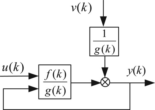
From Figure 1, we can express the output $y(k)$ by (1) $\begin{array}{r}y(k)=\frac{f(k)}{1\text{ + }g(k)}+\frac{1}{1\text{ + }g(k)}v(k),\end{array}$(1) where (2) $\begin{array}{r}\{\begin{array}{l}f(k)=f(y(k-1),\dots ,y(k-r),u(k-1),\dots ,u(k-r)),\\ g(k)=g(y(k-1),\dots ,y(k-r),u(k-1),\dots ,u(k-r)).\end{array}\end{array}$(2)

It can be seen from Figure 1 and Equation (1) that the structure of this NRM is similar to that of the ARX model, $y(k)=\frac{B(z^{-1})}{1+A(z^{-1})}u(k)+\frac{1}{1+A(z^{-1})}v(k)$ [21]. The difference is that the numerator $f(k)$ and denominator $g(k)$ of the NRM are both nonlinear polynomials, and the input $u(k-i)$ is implicit in the nonlinear transfer function. Thus the NRM in Figure 1 is named ARX-NRM.

Multiplying both sides of Equation (1) by $1\text{ + }g(k)$ yields (3) $\begin{array}{r}(1+g(k))y(k)=f(k)+v(k)\end{array}$(3) with (4) $\begin{array}{r}\{\begin{array}{l}f(k)=b_1{\psi }_1(k)+\cdots +b_{n_b}{\psi }_{n_b}(k)\\ g(k)=a_1{\varphi }_1(k)+\cdots +a_{n_a}{\varphi }_{n_a}(k)\end{array}\end{array}$(4) and ${\varphi }_i(k)$, ${\psi }_j(k)$ are scalars with the forms of $u^j(k-i),y^j(k-i)$, $u^m(k-i)y^l(k-j)$, etc. Then we can parameterize the ARX-NRM as follows: (5) $\begin{array}{r}y(k)=-y(k)g(k)+f(k)+v(k)={\mathit{\phi }}^T(k)\mathit{\theta }+v(k),\end{array}$(5) where (6) $\begin{array}{r}\{\begin{array}{l}\mathit{\theta }={[{\mathit{\theta }}_a^T,{\mathit{\theta }}_b^T]}^T\in {\mathbb{R}}^{n\times 1},\\ \mathit{\phi }(k)={[-y(k){\mathit{\phi }}_a^T(k),{\mathit{\phi }}_b^T(k)]}^T\in {\mathbb{R}}^{n\times 1},\\ n=n_a+n_b,\\ {\mathit{\phi }}_a(k)={[{\varphi }_1(k),\dots ,{\varphi }_{n_a}(k)]}^T\in {\mathbb{R}}^{n\times 1},\\ {\mathit{\phi }}_b(k)={[{\psi }_1(k),\dots ,{\psi }_{n_b}(k)]}^T\in {\mathbb{R}}^{n\times 1},\\ {\mathit{\theta }}_a={[a_1,\dots ,a_{n_a}]}^T\in {\mathbb{R}}^{n_a\times 1},\\ {\mathit{\theta }}_b={[b_1,\dots ,b_{n_b}]}^T\in {\mathbb{R}}^{n_b\times 1}.\end{array}\end{array}$(6)

The identification of the ARX-NRM in Figure 1 is transformed into the estimation of the parameter vector $\mathit{\theta }$ based on the observations $\{u(k),y(k){\}}_{k=1}^N$, where $N$ is the data length.

3. Identification algorithm

3.1. Stochastic gradient (SG) algorithm

Consider the parameterized system in Equation (5) and denote the error $e(k)$ as (7) $\begin{array}{r}e(k)=y(k)-{\mathit{\phi }}^T(k)\hat{\mathit{\theta }}(k-1),\end{array}$(7) where $\hat{\mathit{\theta }}(k-1)$ is the parameter estimate at time $k-1$. Sometimes, $e(k)$ is also called innovation [16].

Define a cost function as follows: (8) $\begin{array}{r}V(k)=\frac{1}{2}{e}^2(k).\end{array}$(8) The SG algorithm updates the parameter estimate along the negative gradient direction of the criterion function $V(k)$ until $V(k)$ reaches the minimum. The stochastic gradient of $V(k)$ concerning $\mathit{\theta }$ at time $k$ is (9) $\begin{array}{r}\mathit{g}(k)=-\mathit{\phi }(k)e(k)\text{ = }-\mathit{\phi }(k)(y(k)-{\mathit{\phi }}^T(k)\hat{\mathit{\theta }}(k-1)).\end{array}$(9)

The SG algorithm for identification of $\mathit{\theta }$ is as follows [20]: (10) $\begin{array}{r}\hat{\mathit{\theta }}(k)=\hat{\mathit{\theta }}(k-1)-\eta (k)\mathit{g}(k),\end{array}$(10) where $\eta (k)$ is the variable step size that can be calculated by [16] (11) $\begin{array}{rl}\eta (k)& =\frac{1}{r(k)},r(k)=\lambda r(k-1)+{\mathit{\phi }}^T(k)\mathit{\phi }(k),\\ r(0)& =1,\lambda \in (0,1].\end{array}$(11)

3.2. Multi-Innovation SG (MI-SG) algorithm

Although the SG algorithm costs less calculation than the least-squares algorithm, it converges slowly. To accelerate the algorithm, multi-innovation is introduced [16]. Replacing the single innovation $e(k)$ in Equation (9) with the multi-innovation vector ${\mathit{E}}_p(k)$, and replacing the single information vector $\mathit{\phi }(k)$ with the information matrix ${\mathbf{\Phi }}_p(k)$ gives a stacking gradient ${\mathit{G}}_p(k)$ as follows: (12) $\begin{array}{r}\{\begin{array}{l}{\mathit{G}}_p(k)=-{\mathbf{\Phi }}_p(k){\mathit{E}}_p(k)\in {\mathbb{R}}^{n\times 1},\\ {\mathbf{\Phi }}_p(k)=[\mathit{\phi }(k),\mathit{\phi }(k-1),\dots ,\mathit{\phi }(k-p+1)]\in {\mathbb{R}}^{n\times p},\\ {\mathit{E}}_p(k)={\left[\begin{array}{c}e(k),e(k-1),\dots ,e(k-p+1)\end{array}\right]}^T\in {\mathbb{R}}^{p\times 1},\end{array}\end{array}$(12) where $p$ is the stacking length, ${\mathit{G}}_p(k)$, ${\mathit{E}}_p(k)$ and ${\mathbf{\Phi }}_p(k)$ are the stacked gradient, stacked innovation vector, and stacked information matrix, respectively. Expanding ${\mathit{G}}_p(k)$ yields (13) $\begin{array}{r}{\mathit{G}}_p(k)=-\sum _{i=k-p+1}^k\mathit{\phi }(i)e(i)=-\sum _{i=k-p+1}^k\mathit{g}(i),\end{array}$(13) where $\mathit{g}(i)$ denotes the gradient at time $i$.

It can be seen from Equation (13) that the stacked gradient ${\mathit{G}}_p(k)$ is the sum of recent $p$ gradients, and it can also be regarded as the weighted information vectors, and the weighting coefficient is the innovation at the corresponding time. In short, this summation or weighting increases the size of the gradient, modifies the direction of the gradient and is conducive to accelerating the gradient algorithm. This gradient algorithm using multi-innovation is called multi-innovation SG (MI-SG) algorithm.

Consider Equation (13), the SG estimator Equation (10) is rewritten as (14) $\begin{array}{r}\hat{\mathit{\theta }}(k)=\hat{\mathit{\theta }}(k-1)-\eta (k){\mathit{G}}_p(k).\end{array}$(14) Equations (7)–(14) except Equation (10) construct the MI-SG algorithm.

3.3. Bias compensated MI-SG (BC-MI-SG) algorithm

Let us study the properties of the parameter estimate given by the MI-SG algorithm.

Considering Equations (7) and (9), the stacked gradient ${\mathit{G}}_p(k)$ in Equation (12) is rewritten as (15) $\begin{array}{rl}{\mathit{G}}_p(k)& =-\sum _{i=k-p+1}^k\mathit{\phi }(i)e(i)\\ & =-\sum _{i=k-p+1}^k\mathit{\phi }(i)(y(i)-{\mathit{\phi }}^T(i)\hat{\mathit{\theta }}(i-1))\\ & =-\sum _{i=k-p+1}^k\mathit{\phi }(i)({\mathit{\phi }}^T(i){\mathit{\theta }}_0\\ & +v(i)-{\mathit{\phi }}^T(i)\hat{\mathit{\theta }}(i-1))\\ & =-\sum _{i=k-p+1}^k(\mathit{\phi }(i){\mathit{\phi }}^T(i){\mathit{\theta }}_0+\mathit{\phi }(i)v(i)\\ & -\mathit{\phi }(i){\mathit{\phi }}^T(i)\hat{\mathit{\theta }}(i-1))\\ & =-\sum _{i=k-p+1}^k\mathbf{\Omega }{\mathit{\theta }}_0-\sum _{i=k-p+1}^k\mathit{T}(i)\\ & +\sum _{i=k-p+1}^k\mathbf{\Omega }\hat{\theta }(i-1),\end{array}$(15) where $\mathit{T}(i)=\mathit{\phi }(i)v(i)$, $\mathbf{\Omega }=\mathit{\phi }(i){\mathit{\phi }}^T(i)$ and ${\mathit{\theta }}_0$ denote the true parameter vector.

Considering Equations (15) and (14) becomes (16) $\begin{array}{rl}\hat{\mathit{\theta }}(k)& =\hat{\mathit{\theta }}(k-1)+\eta (k)\sum _{i=k-p+1}^k\mathbf{\Omega }{\mathit{\theta }}_0+\eta (k)\\ & \times \sum _{i=k-p+1}^k\mathit{T}(i)-\eta (k)\sum _{i=k-p+1}^k\mathbf{\Omega }\hat{\mathit{\theta }}(i-1).\end{array}$(16) Taking expectation on both sides of Equation (16) yields (17) $\begin{array}{rl}E\{\hat{\mathit{\theta }}(k)\}& =E\{\hat{\mathit{\theta }}(k-1)\}+\eta (k)\sum _{i=k-p+1}^k\mathbf{\Omega }{\mathit{\theta }}_0\\ & +\eta (k)E\left\{\sum _{i=k-p+1}^k\mathit{T}(i)\right\}\\ & -\eta (k)E\left\{\sum _{i=k-p+1}^k\mathbf{\Omega }\hat{\mathit{\theta }}(i-1)\right\}.\end{array}$(17) Supposing $\mathbf{\Omega }$ is not related to $\hat{\mathit{\theta }}(i-1)$, and using the conditional expectation formula [20] (18) $\begin{array}{r}E\{f(\mathit{x})\mathit{y}\}=E\{E\{f(\mathit{x})|\mathit{y}\}\mathit{y}\},\end{array}$(18) The fourth item on the right side of Equation (17) can be written as (19) $\begin{array}{rl}& -\eta (k)E\left\{\sum _{i=k-p+1}^k\mathbf{\Omega }\hat{\mathit{\theta }}(i-1)\right\}\\ & =-\eta (k)\mathbf{\Omega }E\left\{\sum _{i=k-p+1}^k\hat{\mathit{\theta }}(k-1)\right\}.\end{array}$(19) Equation (17) becomes (20) $\begin{array}{rl}E\{\hat{\mathit{\theta }}(k)\}& =E\{\hat{\mathit{\theta }}(k-1)\}+\eta (k)\mathbf{\Omega }\sum _{i=k-p+1}^k{\mathit{\theta }}_0+\eta (k)\\ & \times \sum _{i=k-p+1}^{k}E\{\mathit{T}(i)\}-\eta (k)\mathbf{\Omega }\\ & \times \sum _{i=k-p+1}^{k}E\{\hat{\mathit{\theta }}(i-1)\}.\end{array}$(20) When $k\to \mathrm{\infty }$, $E\{\hat{\mathit{\theta }}(k)\}=E\{\hat{\mathit{\theta }}(k-1)\}$, we have (21) $\begin{array}{rl}& \underset{k\to \mathrm{\infty }}{lim}\sum _{i=k-p+1}^{k}E\{\hat{\mathit{\theta }}(i-1)-{\mathit{\theta }}_0\}\\ & ={\mathbf{\Omega }}^{-1}\sum _{i=k-p+1}^{k}E\{\mathit{T}(i)\}\ne \mathbf{0}.\end{array}$(21) It can be seen from Equation (21) that the parameter estimate obtained by the MI-SG algorithm is biased. We can find that the bias ${\mathbf{\Omega }}^{-1}\sum _{i=k-p+1}^{k}E\{\mathit{T}(i)\}$ is caused by the $\eta (k)\sum _{i=k-p+1}^k\mathit{T}(i)$ on the right of Equation (16). To obtain an unbiased estimate, this term must be subtracted from the right of Equation (14), i.e. (22) $\begin{array}{r}\hat{\mathit{\theta }}(k)=\hat{\mathit{\theta }}(k-1)-\eta (k){\mathit{G}}_p(k)-\eta (k)\sum _{i=k-p+1}^k\mathit{T}(i).\end{array}$(22) However, $\mathit{T}(i)$ cannot be calculated by $\mathit{\phi }(i)v(i)$ because of the unknown $v(i)$. For the ARX-NRM in Figure 1, considering Equation (6) and replacing the unknown $v(i)$ by $e(i)$, $\mathit{T}(i)$ is calculated by (23) $\begin{array}{rl}\mathit{T}(i)=\mathit{\phi }(i)v(i)& =\left[\begin{array}{c}-y(i)v(i){\mathit{\phi }}_a(i)\\ v(i){\mathit{\phi }}_b(i)\end{array}\right]\\ & =\left[\begin{array}{c}-y(i)v(i){\mathit{\phi }}_a(i)\\ {\mathbf{0}}_{n_b\times 1}\end{array}\right]\\ & \approx \left[\begin{array}{c}-y(i)e(i){\mathit{\phi }}_a(i)\\ {\mathbf{0}}_{n_b\times 1}\end{array}\right]\end{array}$(23) Substituting Equation (23) into Equation (22) yields (24) $\begin{array}{rl}\hat{\mathit{\theta }}(k)& =\hat{\mathit{\theta }}(k-1)-\eta (k){\mathit{G}}_p(k)\text{ + }\eta (k)\\ & \times \sum _{i=k-p+1}^{k}y(i)e(i)\left[\begin{array}{c}{\mathit{\phi }}_a(i)\\ {\mathbf{0}}_{n_b\times 1}\end{array}\right],\end{array}$(24) Equations (7)–(13) and Equation (24) (except Equation (10)) construct the bias compensated MI-SG (BC-MI-SG) algorithm.

4. Performance analysis

4.1. Computational analysis

The calculation costs of each iteration of the SG, MI-SG, RLS and BC-MI-SG algorithms are shown in Table 1. It is seen that:

1. The computational burden of the three SG algorithms is all $O(n)$.

2. The MI-SG and the BC-MI-SG algorithm cost more computations than the SG algorithm because of the multi-innovation.

3. The proposed algorithm costs less computation than the recursive least squares (RLS) algorithm, whose complexity is $O(n^2)$ [9,16].

Table 1. Computational costs of the SG, MI-SG, BC-MI-SG, and RLS algorithms.

	SG	MI-SG	BC-MI-SG	RLS
Computation cost	$6n+2$	$5n+np+2$	$5n+np+n_a+5$	$4n^2+6n$
$n=10,p=3,$
$n_a=5$	62	82	90	460
$n=100,p=3,$
$n_a=50$	602	802	855	40,600

4.2. Convergence analysis

According to Section 3.3, for the proposed BC-MI-SG algorithm, Equation (17) becomes (25) $\begin{array}{rl}E\{\hat{\mathit{\theta }}(k)\}& =E\{\hat{\mathit{\theta }}(k-1)\}+\eta (k)\sum _{i=k-p+1}^k\mathbf{\Omega }{\mathit{\theta }}_0\\ & -\eta (k)E\left\{\sum _{i=k-p+1}^k\mathbf{\Omega }\hat{\mathit{\theta }}(i-1)\right\}.\end{array}$(25) When $k\to \mathrm{\infty }$, $E\{\hat{\mathit{\theta }}(k)\}=E\{\hat{\mathit{\theta }}(k-1)\}$, Equation (25) can be rewritten as (26) $\begin{array}{r}\underset{k\to \mathrm{\infty }}{lim}\sum _{i=k-p+1}^{k}E\{\hat{\mathit{\theta }}(i-1)-{\mathit{\theta }}_0\}=\mathbf{0}.\end{array}$(26) Consider $\underset{k\to \mathrm{\infty }}{lim}E\{\hat{\mathit{\theta }}(k-j)\}=E\{\hat{\mathit{\theta }}(k)\},j=0,1,\cdots ,p-1$, Equation (26) is rewritten as (27) $\begin{array}{r}p\underset{k\to \mathrm{\infty }}{lim}E\{\hat{\mathit{\theta }}(k)-{\mathit{\theta }}_0\}=\mathbf{0},\end{array}$(27) which means $\underset{k\to \mathrm{\infty }}{lim}E\{\hat{\mathit{\theta }}(k)\}={\mathit{\theta }}_0$.

5. Experiment results

5.1. Numerical example

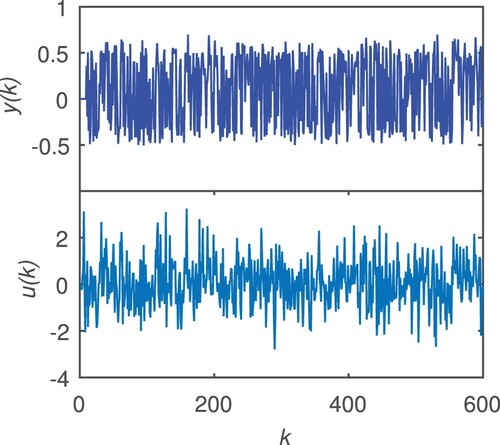
Consider an ARX-NRM in Equation (1) with (28) $\begin{array}{r}\{\begin{array}{l}f(k)=0.5y(k-1)u(k-2)+u(k-1),\\ g(k)=1+u^2(k-1)+y^2(k-1),\end{array}\end{array}$(28) where the input $u(k)$ is a Gaussian signal with mean zero and variance ${1.0}^2$. A noise $v(k)$ with mean zero is added to the model. 600 observations are collected and depicted in Figure 2. The initial value of each entry of the parameter vector is set to $1\times {10}^{-6}$ and the estimation error is defined as $\delta (\mathrm{\%})=\frac{\Vert \hat{\mathit{\theta }}(N)-{\mathit{\theta }}_0\Vert }{\Vert {\mathit{\theta }}_0\Vert }\times 100$.

1. Results using BC-MI-SG, MI-SG, SG and RLS algorithms

Figure 2. Curves of the observed data.

The parameter estimates using the proposed BC-MI-SG are shown in Table 2, and the estimation errors are depicted in Figure 3, where ${\sigma }^2={0.01}^2,\lambda =0.4,p=3$. For comparison, the parameter estimates given by the SG, RLS and MI-SG algorithms are also listed in Table 2, and the estimation errors using the last three algorithms are also depicted in Figure 3.

Figure 3. Estimation errors using the SG, MI-SG and BC-MI-SG algorithms.

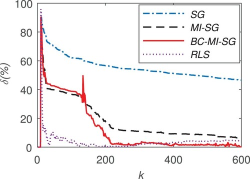
Table 2. Estimates using the SG, MI-SG, RLS and BC-MI-SG algorithms.

Algorithm		50	100	200	400	600	True
SG	$a_1$	0.3565	0.5624	0.7392	0.8683	0.9116	1.0000
	$a_2$	0.0027	0.0085	0.0268	0.0984	0.1741	1.0000
	$b_1$	0.3044	0.3526	0.4077	0.4083	0.4203	0.5000
	$b_2$	0.6456	0.7483	0.8694	0.8782	0.9116	1.0000
	$\delta (\mathrm{\%})$	69.5595	62.2554	56.5903	51.2437	46.5461
MI-SG	$a_1$	0.8569	0.9600	1.1180	0.9686	0.9962	1.0000
	$a_2$	0.3042	0.3439	0.7279	0.8385	0.8885	1.0000
	$b_1$	0.4545	0.4401	0.4617	0.4793	0.4897	0.5000
	$b_2$	0.9159	0.9551	1.1138	0.9904	0.9842	1.0000
	$\delta (\mathrm{\%})$	39.7595	36.6965	17.7479	9.2127	6.2787
RLS	$a_1$	0.9816	0.9803	0.9994	0.9760	0.9802	1.0000
	$a_2$	0.8819	0.9111	0.9975	0.9494	0.9291	1.0000
	$b_1$	0.4808	0.4951	0.5008	0.4907	0.4898	0.5000
	$b_2$	0.9758	0.9799	0.9970	0.9812	0.9842	1.0000
	$\delta (\mathrm{\%})$	6.8482	5.1813	0.2234	3.3156	4.2167
BC-MI-SG	$a_1$	0.8227	0.9661	1.0815	1.0023	1.0045	1.0000
	$a_2$	0.2633	0.3063	0.9366	0.9834	1.0012	1.0000
	$b_1$	0.4503	0.4358	0.4804	0.4912	0.4994	0.5000
	$b_2$	0.8948	0.9599	1.1108	1.0094	1.0007	1.0000
	$\delta (\mathrm{\%})$	42.5233	38.7559	8.4748	1.1752	0.2646

It can be seen that:

1. In Figure 3, all curves decrease when k increases, which means that the estimation errors of the three algorithms become small with the new data being used.

2. The error curves of the two algorithms with MI are almost the same, which are far lower than that of the SG algorithm. In other words, the parameter estimates given by the two MI-SG algorithms are more accurate than those given by the SG algorithm.

3. Among the two curves with MI, the curve of the proposed BC-MI-SG algorithm is at the bottom, which shows that the estimation error given by the proposed algorithm is smaller. That is to say, the bias compensation can improve the estimation accuracy of the MI-SG algorithm.

4. In the second half of identification, the curve of the RLS algorithm has little difference with the proposed algorithm, which implies the RLS algorithm can give an accurate estimate for the ARX-NRM. However, the RLS algorithm costs too much computation to prevent its application in some situations that needs fast identification (see Table 1 for more details).

5. Results using the BC-MI-SG algorithm with different noise variances

To show the performance of the proposed algorithm under different noise levels, we estimate the ARX-NRM in Equation (28) using the BC-MI-SG algorithm with ${\sigma }^2={0.01}^2,{0.02}^2,{0.04}^2$. The estimation errors using different ${\sigma }^2$ are depicted in Figure 4.

Figure 4. Estimation errors using BC-MI-SG with different noise variances.

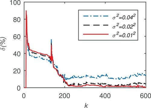
It can be seen that:

1. For a given noise variance ${\sigma }^2$, the overall trend of the estimation error decreases with the increase of $k$.

2. When the variance is small, the curve of the estimation error is relatively smooth. With the increase of variance, the fluctuation of the error curve increases.

3. The estimation error of ${\sigma }^2={0.01}^2$ is smaller than those of the ${\sigma }^2={0.02}^2$ and ${\sigma }^2={0.04}^2$. That is, a larger ${\sigma }^2$ is not conducive to the improvement of the estimate's accuracy.

5.2. Case study

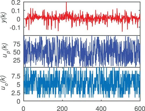
A chemical model describing propylene catalytic oxidation with the following structure [5,15,34] is used to validate the proposed algorithm, $\begin{array}{r}y(k)=\frac{b{C}_p(k)}{1+a\frac{C_p(k)}{C_o^{0.5}(k)}}+\frac{v(k)}{1+a\frac{C_p(k)}{C_o^{0.5}(k)}}\end{array}$where two inputs $C_o(k)$ and $C_p(k)$ are the oxygen and propylene concentrations at time $k$ respectively. The rate of disappearance of propylene $y(k)$ is taken as the output variable. The true values are $a_0=0.231,b_0=7.28\times {10}^{-4}$. The inputs $C_o(k)$ and $C_p(k)$ are taken as random integers between $(1,100)$ and between $(1,10)$ respectively, $\{v(k)\}$ is taken as a white noise sequence with mean zero and variance ${\sigma }^2={0.1}^2$. The curve of 600 observed data is shown in Figure 5.

Figure 5. Curve of the propylene catalytic oxidation data.

Following ARX-NRM structure is used: $\begin{array}{rl}y(k)& =\frac{f(k)}{g(k)}+\frac{1}{g(k)}v(k)\text{with}\\ f(k)& =b{u}_p(k),g(k)=1+a\frac{u_p(k)}{u_o(k)}.\end{array}$Estimate using proposed BC-MI-SG algorithm with $\lambda =0.4,p=3$ is listed in Table 3, where the estimation error is calculated by the following formula: $\delta (N)=\left(\Vert \frac{a_0-\hat{a}(N)}{a_0}\Vert +\Vert \frac{b_0-\hat{b}(N)}{b_0}\Vert \right)\times 100$.

Table 3. Results using the SG, MI-SG and BC-MI-SG algorithms for the propylene catalytic oxidation data.

Algorithm	$\hat{a}(N)(\times {10}^{-3})$	$\hat{b}(N)(\times {10}^{-6})$	$\delta (N)(\mathrm{\%})$
SG	1.7332	−234.4738	231.4576
MI-SG	193.5557	640.9437	28.1679
BC-MI-SG	229.9675	727.8740	0.4642
TrueValue	231.0000	728.0000

For comparison, the estimates of the SG and MI-SG algorithms are also shown in Table 3. It is easy to find that the estimation error of the proposed algorithm is the smallest one among the three algorithms, which means the model obtained by the BC-MI-SG algorithm is the most accurate model of the three.

6. Conclusion

To identify the parameters of an ARX-NRM, a bias compensated multi-innovation stochastic gradient algorithm is presented. To accelerate traditional stochastic gradient algorithm, a multi-innovation is integrated into the algorithm. The multi-innovation technique replaces the scalar innovation in the SG algorithm with an information vector. Theoretical analysis shows that the MI-SG algorithm gives a biased estimate because the output contained in the information vector is correlated to the noise. To get an unbiased estimate, the bias is calculated firstly and then compensated to the MI-SG algorithm. The proposed algorithm is validated by numerical experiments and the modelling of the propylene catalytic oxidation. Results indicate that the proposed algorithm can give accurate estimates using less computation.

Data availability statement

The data that support the findings of this study are available from the corresponding author upon reasonable request.

Disclosure statement

No potential conflict of interest was reported by the author(s).

Additional information

Funding

This work was supported by the National Natural Science Foundation of China under Grant 62003150, the Natural science research project of colleges and universities in Jiangsu in Jiangsu under Grant 21KJB470017 and the National Scholarship Foundation of China under Grant 201908320048.

References

- Becerra JA, Ayora MM, Reina-Tosina J, et al. Sparse identification of Volterra models for power amplifiers without pseudoinverse computation. IEEE Trans Microwave Theory Tech. 2020;68(11):4570–4578.
- Jing S. Identification of a deterministic Wiener system based on input least squares algorithm and direct residual method. Int J Model Ident Control. 2020;34(3):208–216.
- Obeid S, Ahmadi G, Jha R. NARMAX identification based closed-loop control of flow separation over NACA 0015 airfoil. Fluids. 2020;5(3):100.
- Wu H, Chen SX, Zhang YH, et al. Robust bearings-only tracking algorithm using structured total least squares-based Kalman filter. Automatika. 2015;563:275–280.
- Chen J, Ding F, Zhu Q, et al. Maximum likelihood based identification methods for rational models. Int J Syst Sci. 2019;50(14):2579–2591.
- Kambhampati C, Mason JD, Warwick K. A stable one-step-ahead predictive control of non-linear systems. Automatica (Oxf). 2000;36(4):485–495.
- Mu B, Bai E, Zheng W, et al. A globally consistent nonlinear least squares estimator for identification of nonlinear rational systems. Automatica (Oxf). 2017;77:322–335.
- Zhu Q, Wang Y, Zhao D, et al. Review of rational (total) nonlinear dynamic system modelling, identification, and control. Int J Syst Sci. 2015;46(12):2122–2133.
- Zhu Q, Billings SA. Parameter estimation for stochastic nonlinear rational models. Int J Control. 1993;57(2):309–333.
- Zhu Q, Billings SA. Recursive parameter estimation for nonlinear rational models. Dept of Automatic Control and System Engineering. Sheffield: University of Sheffield; 1991.
- Billings SA, Chen S. Identification of non-linear rational systems using a prediction-error estimation algorithm. Int J Syst Sci. 1989;20(3):467–494.
- Mao K, Billings SA, Zhu Q. A regularised least squares algorithm for nonlinear rational model identification. Department of Automatic Control and Systems Engineering. Sheffield: University of Sheffield. 1996.
- Billings SA, Zhu Q. Rational model identification using an extended least-squares algorithm. Int J Control. 1991;54(3):529–546.
- Zhu Q. A back propagation algorithm to estimate the parameters of non-linear dynamic rational models. Appl Math Model. 2003;27(3):169–187.
- Zhu Q. An implicit least squares algorithm for nonlinear rational model parameter estimation. Appl Math Model. 2005;29(7):673–689.
- Ding F. System identification New theory and methods. Beijing: Science Press; 2013.
- Wang J, Ji Y, Zhang C. Iterative parameter and order identification for fractional-order nonlinear finite impulse response systems using the key term separation. Int J Adapt Control Signal Process. 2021;35(8):1562–1577.
- Ji Y, Kang Z. Three-stage forgetting factor stochastic gradient parameter estimation methods for a class of nonlinear systems. Int J Robust Nonlinear Control. 2021;31(3):971–987.
- Xu L, Ding F, Yang E. Auxiliary model multiinnovation stochastic gradient parameter estimation methods for nonlinear sandwich systems. Int J Robust Nonlinear Control. 2021a;31(1):148–165.
- Fang C, Xiao D. Process identification. Beijing: Tsinghua University Press; 1988.
- Ljung L. System identification (2nd Ed.): Theory for the user. USA: Prentice Hall PTR; 1999.
- Ouyang T, Xu P, Chen J, et al. A novel state of charge estimation method for lithiumion batteries based on bias compensation. Energy. 2021;226:120348.
- Ni J, Gao Y, Chen X, et al. Bias-compensated sign algorithm for noisy inputs and its step-size optimization. IEEE Trans Signal Process. 2021;69:2330–2342.
- Grace JB. Instrumental variable methods in structural equation models. Methods Ecol Evol. 2021;12(7):1148–1157.
- Jin S, Yang-Wallentin F, Bollen KA. A unified model-implied instrumental variable approach for structural equation modeling with mixed variables. Psychometrika. 2021;86(2):564–594.
- Filipovic V, Nedic N, Stojanovic V. Robust identification of pneumatic servo actuators in the real situations. Forsch Ingenieurwes. 2011;75(4):183–196.
- Tao H, Li X, Paszke W, et al. Robust PD-type iterative learning control for discrete systems with multiple time-delays subjected to polytopic uncertainty and restricted frequency-domain. Multidimension Syst Signal Process. 2021;32(2):671–692.
- Xu Z, Li X, Stojanovic V. Exponential stability of nonlinear state-dependent delayed impulsive systems with applications. Nonlinear Analysis: Hybrid Systems. 2021b;42:101088.
- Zhang X, Wang H, Stojanovic V, et al. Asynchronous fault detection for interval type-2 fuzzy nonhomogeneous higher-level Markov jump systems with uncertain transition probabilities. IEEE Trans Fuzzy Syst. 2021. doi:https://doi.org/10.1109/TFUZZ.2021.3086224
- Chaudhary NI, Raja MAZ, Khan AUR. Design of modified fractional adaptive strategies for Hammerstein nonlinear control autoregressive systems. Nonlinear Dyn. 2015;82(4):1811–1830.
- Chaudhary NI, Raja MAZ, He Y, et al. Design of multi innovation fractional LMS algorithm for parameter estimation of input nonlinear control autoregressive systems. Appl Math Model. 2021;93:412–425.
- Khan AA, Shah SM, Raja MAZ, et al. Fractional LMS and NLMS algorithms for line echo cancellation. Arab J Sci Eng. 2021;46: 9385–9398.
- Raja MAZ, Chaudhary NI. Two-stage fractional least mean square identification algorithm for parameter estimation of CARMA systems. Signal Process. 2015;107:327–339.
- Dimitrov SD, Kamenski DI. A parameter estimation method for rational functions. Comput Chem Eng. 1991;15(9):657–662.