A novel robust extended dissipativity state feedback control system design for interval type-2 fuzzy Takagi-Sugeno large-scale systems

Abstract

Recently, systems have become large in their model and dynamic. To apply control algorithms, serious problems appear that need to be solved. Two significant problems are modelling the dynamics of the large-scale system and reducing effects of perturbations. In this paper, we use the advantage of large-scale systems modelling based on the type-2 fuzzy Takagi–Sugeno model to cover the uncertainties caused by large-scale systems modelling. The advantage of using membership function information is the reduction of conservatism resulting from stability analysis. Also, this paper uses the extended dissipativity robust control performance index to reduce the effect of external perturbations on the large-scale system, which is a generalization of $H_{\mathrm{\infty }}$, $L_2-L_{\mathrm{\infty }}$, passive and dissipativity performance indexes and control gains can be achieved through solving linear matrix inequalities (LMIs). Hence, the whole closed-loop system is asymptotically stable. Finally, the effectiveness of the proposed method is demonstrated by two practical examples.

KEYWORDS:

• Membership function dependent
• type-2 fuzzy
• large-scale system
• extended dissipativity
• state feedback

1. Introduction

Since years ago, with the expansion and complexity of industries, a challenge in engineering has been control of processes like mechanical engineering, electrical engineering, chemical engineering, or so. Many algorithms and approaches have been proposed in dealing with the instability of systems. But for decades ago, systems have been turned to large in scope and dynamic. Consequently, control of the process has become an essential task and the main problem facing such systems is the complexity of mathematical relationships that make it hard to solve in practice. Various controllers have been designed to encounter the instability of systems in both industry and academic like adaptive control, fuzzy control, etc. To design an effective and authentic controller, the dynamic of the system should be identified exactly, and it is an important step. In large-scale systems, it is almost impossible to identify the dynamic of the system accurately. Hence, the well-known method, fuzzy logic is used. Also, it is confirmed that the Takagi–Sugeno (T-S) model is a powerful tool to approximate any nonlinear systems with arbitrarily high accuracy. The Takagi–Sugeno fuzzy system shows the dynamic behaviour of the nonlinear system with the weighted sum of local linear systems, which are determined by the membership functions.

Todays, many systems in both industry and academic are large-scale, and have been popular for years [1–3]. Large-scale systems consist of several subsystems that work together interactively and have impacts to their neighbours. These impacts and interactions produce an unsteady wake that can impact neighbouring subsystems, and cause force and fluctuations. These interactions may reduce operational efficiency, induce fatigue loading and thus maintenance costs, and can even lead to system failure. These problems have made many interests in researchers and scientists to investigate and deal with large-scale systems. Hence, many researches have been proposed since years ago in this area [4–6]. A novel anomaly detection algorithm in a large-scale system using traces and sequence data to mine console logs to detect anomalies system problems is proposed in [7]. A distributed $H_{\mathrm{\infty }}$ optimal tracking control considering persistent disturbances are designed for a large-scale system and strict-feedback form, external disturbance and saturating actuators are assumed for disturbance and cost sides of the problem in [8]. As it is evident in mentioned papers, a practical way to deal with large-scale systems due to their complex dynamic is modelling and estimating their dynamic by existent approaches like neural networks and fuzzy logic [9–11].

Modelling of complex systems using fuzzy logic has been an interesting and useful approach due to its effectiveness and potential. Fuzzy systems with IF–THEN rules have become more broad appeal and most of the nonlinear and complex systems are estimated by fuzzy logic [11–13]. One of the powerful tools, which can fill the gap between linear and severe nonlinear systems is Takagi–Sugeno fuzzy model. Many investigations have been done based on the T-S fuzzy model [14,15]. Takagi–Sugeno fuzzy modelling is divided into two categories, fuzzy type-1 and interval fuzzy type-2 [16]. The main core of fuzzy logic is considering membership functions to model the dynamic of the system with the help of. Therefore, these membership functions have a prominent role in modelling. In type-2, the considered membership function is chosen intervalley with the upper and lower bound. This interval region covers the uncertainties of modelling dramatically. Since no uncertainty information is contained in the membership functions for the type-1 fuzzy set, the control problem for the nonlinear plant subject to uncertainties cannot be handled directly. Parameter uncertainties of nonlinear plants may result in uncertain grades of membership, and thus, the stability conditions based on the type-1 T-S fuzzy model become more conservative. The interval fuzzy type-2 fuzzy system was proposed to handle such uncertainties captured by the interval fuzzy type-2 membership functions. The interval fuzzy type-2 fuzzy sets have the advantages of handling the grades of membership uncertainties over type-1 fuzzy sets, which has been shown in many applications. Due to these feature, Takagi–Sugeno fuzzy type-2 has attracted an attention for years ago. [17] propose a robust model reference hybrid fuzzy controller for an inference Takagi–Sugeno fuzzy model. In [18], Takagi–Sugeno fuzzy model is selected to represent the dynamic of the unknown nonlinear system. In [19], the stability of the fuzzy time-varying fuzzy large-scale system based on the piecewise continuous Lyapunov function investigate. A comparison has been made between fuzzy type-1 and fuzzy type-2 in [20]. A fuzzy controller is designed for an interval type-2 system with multiplicative noises in [21]. In [22], a fuzzy multivariable controller is applied to an industrial rotary drying system to save energy and improve its performance.

Besides the modelling, in control engineering, a suitable control algorithm is needed to stabilize the system proficiently. Many control algorithms have been proposed for various systems specifically large-scale systems such as model predictive control, adaptive control, or so [23,24]. Since systems always have uncertainty or perturbation parameters, a practical approach is needed to reduce these disturbances like robust control, so several papers, including [25] have studied the robust control criterion such as $H_{\mathrm{\infty }}$ control criterion for large-scale systems. Ref. [26] designed a nonlinear state optimal feedback controller for a power system and considered a decentralized controller for each subsystem. In [27], the stability and stabilization conditions of large-scale fuzzy systems obtained through Lyapunov functions is studied and also by using the continuous piecewise Lyapunov functions, they have performed stability analysis and $H_{\mathrm{\infty }}$ based controller design for large-scale fuzzy systems. In [28], a robust control is designed for a class of induction motors with the aims of rough type-2 fuzzy neural network system to reduce external disturbances. The design of robust fuzzy control for exposure to nonlinear time-delay system modelling error also presented in [29]. Also, in [25], the reference tracking problem using decentralized fuzzy $H_{\mathrm{\infty }}$ control is investigated [30]. Designed decentralized linear controllers to stabilize the large-scale system using the Riccati equation basis, which increases the local state feedback gain if the number of subsystems is large. Ref. [31] studies the problem of the asynchronous fault detection (FD) observer design for 2-D Markov jump systems (MJSs) expressed by a Roesser model. In [32] a double state-dependent delays is assumed and state-dependent delay (SDD) is involved in both continuous dynamics and discrete dynamics for the problem of the exponential stability problem for impulsive systems.

Based on previous paragraphs and mentioned papers, it seems that several problems remained unsolved in fuzzy modelling and designing robust controllers for large-scale systems. So, the novelty of this paper is to use the advantages of the fuzzy interval type-2 large-scale system modelling and using the information of membership functions to reduce conservativeness resulting from stability analysis and modelling of the large-scale system. On the other hand, another novelty of this paper is using the extended dissipativity robust control performance index to diminish the results of persistent and external disturbances, which is a generalization of $H_{\mathrm{\infty }}$, $L_2-L_{\mathrm{\infty }}$, passive and dissipativity performance indexes.

In conclusion, the main contributions of this paper can be summarized as:

1. Using the advantage of large-scale systems modelling based on the type-2 fuzzy T-S to cover the uncertainties of modelling.

2. Reducing conservatism in the stability analysis by the advantage of using information of membership functions.

3. Analyzing the stability of large-scale system by using a fuzzy type-2 model-based membership function.

4. Stabilizing the large-scale system using the fuzzy model type-2 decentralized state feedback controller.

5. Under the imperfect premise matching, the type-2 fuzzy controller can choose the premise membership functions and the number of rules can be different from the type-2 fuzzy model freely.

6. Applying the robust control criterion to the stability analysis to reduce the effect of external perturbations.

7. Guaranteeing the extended dissipativity index by considering the robust control criterion.

The rest of this paper is: Section 2 formulates the problem. In Section 3, stability conditions are given. In Section 4, two numerical examples are presented, and the concluding remarks are given in Section 5.

2. Problem formulation

Consider a large-scale nonlinear system with uncertainty parameters that have $N$ subsystem and in a closed-loop system with a state feedback controller. The mathematical representation of this closed-loop system is based on the Takagi–Sugeno type-2 fuzzy model. Equation (1) shows a $p$-rule of the Takagi–Sugeno type-2 fuzzy model for the $i$th subsystem in the large-scale system: (1) $\begin{array}{rl}& \text{Plant of Sub}-\text{System }i:\\ & \text{IF }{\varsigma }_{i1}(t)is{F}_{i1},{\varsigma }_{i2}(t)is{F}_{i2}^{l}and\dots and{\varsigma }_{i\psi }(t)is{F}_{i\psi }^l\\ & \text{THEN}\{{\dot{x}}_i(t)=\sum _{l=1}^r{\tilde{w}}_{il}(x_i(t))\\ & \times (\phantom{\sum _{\begin{array}{c}k=1\\ k\ne i\end{array}}^N}(A_{il}{x}_i(t)+B_{il}{u}_i(t))+D_{1il}{\omega }_i(t)\\ & \times \sum _{\begin{array}{c}k=1\\ k\ne i\end{array}}^N{\overline{A}}_{ikl}{x}_k(t))\end{array}$(1) where $F_{i\varphi }^l(\varphi =1.2\dots .\psi )$ is a fuzzy set, and ${\varsigma }_{i\varphi }(t)$ is a measurable variable. $r$ is the number of rules in the subsystem $i$th. $x_i(t)\in {\mathit{R}}^{\mathit{n}}$ is the state vector of the $i$th subsystem. The pairs $A_{il}\in {\mathit{R}}^{\mathit{n}\times \mathit{n}},B_{il}\in {\mathit{R}}^{\mathit{n}\times \mathit{m}}$ and $D_{1il}$ are matrices of the $l$th model of the $i$th subsystem. $u(t)\in {\mathit{R}}^{\mathit{m}}$ denotes the input vector. ${\overline{A}}_{ikl}$ is the vector of the interactions between the $i$th subsystem and $k$th at the $l$th rule, and $x_k(t)\in {\mathit{R}}^{\mathit{n}}$ is the state vector of the $k$th subsystem. $N$ represents the total number of subsystems. ${\omega }_i(t)\in {\mathit{R}}^m$ is the disturbance input belonging to ${\mathit{L}}_2[0,\mathrm{\infty })$; ${\tilde{w}}_{il}(x_i(t))$ is a membership function of the $l$th rule of the $i$th subsystem, which is represented by (2). (2) ${\tilde{w}}_{il}(x_i(t))={\underset{\_}{\alpha }}_{il}(x_i(t)){\underset{\_}{w}}_{il}(x_i(t))+{\overline{\alpha }}_{il}(x_i(t)){\overline{w}}_{il}(x_i(t))$(2) Equation (2) is a type reduction in the type-2 fuzzy structure in which ${\underset{\_}{\alpha }}_{il}$ and ${\overline{\alpha }}_{il}$ are nonlinear functions. As the nonlinear plant is subject to parameter uncertainties ${\tilde{w}}_{il}(x_i(t))$ will depend on the parameter uncertainties and thus leads to the value of ${\underset{\_}{\alpha }}_{il}$ and ${\overline{\alpha }}_{il}$ uncertain. ${\underset{\_}{w}}_{il}$ and ${\overline{w}}_{il}$ are lower membership and upper membership degrees, respectively that characterized by the LMFs and UMFs. Since ${\tilde{w}}_{il}(x_i(t))$ is a type-2 membership function, it has the following properties: $\begin{array}{rl}& \sum _{l=1}^p{\tilde{w}}_{il}(x_i(t))=1;0\le {\underset{\_}{\alpha }}_{il}(x_i(t))\le 1,\\ & 0\le {\overline{\alpha }}_{il}(x_i(t))\le 1,\mathrm{\forall }i\end{array}$ ${\underset{\_}{\alpha }}_{il}(x_i(t))+{\overline{\alpha }}_{il}(x_i(t))=1,\mathrm{\forall }i$ $\begin{array}{rl}{\underset{\_}{w}}_{il}(x_i(t))& =\prod _{\alpha =1}^{\psi }{\underset{\_}{\mu }}_{F_{i\alpha }^l}({\varsigma }_{i\alpha }(x_i(t)));{\overline{w}}_{il}(x_i(t))\\ & =\prod _{\alpha =1}^{\psi }{\overline{\mu }}_{F_{i\alpha }^l}({\varsigma }_{i\alpha }(x_i(t)))\end{array}$ $\begin{array}{rl}& {\overline{\mu }}_{F_{i\alpha }^l}({\varsigma }_{i\alpha }(x_i(t)))>{\underset{\_}{\mu }}_{F_{i\alpha }^l}({\varsigma }_{i\alpha }(x_i(t)))\ge 0;\\ & {\overline{w}}_{il}(x_i(t))\ge {\underset{\_}{w}}_{il}(x_i(t))\ge 0,\mathrm{\forall }i\end{array}$${\underset{\_}{\mu }}_{F_{i\alpha }^l}$ and ${\overline{\mu }}_{F_{i\alpha }^l}$ are the lower membership functions (LMF) and the upper membership functions (UMF), respectively. $\psi$ is the number of fuzzy sets of the $l$th model of the $i$th subsystem. Thus ${\tilde{w}}_{il}(x_i(t))$ is a linear combination of ${\underset{\_}{w}}_{il}$ and ${\overline{w}}_{il}$ denoted by LMFs and UMFs.

Equation (3) is the Takagi–Sugeno type-2 fuzzy representation for state feedback controller. Unlike the PDC control method, the membership functions and the number of rules of the fuzzy system model and the controller need not be the same here. Thus, the membership functions and the number of controller rules relative to the plant model can be freely chosen. For the $i$th subsystem controller we have: (3) $\begin{array}{rl}& \text{Controler for Sub-System }i:\\ & \text{ IF }{g}_{i1}(t)is{N}_{i1}^j,g_{i2}(t)is{N}_{i2}^j\text{ and}\dots \text{and }{g}_{i\mathrm{\Omega }}(t)is{N}_{i\mathrm{\Omega }}^j\\ & \text{ THEN }{u}_i(t)=\sum _{j=1}^c{\tilde{m}}_{ij}(x_i(t))G_{ij}{x}_i(t)\end{array}$(3) where $N_{i\beta }^j$ is the fuzzy set of $j$th rules of the $i$th subsystem, corresponding to the function $g_{\beta }(t)$. The state vector is $x_i(t)\in {\mathit{R}}^{\mathit{n}}$ where $c$ is the number of control rules of the $i$th subsystem. $G_{ij}\in {\mathit{R}}^{\mathit{m}\times \mathit{n}}$ is the control gain and ${\tilde{m}}_{ij}(x_i(t))$ is the membership function of $j$th rules of the $i$th subsystem with these properties: (4) ${\tilde{m}}_{ij}(x_i(t))=\frac{\begin{array}{c}{\underset{\_}{\beta }}_{ij}(x_i(t)){\underset{\_}{m}}_{ij}(x_i(t))\\ +{\overline{\beta }}_{ij}(x_i(t)){\overline{m}}_{ij}(x_i(t))\end{array}}{\begin{array}{c}{\sum }_{j=1}^c({\underset{\_}{\beta }}_{ij}(x_i(t)){\underset{\_}{m}}_{ij}(x_i(t))\\ +{\overline{\beta }}_{ij}(x_i(t)){\overline{m}}_{ij}(x_i(t))\end{array}}$(4) where $\begin{array}{rl}& \sum _{j=1}^c{\tilde{m}}_{ij}(x_i(t))=1,0\le {\underset{\_}{\beta }}_{ij}(x_i(t))\le 1,\\ & 0\le {\overline{\beta }}_{ij}(x_i(t))\le 1,\mathrm{\forall }j\end{array}$ ${\overline{\beta }}_{ij}(x_i(t))+{\underset{\_}{\beta }}_{ij}(x_i(t))=1,\mathrm{\forall }j$ $\begin{array}{rl}{\underset{\_}{m}}_{ij}(x_i(t))& =\prod _{\beta =1}^{\mathrm{\Omega }}{\underset{\_}{\mu }}_{N_{i\beta }^j}(g_{i\beta }(x_i(t))),{\overline{m}}_{ij}(x_i(t))\\ & =\prod _{\beta =1}^{\mathrm{\Omega }}{\overline{\mu }}_{N_{i\beta }^j}(g_{i\beta }(x_i(t)))\end{array}$ $\begin{array}{rl}& {\overline{\mu }}_{N_{i\beta }^j}(g_{i\beta }(x_i(t)))>{\underset{\_}{\mu }}_{N_{i\beta }^j}(g_{i\beta }(x_i(t)))\ge 0,\\ & {\overline{m}}_{ij}(x_i(t))>{\underset{\_}{m}}_{ij}(x_i(t))\ge 0\end{array}$where ${\underset{\_}{m}}_{ij}(x_i(t))$ and ${\overline{m}}_{ij}(x_i(t))$ denote the lower and the upper membership degree. ${\underset{\_}{\beta }}_{ij}(x_i(t))$ and ${\overline{\beta }}_{ij}(x_i(t))$ are two nonlinear functions. Relation (4) illustrates the part of the type reduction in type-2 fuzzy structure. $\mathrm{\Omega }$ is the total number of fuzzy rules for $j$th controller rules of the $i$th subsystem. ${\underset{\_}{\mu }}_{N_{i\beta }^j}(g_{i\beta }(x_i(t)))$ and ${\overline{\mu }}_{N_{i\beta }^j}(g_{i\beta }(x_i(t)))$ represent LMF and UMF, respectively. Finally, the type-2 fuzzy model for $i$th sub-system will be: (5) $\begin{array}{rl}{\dot{x}}_i(t)& =\sum _{l=1}^r\sum _{j=1}^r{\tilde{h}}_{ilj}\{\phantom{\sum _{\begin{array}{c}k=1\\ k\ne i\end{array}}^N}(A_{il}+B_{il}{G}_{ij})x_i(t)+D_{1il}{\omega }_i(t)\\ & +\sum _{\begin{array}{c}k=1\\ k\ne i\end{array}}^N{\overline{A}}_{ikl}{x}_k(t)\}\end{array}$(5) where ${\tilde{h}}_{ilj}(x_i(t))$ from (4) and (4) equals the following relation: (6) ${\tilde{h}}_{ilj}(x_i(t))={\tilde{w}}_{il}(x_i(t)){\tilde{m}}_{ij}(x_i(t))$(6) has the following properties: $\sum _{l=1}^p\sum _{j=1}^c{\tilde{h}}_{ilj}(x_i(t))=1,\mathrm{\forall }i,j,l$To facilitate the stability analysis of the large-scale type-2 fuzzy control system, we divide the state space $\varphi$ into $q$ subspace, i.e. state-space equals $\varphi ={\text{U}}_{k=1}^q{\varphi }_k$. Also, to use the information of type-2 membership functions, LMFs and UMFs are described with uncertainty coverage space or briefly FOUs. Now consider dividing FOUs by $\tau +1$ sub-FOU. In the $z$th sub-FOU, LMFs and UMFs define as follows: (7) $\begin{array}{rl}{\overline{h}}_{iljz}(x_i(t))& =\sum _{k=1}^q\sum _{i1=1}^2\dots \sum _{in=1}^2\\ & \times \prod _{r=1}^n{\nu }_{r{i}_{r}kz}(x_r(t)){\overline{\delta }}_{ilj{i}_1{i}_2\dots i_{n}kz},\\ {\underset{\_}{\mathrm{h}}}_{\text{iljz}}({\text{x}}_{\text{i}}(\text{t}))& =\sum _{\text{k}=1}^{\text{q}}\sum _{\text{i}1=1}^2\dots \sum _{\text{in}=1}^2\\ & \times \prod _{\text{r}=1}^{\text{n}}{\nu }_{\text{r}{\text{i}}_{\text{r}}\text{kz}}({\text{x}}_{\text{r}}(\text{t})){\underset{\_}{\delta }}_{\text{ilj}{\text{i}}_1{\text{i}}_2\dots {\text{i}}_{\text{n}}\text{kz}}\end{array}$(7) with these properties: $\begin{array}{rl}& 0\le {\overline{\delta }}_{ilj{i}_1{i}_2\dots i_{n}kz}\le {\underset{\_}{\delta }}_{ilj{i}_1{i}_2\dots i_{n}kz}\le 1,\\ & 0\le {\overline{h}}_{iljz}(x_i(t))\le {\underset{\_}{h}}_{iljz}(x_i(t))\le 1,0\le {\nu }_{r{i}_{r}kiz}(x_r(t))\le 1\end{array}$ ${\nu }_{r1i_{r}kiz}(x_r(t))+{\nu }_{r2i_{r}kiz}(x_r(t))=1$ $\begin{array}{rl}& \sum _{k=1}^q\sum _{i1=1}^2\dots \sum _{in=1}^2\prod _{r=1}^n{\nu }_{r{i}_{r}kz}(x_r(t))=1,r,s=1,2\dots ,n;\\ & z=1,2\dots ,\tau +1;i_r=1,2;\end{array}$ $x(t)ϵ{\mathrm{\varnothing }}_k;otherwise,{\nu }_{r{i}_{s}kl}(x_r(t))=0;$where ${\underset{\_}{\delta }}_{ilj{i}_1{i}_2\dots i_{n}kz}$ and ${\overline{\delta }}_{ilj{i}_1{i}_2\dots i_{n}kz}$ are scalar that must be specified. ${\nu }_{r{i}_{r}kiz}$ are functions that specified by the method intended to approximate membership functions. Finally, in order to show the sub-FOUs in ${\tilde{h}}_{ilj}(x_i(t))$ we have: (8) $\begin{array}{rl}{\tilde{\mathrm{h}}}_{\text{ilj}}({\text{x}}_{\text{i}}(\text{t}))& ={\tilde{\mathrm{w}}}_{\text{il}}({\text{x}}_{\text{i}}(\text{t})){\tilde{\mathrm{m}}}_{\text{ij}}({\text{x}}_{\text{i}}(\text{t}))\\ & =\sum _{\text{z}=1}^{\tau +1}{\xi }_{\text{iljz}}({\text{x}}_{\text{i}}(\text{t}))[{\underset{\_}{\gamma }}_{\text{iljz}}({\text{x}}_{\text{i}}(\text{t})){\underset{\_}{\mathrm{h}}}_{\text{iljz}}({\text{x}}_{\text{i}}(\text{t}))\\ & +{\overline{\gamma }}_{\text{iljz}}({\text{x}}_{\text{i}}(\text{t})){\overline{\mathrm{h}}}_{\text{iljz}}({\text{x}}_{\text{i}}(\text{t}))]\end{array}$(8) where for the membership function ${\tilde{h}}_{ilj}(x_i(t))$ with $i,j,l$ at any one time, among $\tau +1$ sub-FOU is only once ${\xi }_{iljz}(x_i(t))=1$ and the remainder are zero. ${\underset{\_}{\gamma }}_{iljz}(x_i(t))$ and ${\overline{\gamma }}_{iljz}(x_i(t))$ are two functions that have the following properties: $\begin{array}{rl}& 0\le {\underset{\_}{\gamma }}_{iljz}(x_i(t))\le {\overline{\gamma }}_{iljz}(x_i(t))\le 1,\\ & {\overline{\gamma }}_{iljz}(x_i(t))+{\underset{\_}{\gamma }}_{iljz}(x_i(t))=1,\\ & \mathrm{\forall }l,j,z\end{array}$

3. Main result

In this section, we will obtain the stability of the closed-loop large-scale system using the type-2 Takagi–Sugeno model. In [11], the authors introduced a new performance index, referred to extended dissipativity performance index that holds $H_{\mathrm{\infty }}$, $L_2$-$L_{\mathrm{\infty }}$, passive and dissipativity performance indexes. This performance indexes describe in definition 1 in the Appendix. Therefore, the primary purpose of this section is to design the type-2 Takagi–Sugeno fuzzy state-feedback controller for the large-scale system such that the closed-loop system is asymptotically stable with the $H_{\mathrm{\infty }}$, $L_2$-$L_{\mathrm{\infty }}$, passive and dissipativity performance indexes such that:

1. The closed-loop system with $\omega (t)=0$ is asymptotically stable.

2. The closed-loop system holds extended dissipativity performance index.

Theorem 3.1

For given matrices $\varphi ,{\psi }_1,{\psi }_2,\text{ and }{\psi }_3$ satisfying in assumption 1 in the Appendix, the system in (5) is asymptotically stable and satisfies the extended dissipativity performance indexes, if there exist matrices $X_i=X_i^T>0,K_i=K_i^T>0,M_i=M_i^T\in {\mathit{R}}^{n\times n},N_{ij}\in {\mathit{R}}^{m\times n},W_{iljz}=W_{iljz}^T\in {\mathit{R}}^{n\times n},(i=1,2,\dots ,N;l=1,2,\dots ,p;j=1,2,\dots ,c;z=1,2,\dots ,\tau +1)$such that the following LMIs hold: (9) $\begin{array}{rl}& W_{iljz}>0\mathrm{\forall }i,j,l,z\end{array}$(9) (10) $\begin{array}{rl}& {\mathrm{\Omega }}_{ilj}+W_{iljz}+M_i>0\mathrm{\forall }i,j,l,z\end{array}$(10) (11) $\begin{array}{rl}& \sum _{l=1}^p\sum _{j=1}^c({\overline{\delta }}_{ilj{i}_1{i}_2\dots i_{n}kz}{\mathrm{\Omega }}_{ilj}-({\underset{\_}{\delta }}_{ilj{i}_1{i}_2\dots i_{n}kz}-{\overline{\delta }}_{ilj{i}_1{i}_2\dots i_{n}kz})W_{iljz}\\ & +{\overline{\delta }}_{ilj{i}_1{i}_2\dots i_{n}kz}{M}_i)-M_i<0\mathrm{\forall }{i}_1,i_2,\dots ,i_n,k,i,z\end{array}$(11) (12) $\begin{array}{rl}& {\mathrm{\Theta }}_{2i}=\left[\begin{array}{cc}-K_i& {\tilde{C}}_{il}^T{\varphi }_i^T\\ \ast & -I\end{array}\right]<0\end{array}$(12) (13) $\begin{array}{rl}& {\mathrm{\Theta }}_{1i}=\left[\begin{array}{cc}-X_i& X_i\\ \ast & K_i-2I\end{array}\right]<0\end{array}$(13)

where $\begin{array}{rl}{\tilde{\mathrm{\Omega }}}_{ilj}& =\left[\begin{array}{cc}{\tilde{\mathrm{\Omega }}}_{1ilj}& {\tilde{\mathrm{\Omega }}}_{2il}\\ \ast & {\tilde{\mathrm{\Omega }}}_{3il}\end{array}\right],\\ {\tilde{\mathrm{\Omega }}}_{1ilj}& =\mathit{H}\mathit{e}(A_{il}{X}_i+B_{il}{N}_{ij})\\ & +{\tau }_0^{-1}(N-1)\left[\sum _{\begin{array}{c}k=1\\ k\ne i\end{array}}^N(X_i{\tilde{A}}_{ki}^T{\tilde{A}}_{ki}{X}_i)\right]\\ & +{\tau }_i-{{\tilde{C}}_{il}}^T{\psi }_{1i}{\tilde{C}}_{il}\end{array}$ $\begin{array}{rl}& {\tilde{\mathrm{\Omega }}}_{2il}=-D_{2il}^T{\psi }_{1i}{D}_{2il}-He(D_{2il}{\psi }_{2i})-{\psi }_{3i},\\ & {\tilde{\mathrm{\Omega }}}_{3il}=D_{1il}-{\tilde{C}}_{il}^T{\psi }_{1i}{\tilde{C}}_{il}-{\tilde{C}}_{il}{\psi }_{2i}\end{array}$for all $i,l,j$; and the feedback gain define as $G_{ij}=N_{ij}{X}_i^{-1}$ for all $i,j.$ Remember that $\mathit{H}\mathit{e}(A)=A+A^T$. Also ${\tilde{A}}_{ki}^T$ define as ${\tilde{A}}_{ki}^T\ge \Vert \sum _{l=1}^p\sum _{j=1}^c{\tilde{h}}_{ilj}(x_i(t)){\overline{A}}_{ikl}\Vert$.

Proof

Consider the quadratic Lyapunov function as follows: (14) $V(t)=\sum _{i=1}^N{x_i}^T(t)P_i{x}_i(t),0<P_i={P_i}^T\in R^{n\times n},\mathrm{\forall }i$(14)

The main objective is to develop a condition guaranteeing that $V(t)>0$ and $\dot{V}(t)<0$ for all $x_i(t)\ne 0$, the type-2 fuzzy large-scale control system is guaranteed to be asymptotically stable, implying that $x_i(t)\to 0$ as $t\to \mathrm{\infty }$. To ensure that $\dot{V}(t)<0$ for all $x_i(t)\ne 0$ we have: (15) $\begin{array}{rl}\dot{V}(t)& =\sum _{i=1}^N\{{{\dot{x}}_i}^T(t)P_i{x}_i(t)+{x_i}^T(t)P_i{\dot{x}}_i(t)\}\\ & =\sum _{i=1}^{N}2\{(\sum _{l=1}^p\sum _{j=1}^c{\tilde{h}}_{ilj}\{(A_{il}+B_{il}{G}_{ij})x_i(t)\\ & +{D_{1il}{\omega }_i(t)\}\phantom{\sum _{l=1}^p})}^T{P}_i{x}_i(t)\}\\ & +\sum _{i=1}^{N}2\left\{\sum _{l=1}^p\sum _{j=1}^c{\tilde{h}}_{ilj}\left\{\sum _{\begin{array}{c}k=1\\ k\ne i\end{array}}^N{\overline{A}}_{ikl}{x}_k(t)\right\}\right\}{P}_i{x}_i(t)\end{array}$(15) Same as [33] for interconnections terms by using Lemma 1 in the Appendix and noting that ${\tilde{A}}_{ik}\ge \sum _{l=1}^p\sum _{j=1}^c{\tilde{h}}_{ilj}(x_i(t)){\overline{A}}_{ikl}$ we have (16) $\begin{array}{rl}& \sum _{i=1}^N\left\{{\left[\sum _{\begin{array}{c}k=1\\ k\ne i\end{array}}^N{\tilde{A}}_{ik}{x}_k(t)\right]}^T\left[\sum _{\begin{array}{c}k=1\\ k\ne i\end{array}}^N{\tilde{A}}_{ik}{x}_k(t)\right]\right\}\\ & \le \sum _{i=1}^N\left\{{\left[\sum _{\begin{array}{c}k=1\\ k\ne i\end{array}}^N{\tilde{A}}_{ik}{x}_i(t)\right]}^T\left[\sum _{\begin{array}{c}k=1\\ k\ne i\end{array}}^N{\tilde{A}}_{ik}{x}_i(t)\right]\right\}\\ & \le \sum _{i=1}^N\left\{(N-1)\left[\sum _{\begin{array}{c}k=1\\ k\ne i\end{array}}^N{x_i}^T(t){\tilde{A}}_{ki}^T{\tilde{A}}_{ki}{x}_i(t)\right]\right\}\end{array}$(16) and by using Lemma 2 in the Appendix we have $\text{ and }$ by considering $0<{\tau }_0<{\tau }_{ilj}$ we have (17) $\begin{array}{rl}\dot{\mathrm{V}}(\text{t})& \le \sum _{\text{i}=1}^{\text{N}}2\{(\sum _{\text{l}=1}^{\text{p}}\sum _{\text{j}=1}^{\text{c}}{\tilde{\mathrm{h}}}_{\text{ilj}}\{({\text{A}}_{\text{il}}+{\text{B}}_{\text{il}}{\text{G}}_{\text{ij}}){\text{x}}_{\text{i}}(\text{t})\\ & +{{\text{D}}_{1\text{il}}{\omega }_{\text{i}}(\text{t})\})}^{\text{T}}{\text{P}}_{\text{i}}{\text{x}}_{\text{i}}(\text{t})\phantom{\sum _{\text{j}=1}^{\text{c}}}\}\\ & +\sum _{\text{i}=1}^{\text{N}}\left\{{\tau }_0^{-1}(\text{N}-1)\left[\sum _{\begin{array}{c}k=1\\ k\ne i\end{array}}^{\text{N}}{{\text{x}}_{\text{i}}}^{\text{T}}(\text{t}){\tilde{\mathrm{A}}}_{\text{ki}}^{\text{T}}{\tilde{\mathrm{A}}}_{\text{ki}}{\text{x}}_{\text{i}}(\text{t})\right]\right\}\\ & +\sum _{\text{i}=1}^{\text{N}}\left(\sum _{\text{l}=1}^{\text{p}}\sum _{\text{j}=1}^{\text{c}}{\tilde{\mathrm{h}}}_{\text{ilj}}{\tau }_{\text{i}}({\text{x}}_{\text{i}}{(\text{t})}^{\text{T}}{\text{P}}_{\text{i}}{\text{P}}_{\text{i}}{\text{x}}_{\text{i}}(\text{t}))\right)\end{array}$(17) let $X_i={P_i}^{-1}$,$g_i(t)=X_i^{-1}{x}_i(t)$, $N_{ij}=G_{ij}{X}_i$, ${\tilde{C}}_{il}=C_{il}{X}_i$, then we have (18) $\begin{array}{rl}\dot{V}(t)& \le {\sum }_{i=1}^N\{\phantom{\sum _{\begin{array}{c}k=1\\ k\ne i\end{array}}^N}\sum _{l=1}^p\sum _{j=1}^c{\tilde{h}}_{ilj}(g_i^T(t)(X_i{A_{il}}^T+{N_{ij}}^T{B_{il}}^T\\ & +A_{il}{X}_i+B_{il}{N}_{ij})g_i(t)\\ & +{\tau }_0^{-1}(N-1)\left[\sum _{\begin{array}{c}k=1\\ k\ne i\end{array}}^N{g}_i^T(t)(X_i{\tilde{A}}_{ki}^T{\tilde{A}}_{ki}{X}_i)g_i(t)\right]\\ & +{\tau }_i(g_i^T(t)g_i(t)))\phantom{\sum _{j=1}^c}\}\end{array}$(18) (19) $\begin{array}{rl}{z}_i(t)& =\sum _{l=1}^p\sum _{j=1}^c{\tilde{h}}_{ilj}\{{\tilde{C}}_{il}{g}_i(t)+D_{2il}{\omega }_i(t)\}\end{array}$(19) now by consider the following performance index we have (20) $\begin{array}{rl}\dot{V}(t)-J(t)& \le \sum _{i=1}^N{\zeta }_i^T\left\{\sum _{l=1}^p\sum _{j=1}^c{\tilde{h}}_{ilj}{\tilde{\mathrm{\Omega }}}_{ilj}\right\}{\zeta }_i\end{array}$(20) (21) $\begin{array}{rl}J(t)& =\sum _{i=1}^N(z_i^T{\psi }_{1i}{z}_i+2z_i^T{\psi }_{2i}{\omega }_i(t)\\ & +{{\omega }_i}^T(t){\psi }_{3i}{\omega }_i(t))\\ & \times \sum _{i=1}^N(\sum _{l=1}^p\sum _{j=1}^c{\tilde{h}}_{ilj}\{{\tilde{C}}_{il}{g}_i(t)\\ & +D_{2il}{\omega }_i(t){\}}^T{\psi }_{1i}\{{\tilde{C}}_{il}{g}_i(t)+D_{2il}{\omega }_i(t)\}\\ & +2\{{\tilde{C}}_{il}{g}_i(t)+D_{2il}{\omega }_i(t){\}}^T{\psi }_{2i}{\omega }_i(t)\\ & +{{\omega }_i}^T(t){\psi }_{3i}{\omega }_i(t)\end{array}$(21) where $\begin{array}{rl}{\zeta }_i(t)& =\left[\begin{array}{c}{g}_i(t)\\ {\omega }_i(t)\end{array}\right],{\tilde{\mathrm{\Omega }}}_{ilj}=\left[\begin{array}{cc}{\tilde{\mathrm{\Omega }}}_{1ilj}& {\tilde{\mathrm{\Omega }}}_{2il}\\ \ast & {\tilde{\mathrm{\Omega }}}_{3il}\end{array}\right],\\ {\tilde{\mathrm{\Omega }}}_{1ilj}& =\mathit{H}\mathit{e}(A_{il}{X}_i+B_{il}{N}_{ij})\\ & +{\tau }_0^{-1}(N-1)\left[\sum _{\begin{array}{c}k=1\\ k\ne i\end{array}}^N(X_i{\tilde{A}}_{ki}^T{\tilde{A}}_{ki}{X}_i)\right]\\ & +{\tau }_i-{{\tilde{C}}_{il}}^T{\psi }_{1i}{\tilde{C}}_{il},\\ {\tilde{\mathrm{\Omega }}}_{2il}& =-D_{2il}^T{\psi }_{1i}{D}_{2il}-He(D_{2il}{\psi }_{2i})-{\psi }_{3i},\\ {\tilde{\mathrm{\Omega }}}_{3il}& =D_{1il}-{\tilde{C}}_{il}^T{\psi }_{1i}{\tilde{C}}_{il}-{\tilde{C}}_{il}{\psi }_{2i}.\end{array}$by using Schur complement we have $\begin{array}{rl}{\mathrm{\Omega }}_{ilj}& =\left[\begin{array}{ccc}{\mathrm{\Omega }}_{11ilj}& {\mathrm{\Omega }}_{12il}& {\mathrm{\Omega }}_{13il}\\ \ast & {\mathrm{\Omega }}_{22il}& {\mathrm{\Omega }}_{23il}\\ \ast & \ast & -\text{I}\end{array}\right],\\ {\mathrm{\Omega }}_{11ilj}& =\mathit{H}\mathit{e}(A_{il}{X}_i+B_{il}{N}_{ij})\\ & +{\tau }_0^{-1}(N-1)\left[\sum _{\begin{array}{c}k=1\\ k\ne i\end{array}}^N(X_i{\tilde{A}}_{ki}^T{\tilde{A}}_{ki}{X}_i)\right]+{\tau }_i,\\ {\mathrm{\Omega }}_{12il}& =D_{1il}-{\tilde{C}}_{il}{\psi }_{2i},\\ {\mathrm{\Omega }}_{13il}& ={\tilde{C}}_{il}^T{\psi }_{1i}^T,{\mathrm{\Omega }}_{22il}=-He(D_{2il}{\psi }_{2i})-{\psi }_{3i},\\ {\mathrm{\Omega }}_{23il}& =D_{2il}^T{\psi }_{1i}^T\end{array}$if we can prove $\sum _{l=1}^r\sum _{j=1}^r{\tilde{h}}_{ilj}{\mathrm{\Omega }}_{ilj}<0$ then we have: (22) $\dot{V}(t)-J(t)\le \sum _{i=1}^N{\zeta }_i^T\left\{\sum _{l=1}^p\sum _{j=1}^c{\tilde{h}}_{ilj}{\tilde{\mathrm{\Omega }}}_{ilj}\right\}{\zeta }_i<0$(22) now by using (8) considering the information of the sub-FOUs is brought to the stability analysis with the introduction of some slack matrices through the following inequalities using the S-procedure:

let $M_i={M_i}^T$ is an arbitrary matrix with appropriate dimensions. Then, (23) $\begin{array}{rl}& \{\sum _{l=1}^p\sum _{j=1}^c\sum _{z=1}^{\tau +1}{\xi }_{iljz}(x_i(t))[({\underset{\_}{\gamma }}_{iljz}(x_i(t)){\underset{\_}{h}}_{iljz}(x_i(t))\\ & +{\overline{\gamma }}_{iljz}(x_i(t)){\overline{h}}_{iljz}(x_i(t)))-1]M_i\phantom{\sum _{l=1}^p}\}=0\end{array}$(23) also, consider $0\le W_{iljz}={W_{iljz}}^T$ (24) $\begin{array}{rl}& -\sum _{l=1}^p\sum _{j=1}^c(1-{\underset{\_}{\gamma }}_{iljz}(x_i(t)))\\ & \times ({\underset{\_}{h}}_{iljz}(x_i(t))-{\overline{h}}_{iljz}(x_i(t)))W_{iljz}\ge 0\end{array}$(24) by using Equations (23) and (24) for $\sum _{l=1}^r\sum _{j=1}^r{\tilde{h}}_{ilj}{\mathrm{\Omega }}_{ilj}<0$ we have (25) $\begin{array}{rl}& \sum _{i=1}^N\{\sum _{l=1}^p\sum _{j=1}^c\sum _{z=1}^{\tau +1}({\xi }_{iljz}(x_i(t))[{\underset{\_}{\gamma }}_{iljz}(x_i(t)){\underset{\_}{h}}_{iljz}(x_i(t))\\ & +(1-{\underset{\_}{\gamma }}_{iljz}(x_i(t))){\overline{h}}_{iljz}(x_i(t))]){\mathrm{\Omega }}_{ilj}\phantom{\sum _{l=1}^p}\}\\ & -\sum _{i=1}^N\sum _{l=1}^p\sum _{j=1}^c\sum _{z=1}^{\tau +1}{\xi }_{iljz}(x_i(t))(1-{\underset{\_}{\gamma }}_{iljz}(x_i(t)))\\ & \times ({\underset{\_}{h}}_{iljz}(x_i(t))-{\overline{h}}_{iljz}(x_i(t)))W_{iljz}\\ & +\sum _{i=1}^N\{\sum _{l=1}^p\sum _{j=1}^c\sum _{z=1}^{\tau +1}{\xi }_{iljz}(x_i(t))[({\underset{\_}{\gamma }}_{iljz}(x_i(t)){\underset{\_}{h}}_{iljz}\\ & \times (x_i(t))+(1-{\underset{\_}{\gamma }}_{iljz}(x_i(t))){\overline{h}}_{iljz}(x_i(t)))-1]M_i\phantom{\sum _{l=1}^p}\}\\ & =\sum _{i=1}^N\{[\sum _{l=1}^p\sum _{j=1}^c\sum _{z=1}^{\tau +1}{\xi }_{iljz}(x_i(t))({\overline{h}}_{iljz}(x_i(t)){\mathrm{\Omega }}_{ilj}\\ & +({\underset{\_}{h}}_{iljz}(x_i(t))-{\overline{h}}_{iljz}(x_i(t)))W_{iljz}\\ & +{\overline{h}}_{iljz}(x_i(t))M_i)-M_i\phantom{\sum _{l=1}^p}]\}\\ & +\sum _{i=1}^N\sum _{l=1}^p\sum _{j=1}^c\sum _{z=1}^{\tau +1}{\xi }_{iljz}(x_i(t)){\underset{\_}{\gamma }}_{iljz}(x_i(t))({\underset{\_}{h}}_{iljz}(x_i(t))\\ & -{\overline{h}}_{iljz}(x_i(t)))({\mathrm{\Omega }}_{ilj}+W_{iljz}+M_i)<0\end{array}$(25) also, the following equation must be checked (26) $\begin{array}{rl}& [\sum _{l=1}^p\sum _{j=1}^c\sum _{z=1}^{\tau +1}{\xi }_{iljz}(x_i(t))({\overline{h}}_{iljz}(x_i(t)){\mathrm{\Omega }}_{ilj}\\ & -({\underset{\_}{h}}_{iljz}(x_i(t))-{\overline{h}}_{iljz}(x_i(t)))W_{iljz}\\ & +{\overline{h}}_{iljz}(x_i(t))M_i)-M_i\phantom{\sum _{l=1}^p}]<0\mathrm{\forall }i\end{array}$(26) and ${\tilde{\mathrm{\Omega }}}_{ilj}+W_{iljz}+M_i>0\text{ for all }i,j,l,z$ due to $({\underset{\_}{h}}_{iljz}(x_i(t))-{\overline{h}}_{iljz}(x_i(t)))\le 0$. Recalling that only one ${\xi }_{iljz}(x_i(t))=1$ for each fixed value of $i,l,j$ at any time instant such that $\sum _{z=1}^{\tau +1}{\xi }_{iljz}(x_i(t))=1$, the first set of inequality is satisfied by (27) $\begin{array}{rl}& [\sum _{l=1}^p\sum _{j=1}^c({\overline{h}}_{iljz}(x_i(t)){\mathrm{\Omega }}_{ilj}-({\underset{\_}{h}}_{iljz}(x_i(t))\\ & -{\overline{h}}_{iljz}(x_i(t)))W_{iljz}+{\overline{h}}_{iljz}(x_i(t))M_i)-M_i\phantom{\sum _{l=1}^p}]<0\\ & \mathrm{\forall }i,l,j,z\end{array}$(27) Expressing ${\overline{h}}_{iljz}(x_i(t))$ and ${\underset{\_}{h}}_{iljz}(x_i(t))$ with (7) and recalling that $\sum _{k=1}^q\sum _{i1=1}^2\dots \sum _{in=1}^2\prod _{r=1}^n{\nu }_{r{i}_{r}kiz}(x_r(t))=1,$ for all z and ${\nu }_{r{i}_{r}kiz}\ge 0$ for all $r,i_r,k,iandz$ the first set of inequalities will be satisfied if the following inequalities hold (28) $\begin{array}{rl}& [\sum _{k=1}^q\sum _{i1=1}^2\dots \sum _{in=1}^2\prod _{r=1}^n{\nu }_{r{i}_{r}kz}(x_r(t))\\ & \times \sum _{l=1}^p\sum _{j=1}^c({\overline{\delta }}_{ilj{i}_1{i}_2\dots i_{n}kz}{\mathrm{\Omega }}_{ilj}\\ & -({\underset{\_}{\delta }}_{ilj{i}_1{i}_2\dots i_{n}kz}-{\overline{\delta }}_{ilj{i}_1{i}_2\dots i_{n}kz})W_{iljz}\\ & +{\overline{\delta }}_{ilj{i}_1{i}_2\dots i_{n}kz}{M}_i)-M_i\phantom{\sum _{l=1}^p}]<0\mathrm{\forall }{i}_1,i_2,\dots ,i_n,k,i,z\end{array}$(28) consequently (27) can be guaranteed by (29) $\begin{array}{rl}& \sum _{l=1}^p\sum _{j=1}^c({\overline{\delta }}_{ilj{i}_1{i}_2\dots i_{n}kz}{\mathrm{\Omega }}_{ilj}\\ & -({\underset{\_}{\delta }}_{ilj{i}_1{i}_2\dots i_{n}kz}-{\overline{\delta }}_{ilj{i}_1{i}_2\dots i_{n}kz})W_{iljz}\\ & +{\overline{\delta }}_{ilj{i}_1{i}_2\dots i_{n}kz}{M}_i)-M_i<0\mathrm{\forall }{i}_1,i_2,\dots ,i_n,k,i,z\end{array}$(29) therefore, there is always a sufficiently small scalar $c>0$ such that ${\tilde{\mathrm{\Omega }}}_{ilj}\le -cI$. This means that (30) $\dot{V}(t)-J(t)\le -c{\left|\sum _{i=1}^N{\zeta }_i\right|}^2$(30) thus .. hold for any $t\ge 0$, which means (31) ${\int }_0^{t}J(s)ds\ge V(x(t))-V(x(0))$(31) then by considering $\rho =-V(x(0))$ in (31) we have: (32) ${\int }_0^{t}J(s)ds\ge V(x(t))+\rho ,\mathrm{\forall }t\ge 0$(32) according to Definition 1 in the Appendix, if we want to design a controller with a robust $H_{\mathrm{\infty }}$ performance, then we must set the $\rho$ value to zero. For substitution $V(x(t))$ in (32) considering $K_i>0$ by Characteristic $(K_i-I){K_i}^{-1}(K_i-I)\ge 0$ where $-{K_i}^{-1}\le K_i-2I$ then we have: (33) ${\mathrm{\Theta }}_{1i}=\left[\begin{array}{cc}-X_i& X_i\\ \ast & K_i-2I\end{array}\right]<0$(33) Finally, $P_i>K_i$ and (14) proved if: (34) $V(x(t))=\sum _{i=1}^N{x_i}^T(t)P_i{x}_i(t)\ge \sum _{i=1}^N{x_i}^T(t)K_i{x}_i(t)\ge 0$(34)

Also (35) $V(x(t))=\sum _{i=1}^N{x_i}^T(t)P_i{x}_i(t)\ge \sum _{i=1}^N{x_i}^T(t)K_i{x}_i(t)\ge 0$(35) According to Definition 1, we need to prove that the following inequality holds for any matrices ${\varphi }_i,{\psi }_{1i},{\psi }_{2i}and{\psi }_{3i}$ satisfying Assumption 1 in the Appendix: (36) ${\int }_0^{t}J(t)dt-z^T(t)\varphi z(t)\ge \rho$(36) to this end, we consider the two cases of $\varphi =0$ and $\varphi \ne 0$, respectively. Firstly, we consider the case when $\varphi =0$. Also, in this case by considering ${\psi }_1=-I,{\psi }_2=0,{\psi }_3={\gamma }^{2}I\text{ and }\rho =0$ the $H_{\mathrm{\infty }}$ performance index will be hold. (37) ${\int }_0^{t}J(s)ds=\sum _{i=1}^N{x_i}^T(t)K_i{x}_i(t)+\rho \ge \rho ,\mathrm{\forall }t\ge 0$(37) by using (37) and considering $z^T(t)\varphi z(t)\equiv 0$ the (36) hold. Secondly, we consider the case of $\varphi \ne 0$. In this case, it is required under Assumption 1 in the Appendix that ${\psi }_1+{\psi }_2=0$ and $D_{2il}=0$, which implies that ${\psi }_1=0,{\psi }_2=0and{\psi }_3>0$. Then: $J(s)=\sum _{i=1}^N{{\omega }_i}^T(s){\psi }_{3i}{{\omega }_i}^T(s)\ge 0$now by considering ${\tilde{C}}_{il}^T{\varphi }_i{\tilde{C}}_{il}\le K_i$ due to (38) ${\mathrm{\Theta }}_{2i}=\left[\begin{array}{cc}-K_i& {\tilde{C}}_{il}^T{\varphi }_i^T\\ \ast & -I\end{array}\right]<0$(38) and $D_{2il}=0$ satisfy in Assumption 1 for any $t\ge 0$, the following inequalities hold (39) $\begin{array}{rl}& {\int }_0^{t}J(s)ds-z^T(t)\varphi z(t)\\ & \ge {\int }_0^{t}J(s)ds-\sum _{i=1}^N(\sum _{l=1}^p\sum _{j=1}^c{\tilde{h}}_{ilj}\{C_{il}{x}_i(t)\\ & +D_{2il}{\omega }_i(t){\}}^T{\varphi }_i\{C_{il}{x}_i(t)+D_{2il}{\omega }_i(t)\}\\ & ={\int }_0^{t}J(s)ds-\sum _{i=1}^N(\sum _{l=1}^p\sum _{j=1}^c{\tilde{h}}_{ilj}(g_i^T(t){\tilde{C}}_{il}^T{\varphi }_i{\tilde{C}}_{il}{g}_i(t))\\ & \ge {\int }_0^{t}J(s)ds-\sum _{i=1}^N(\sum _{l=1}^p\sum _{j=1}^c{\tilde{h}}_{ilj}({x_i}^T(t)K_i{x}_i(t))\ge \rho \end{array}$(39) finally, by $\omega (t)\equiv 0$ we have: (40) $\dot{V}(t)\le z^T(t)\left(\sum _{i=1}^N\sum _{l=1}^p\sum _{j=1}^c{\tilde{h}}_{ilj}({\psi }_{1il})\right)z(t)-c{\left|\sum _{i=1}^N{\zeta }_i\right|}^2$(40) according to Assumption 1 in the Appendix ${\psi }_{1il}<0$ for any $i,l$, then we have: (41) $\dot{V}(t)\le -c{\left|\sum _{i=1}^N{\zeta }_i\right|}^2$(41) thus, the closed-loop system asymptotically stable by $\omega (t)\equiv 0$. This completes the proof.

Remark 3.1

It can be seen from (8) that if more sub-FOUs are considered the more information about the FOU is contained in the local LMFs and UMFs. Thus, using the information of membership functions into the stability condition is resulting in a more relaxed stability analysis result.

Remark 3.2

From (28), the advantage of using the type-2 fuzzy system in the form of (5) can be seen that local LMFs and UMFs determine the stability condition.

Remark 3.3

By expressing ${\overline{h}}_{iljz}(x_i(t))$ and ${\underset{\_}{h}}_{iljz}(x_i(t))$ in the form of (7), they are characterized by the constant scalers ${\overline{\delta }}_{ilj{i}_1{i}_2\dots i_{n}kz}$ and ${\underset{\_}{\delta }}_{ilj{i}_1{i}_2\dots i_{n}kz}$. Also, noting that the cross terms $\prod _{r=1}^n{\nu }_{r{i}_{r}kz}(x_r(t))$ are independent of $i$ and $l$. By these favourable properties we need only to check (28) at some discrete points (${\overline{\delta }}_{ilj{i}_1{i}_2\dots i_{n}kz}$ and ${\underset{\_}{\delta }}_{ilj{i}_1{i}_2\dots i_{n}kz}$) instead of every single point of the local LMFs and UMFs.

Remark 3.4

Under the imperfect premise matching, the type-2 fuzzy controller can choose the premise membership functions and the number of rules different from the type-2 fuzzy model freely.

Corollary 3.1

In the particular case, if we do not consider disturbance, then we have the following result. First, we consider a large-scale nonlinear system that is composed of $N$ nonlinear subsystems with interconnections. A p-rule type-2 fuzzy T-S model is employed to describe the dynamics of the $i$th nonlinear subsystem as follows:

(42) $\begin{array}{rl}& \text{Plant Rule }l:\\ & \text{IF }{\varsigma }_{i1}(t)is{F}_{i1},{\varsigma }_{i2}(t)is{F}_{i2}^l\text{ and}\dots \text{ and }{\varsigma }_{i\psi }(t)is{F}_{i\psi }^l\\ & \text{THEN}\\ & {\dot{x}}_i(t)=\sum _{l=1}^r{\tilde{w}}_{il}(x_i(t))\\ & \times ((A_{il}{x}_i(t)+B_{il}{u}_i(t))+\sum _{\begin{array}{c}k=1\\ k\ne i\end{array}}^N{\overline{A}}_{ikl}{x}_k(t))\end{array}$(42) where $F_{i\alpha }^l$ is a type-2 fuzzy set of rule $l$ corresponding to the function ${\varsigma }_{i\alpha }(t)$,$i=1,2,\dots ,N;$ $\alpha =1,2,\dots ,\psi ;l=1,2,\dots ,p;\psi$ is a positive integer; $x_i(t)\in {\mathit{R}}^n$ is the $i$th subsystem state vector; the $A_{il}\in {\mathit{R}}^{n\times n}$ and $B_{il}\in {\mathit{R}}^{n\times m}$ are the known system and input matrices, respectively; $u_i\in {\mathit{R}}^m$ is the input vector. ${\overline{A}}_{ikl}$ denotes the interconnection matrix between the $i$th and $k$th subsystems;$(A_{il},B_{il})$ are the $l$th local model; The firing strength of the $p$th rule of $i$th subsystem is of the form (2). Like controller in (3) the membership functions and the number of rules of the fuzzy system model and the controller need not be the same here. Thus, the membership functions and the number of controller rules relative to the plant model can be freely chosen. For the $i$th subsystem controller we have: (43) $\begin{array}{rl}& \text{Controller Rule}l:\\ & \text{IF }{g}_1(x(t))is{N}_{i1}^j,g_{i2}(x(t))is{N}_{i2}^j\text{ and}\dots \text{and }\\ & g_{i\mathrm{\Omega }}(x(t))is{N}_{i\mathrm{\Omega }}^j\\ & \text{THEN}{u}_i(t)=\sum _{j=1}^r{\tilde{m}}_{ij}(x_i(t))G_{ij}{x}_i(t)\end{array}$(43) where $N_{i\beta }^j$ is a type-2 fuzzy set of rule $j$th corresponding to the function $g_{i\beta }(x(t))$, $\beta =1,2,\dots ,\mathrm{\Omega }$; $j=1,2,\dots ,c$; $\mathrm{\Omega }$ is a positive integer; $G_j\in {\mathit{R}}^{m\times n}$ are the constant feedback gains to be determined. The firing strength of the $j$th rule is the form of (4). Finally, we have the following type-2 fuzzy T-S large-scale control system: (44) $\begin{array}{rl}{\dot{x}}_i(t)& =\sum _{l=1}^r\sum _{j=1}^r{\tilde{w}}_{il}{\tilde{m}}_{ij}\\ & \times \left\{(A_{il}+B_{il}{G}_j)x_i(t)+\sum _{\begin{array}{c}k=1\\ k\ne i\end{array}}^N{\overline{A}}_{ikl}{x}_k(t)\right\}\end{array}$(44) Now, decentralized state feedback type-2 fuzzy T-S controller design presented for the continuous-time large-scale type-2 fuzzy T-S model system in (55).

Theorem 3.2

Consider a large-scale type-2 fuzzy T-S system model in (42). Decentralized state feedback type-2 fuzzy controller in the form of (43) exist, and can guarantee the asymptotic stability of the closed-loop type-2 fuzzy control system (44) if there exist $X_i=X_i^T>0$, $G_i=G_i^T>0$, $M_i=M_i^T\in {\mathit{R}}^{n\times n}$, $N_{ij}\in {\mathit{R}}^{m\times n}$, $W_{iljz}=W_{iljz}^T\in {\mathit{R}}^{n\times n}$, $(i=1,2,\dots ,N;l=1,2,\dots ,p;j=1,2,\dots ,c;z=1,2,\dots ,\tau +1)$ such that the following LMIs hold:

(45) $\begin{array}{rl}& W_{iljz}>0\mathrm{\forall }i,j,l,z\end{array}$(45) (46) $\begin{array}{rl}& ((\phantom{\sum _{\begin{array}{c}k=1\\ k\ne i\end{array}}^N}(X_i{A_{il}}^T+{N_{ij}}^T{B_{il}}^T+A_{il}{X}_i+B_{il}{N}_{ij})\\ & +{\tau }_0^{-1}(N-1)\left[\sum _{\begin{array}{c}k=1\\ k\ne i\end{array}}^N(X_i{\tilde{A}}_{ki}^T{\tilde{A}}_{ki}{X}_i)\right]+{\tau }_{i}I)\\ & W_{iljz}+M_i\phantom{\sum _{\begin{array}{c}k=1\\ k\ne i\end{array}}^N})>0\mathrm{\forall }i,j,l,z\end{array}$(46) (47) $\begin{array}{rl}& \sum _{l=1}^p\sum _{j=1}^c(\phantom{\sum _{\begin{array}{c}k=1\\ k\ne i\end{array}}^N}{\overline{\delta }}_{ilj{i}_1{i}_2\dots i_{n}kz}((X_i{A_{il}}^T+{N_{ij}}^T{B_{il}}^T\\ & +A_{il}{X}_i+B_{il}{N}_{ij})+{\tau }_0^{-1}(N-1)\\ & \left[\sum _{\begin{array}{c}k=1\\ k\ne i\end{array}}^N(X_i{\tilde{A}}_{ki}^T{\tilde{A}}_{ki}{X}_i)\right]+{\tau }_{i}I)\\ & -({\underset{\_}{\delta }}_{ilj{i}_1{i}_2\dots i_{n}kz}-{\overline{\delta }}_{ilj{i}_1{i}_2\dots i_{n}kz})W_{iljz}+{\overline{\delta }}_{ilj{i}_1{i}_2\dots i_{n}kz}{M}_i\phantom{\sum _{\begin{array}{c}k=1\\ k\ne i\end{array}}^N})\\ & -M_i<0\mathrm{\forall }{i}_1,i_2,\dots ,i_n,k,i,z\end{array}$(47) where ${\overline{\delta }}_{ilj{i}_1{i}_2\dots i_{n}kz}$ and ${\underset{\_}{\delta }}_{ilj{i}_1{i}_2\dots i_{n}kz}$, $i=1,2,\dots ,N;l=1,2,\dots ,p;j=1,2,\dots ,c;z=1,2,\dots ,\tau +1;i_n=1,2;k=1,2,\dots ,q$ are predefine constant scalers satisfying (7).

Proof

We consider the following quadratic Lyapunov function candidate to investigate the stability of the type-2 fuzzy T-S large-scale control system (48) $V(t)=\sum _{i=1}^N{x_i}^T(t)P_i{x}_i(t)$(48) where $0<P_i={P_i}^T\in {\mathit{R}}^{n\times n}$.

The main objective is to develop a condition guaranteeing that $V(t)>0$ and $\dot{V}(t)<0$ for all $x_i(t)\ne 0$, the type-2 fuzzy T-S large-scale control system is guaranteed to be asymptotically stable, implying that $x_i(t)\to 0$ as $t\to \mathrm{\infty }$. We have: (49) $\begin{array}{rl}\dot{V}(t)& =\sum _{i=1}^N\{{{\dot{x}}_i}^T(t)P_i{x}_i(t)+{x_i}^T(t)P_i{\dot{x}}_i(t)\}\\ & =\sum _{i=1}^N\{(\sum _{l=1}^p\sum _{j=1}^c{\tilde{w}}_{il}{\tilde{m}}_{ij}\{(A_{il}+B_{il}{G}_{ij})x_i(t)\\ & {\times \sum _{\begin{array}{c}k=1\\ k\ne i\end{array}}^N{\overline{A}}_{ik}{x}_k(t)\})}^T{P}_i{x}_i(t)\\ & +{x_i}^T(t)P_i(\sum _{l=1}^p\sum _{j=1}^c{\tilde{w}}_{il}{\tilde{m}}_{ij}\{\phantom{\sum _{\begin{array}{c}k=1\\ k\ne i\end{array}}^N}(A_{il}+B_{il}{G}_{ij})x_i(t)\\ & +\sum _{\begin{array}{c}k=1\\ k\ne i\end{array}}^N{\overline{A}}_{ik}{x}_k(t)\})\}\end{array}$(49) such as proof of Theorem 1 for interconnection term by considering ${\tilde{A}}_{ki}\ge \left||\sum _{l=1}^p\sum _{j=1}^c{\tilde{h}}_{ilj}{\overline{A}}_{ikl}\right||$. we have: (50) $\begin{array}{rl}\dot{V}(t)& \le \sum _{i=1}^{N}2\{{\left(\sum _{l=1}^p\sum _{j=1}^c{\tilde{h}}_{ilj}\{(A_{il}+B_{il}{G}_{ij})x_i(t)\}\right)}^T\\ & +P_i{x}_i(t)\phantom{\sum _{l=1}^p}\phantom{\sum _{\begin{array}{c}k=1\\ k\ne i\end{array}}^N}\}\\ & +\sum _{i=1}^N\left\{{\tau }_0^{-1}(N-1)\left[\sum _{\begin{array}{c}k=1\\ k\ne i\end{array}}^N{x_i}^T(t){\tilde{A}}_{ki}^T{\tilde{A}}_{ki}{x}_i(t)\right]\right\}\\ & +\sum _{i=1}^N\left(\sum _{l=1}^p\sum _{j=1}^c{\tilde{h}}_{ilj}{\tau }_i(x_i{(t)}^T{P}_i{P}_i{x}_i(t))\right)\end{array}$(50) let $X_i={P_i}^{-1}$, ${\varphi }_i(t)=X_i^{-1}{x}_i(t)$ ,$N_{ij}=G_{ij}{X}_i$, then we have (51) $\begin{array}{rl}\dot{V}(t)& =\sum _{i=1}^N\{\sum _{l=1}^p\sum _{j=1}^c{\tilde{h}}_{ilj}(x_i(t))(\phantom{\sum _{j=1}^c}{\varphi }_i^T(t)(X_i{A_{il}}^T\\ & +{N_{ij}}^T{B_{il}}^T+A_{il}{X}_i+B_{il}{N}_{ij}){\varphi }_i(t)\\ & +{\tau }_0^{-1}(N-1)\\ & +\left[\sum _{\begin{array}{c}k=1\\ k\ne i\end{array}}^N{\varphi }_i^T(t)(X_i{\tilde{A}}_{ki}^T{\tilde{A}}_{ki}{X}_i){\varphi }_i(t)\right]\\ & +{\tau }_i({\varphi }_i^T(t){\varphi }_i(t))\phantom{\sum _{j=1}^c})\}\end{array}$(51) we then express the type-2 membership function in the form of (8) and by considering the information of the sub-FOUs brought to stability analysis with the introduction of some slack matrices as in Equations (23) and (24). Then we have $\dot{V}(t)<0$ for all $x_i(t)\ne 0$ from: (52) $\begin{array}{rl}& [\sum _{l=1}^p\sum _{j=1}^c\sum _{\text{z}=1}^{\tau +1}{\xi }_{iljz}(x_i(t))({\overline{h}}_{iljz}(x_i(t))((X_i{A_{il}}^T\\ & +{N_{ij}}^T{B_{il}}^T+A_{il}{X}_i+B_{il}{N}_{ij})\\ & +{\tau }_0^{-1}(N-1)\left[\sum _{\begin{array}{c}k=1\\ k\ne i\end{array}}^N(X_i{{\overline{A}}_{kilj}}^T{\overline{A}}_{kilj}{X}_i)\right]\\ & +{\tau }_{ilj}I)-({\underset{\_}{h}}_{iljz}(x_i(t))-{\overline{h}}_{iljz}(x_i(t)))W_{iljz}\\ & +{\overline{h}}_{iljz}(x_i(t))M_i)-M_i\phantom{\sum _{l=1}^p}]<0\mathrm{\forall }i\end{array}$(52) (52) satisfied if the following inequality hold: (53) $\begin{array}{rl}& [\sum _{l=1}^p\sum _{j=1}^c({\overline{h}}_{iljz}(x_i(t))((X_i{A_{il}}^T+{N_{ij}}^T{B_{il}}^T+A_{il}{X}_i\\ & \times B_{il}{N}_{ij})+{\tau }_0^{-1}(N-1)\left[\sum _{\begin{array}{c}k=1\\ k\ne i\end{array}}^N(X_i{{\overline{A}}_{kilj}}^T{\overline{A}}_{kilj}{X}_i)\right]\\ & +{\tau }_{ilj}I)-({\underset{\_}{h}}_{iljz}(x_i(t))-{\overline{h}}_{iljz}(x_i(t)))W_{iljz}\\ & +{\overline{h}}_{iljz}(x_i(t))M_i)-M_i\phantom{\sum _{l=1}^p}]<0\mathrm{\forall }i,l,j,z\end{array}$(53) also, the second set of inequalities will be satisfied if the following inequalities hold: (54) $\begin{array}{rl}& \sum _{l=1}^p\sum _{j=1}^c({\overline{\delta }}_{ilj{i}_1{i}_2\dots i_{n}kz}((X_i{A_{il}}^T+{N_{ij}}^T{B_{il}}^T+A_{il}{X}_i\\ & \times B_{il}{N}_{ij})+{\tau }_0^{-1}(N-1)\left[\sum _{\begin{array}{c}k=1\\ k\ne i\end{array}}^N(X_i{{\overline{A}}_{kilj}}^T{\overline{A}}_{kilj}{X}_i)\right]\\ & +{\tau }_{ilj}I)-({\underset{\_}{\delta }}_{ilj{i}_1{i}_2\dots i_{n}kz}-{\overline{\delta }}_{ilj{i}_1{i}_2\dots i_{n}kz})W_{iljz}\\ & +{\overline{\delta }}_{ilj{i}_1{i}_2\dots i_{n}kz}{M}_i)-M_i<0\mathrm{\forall }{i}_1,i_2,\dots ,i_n,k,i,z\end{array}$(54) This completes the proof.

4. Simulations

Example 4.1

Consider a double-inverted pendulum system connected by a spring, the modified equations of the motion for the interconnected pendulum are given by [33]. (55) $\begin{array}{r}\{\begin{array}{l}{\dot{x}}_{i1}=x_{i2}{\dot{x}}_{i2}=-{\displaystyle \frac{k{r}^2}{4J_i}}{x}_{i1}+{\displaystyle \frac{k{r}^2}{4J_i}}\sin (x_{i1})x_{i2}+{\displaystyle \frac{2}{J_i}}{x}_{i2}+{\displaystyle \frac{1}{J_i}}{u}_i+\sum _{\begin{array}{c}j=1\\ j\ne i\end{array}}^2{\displaystyle \frac{k{r}^2}{8J_i}}{x}_{j1},i=\{1,2\}\end{array}\end{array}$(55) where $x_{i1}$ denotes the angle of the $i$th pendulum from the vertical;$x_{i2}$ is the angular velocity of the $i$th pendulum. The objective here is to design robust decentralized state feedback $H_{\mathrm{\infty }}$ fuzzy type-2 controller for the T-S fuzzy type-2 large-scale in the form of such that the resulting closed-loop system is asymptotically stable with an $H\mathrm{\infty }$ disturbance attenuation level $\gamma$. A concise framework on the decentralized state feedback control shown in Figure 1.

Figure 1. The schematic of double inverted pendulum.

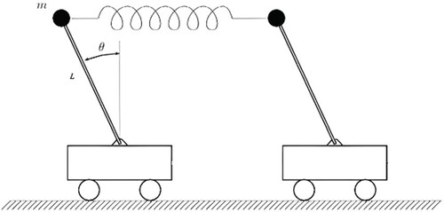
In this simulation, the masses of two pendulums chosen as $m_1=2kg$ and $m_2=2.5kg;$ the moments of inertia are $J_1=2kg.m^2$ and $J_2=2.5kg.m^2;$ the constant of the connecting torsional spring is $k=8N/m$; the length of the pendulum is $r=1m;$ the gravity constant is $g=9.8m/s^2$. Here, the sampling time is set as Ts = 0.1. We choose two local models, i.e. by linearizing the interconnected pendulum around the origin and $x_{i1}=(\pm {88}^{\circ },0)$, respectively, each pendulum can be represented by the following IT2 T-S fuzzy model with two fuzzy rules. (56) $\begin{array}{rl}& Rulel:IF{A}_{il}{x}_i(t)is{F}_i^{l}THEN\\ & {\dot{x}}_i(t)=\sum _{l=1}^r\sum _{j=1}^r{\tilde{w}}_{il}{\tilde{m}}_{ij}\\ & \times \left\{(A_{il}+B_{il}{G}_{ij})x_i(t)+D_{1il}{\omega }_i(t)+\sum _{\begin{array}{c}k=1\\ k\ne i\end{array}}^N{\overline{A}}_{ik}{x}_k(t)\right\}\\ & z_i(t)=\sum _{l=1}^p\sum _{j=1}^c{\tilde{w}}_{il}{\tilde{m}}_{ij}\{C_{il}{x}_i(t)+D_{2il}{\omega }_i(t)\}\end{array}$(56) where (57) $\begin{array}{rl}& A_{11}=\left[\begin{array}{cc}0& 1\\ 8.81& 0\end{array}\right],A_{12}=\left[\begin{array}{cc}0& 1\\ 5.38& 0\end{array}\right],{\overline{A}}_{12}=\left[\begin{array}{c}0\\ 0.25\end{array}\right],\\ & B_{1l}=\left[\begin{array}{c}0\\ 0.5\end{array}\right],D_{1l}=\left[\begin{array}{c}0\\ 0.5\end{array}\right],C_{1l}=[11]\end{array}$(57) for the first subsystem, and (58) $\begin{array}{rl}& A_{21}=\left[\begin{array}{cc}0& 1\\ 9.01& 0\end{array}\right],A_{22}=\left[\begin{array}{cc}0& 1\\ 5.58& 0\end{array}\right],{\overline{A}}_{21}=\left[\begin{array}{c}0\\ 0.20\end{array}\right],\\ & B_{2l}=\left[\begin{array}{c}0\\ 0.5\end{array}\right],D_{2l}=\left[\begin{array}{c}0\\ 0.5\end{array}\right],C_{2l}=[11]\end{array}$(58) for the second subsystem. Here, initial conditions are $x_1(0)=[1,-1{]}^T,x_2(0)=[1,-1{]}^T$ and ${\omega }_1(t)=0.8e^{-0.2t}\sin (0.2t)$ and ${\omega }_2(t)=0.6e^{-0.2t}\sin (0.2t)$. the sampling time is set as Ts = 0.1, so the sampling frequency would be fs = 10.

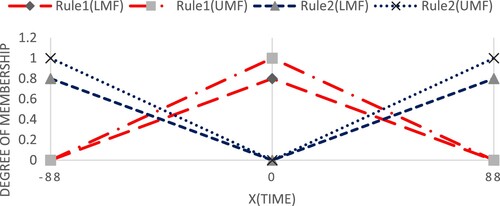
The two normalized triangular type-2 membership functions for two subsystem shown in Figure 2 are considered, where $r_i={88}^{\circ }$.

Figure 2. IT2 Membership function in Example.

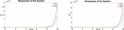
Remark 4.1

In this example, as it is clear by Figure 3, in the open loop case with no input vector, the system is not stable and trajectories of system are turned to the infinity. On the other hand, by applying the control system and making the closed-loop system, it will be evident by Figure 3 that trajectories of the system are converged to zero and proves the effectiveness of the algorithm.

Figure 3. State responses for open-loop double-inverted pendulums system.

Remark 4.2

One of the important issues in this paper is that external disturbances are considered permanently in this paper, and they are not applied on the specific time. They are considered from beginning to end and this shows the robustness of the proposed algorithm.

Remark 4.3

In comparison, in [33], a robust decentralized static output-feedback control is designed for a large-scale system which is modelled by Takagi–Sugeno and double inverted pendulum is proposed in the first example of the paper. As it is clear in [33], the trajectories of the pendulum are converged to zero after 10 sec. But in this paper, by proposed algorithm, as it is shown in Figure 3, trajectories of the inverted pendulum are converged to zero in about 4 sec that shows the strength of the proposed algorithm.

Remark 4.4

Considering the external disturbances ${\omega }_1(t)=0.8e^{-0.2t}\sin (0.2t)$ and ${\omega }_2(t)=0.6e^{-0.2t}\sin (0.2t)$, it can be seen that minimum of $H\mathrm{\infty }$ disturbance attenuation level ${\gamma }_{min}=0.333$ and the desired controller gains obtained in Table 1.

Table 1 Desired controller gains values for the double-inverted pendulum system.

$[G_{11}{G}_{12}{G}_{21}{G}_{22}]$	$\gamma$
$\left[\begin{array}{cccc}-34.3381& -60.0235& -174.0191& -485.0611\\ -16.2743& -31.7905& -93.5045& -268.4191\end{array}\right]$	$0.333$

Example 4.2

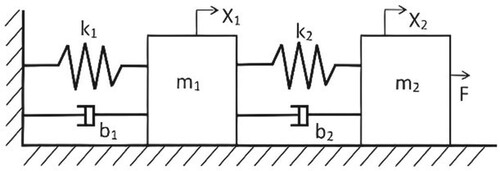
In this example, another large-scale system consisting of two subsystems is considered. Here, the proposed algorithm is applied to mass-spring-damper mechanical system due to [34]. For convenience, all parameters and configurations like the external disturbances, ${\omega }_1(t)=0.8e^{-0.2t}\sin (0.2t)$ and ${\omega }_2(t)=0.6e^{-0.2t}\sin (0.2t)$, are assumed same as the previous example. The mass-spring-damper mechanical system shown by Figure 4 is modelled in [34] and details of the modelling are existed. The mass-spring-damper mechanical system can be expressed by the following IT2 T-S fuzzy model with two fuzzy rules by linearizing the interconnected subsystems around the origin (Figure 5). $Rulel:IF{A}_{il}{x}_i(t)is{F}_i^{l}THEN$ $\begin{array}{rl}{\dot{x}}_i(t)& =\sum _{l=1}^r\sum _{j=1}^r{\tilde{w}}_{il}{\tilde{m}}_{ij}\{\phantom{\sum _{\begin{array}{c}k=1\\ k\ne i\end{array}}^N}(A_{il}+B_{il}{G}_{ij})x_i(t)+D_{1il}{\omega }_i(t)\\ & +\sum _{\begin{array}{c}k=1\\ k\ne i\end{array}}^N{\overline{A}}_{ik}{x}_k(t)\}\end{array}$ $z_i(t)=\sum _{l=1}^p\sum _{j=1}^c{\tilde{w}}_{il}{\tilde{m}}_{ij}\{C_{il}{x}_i(t)+D_{2il}{\omega }_i(t)\}$ $\begin{array}{rl}& A_{11}=\left[\begin{array}{cc}\begin{array}{c}-d_{11}/m_1\\ 1\end{array}& \begin{array}{c}-{\kappa }_1/m_1\\ 0\end{array}\end{array}\right],\\ & A_{12}=\left[\begin{array}{cc}\begin{array}{c}-d_{21}/m_2\\ 1\end{array}& \begin{array}{c}-{\kappa }_2/m_2\\ 0\end{array}\end{array}\right],{\overline{A}}_{12}=\left[\begin{array}{c}0.01\\ 0.02\end{array}\right]\end{array}$ $\begin{array}{rl}{A}_{21}& =\left[\begin{array}{cc}\begin{array}{c}-d_{11}/m_1-d_{12}{({\mathrm{\Omega }}_1)}^2\\ 1\end{array}& \begin{array}{c}-{\kappa }_1/m_1\\ 0\end{array}\end{array}\right],\\ A_{22}& =\left[\begin{array}{cc}\begin{array}{c}-d_{21}/m_2-d_{22}{({\mathrm{\Omega }}_2)}^2\\ 1\end{array}& \begin{array}{c}-{\kappa }_2/m_2\\ 0\end{array}\end{array}\right],\\ {\overline{A}}_{21}& =\left[\begin{array}{c}0.01\\ 0.03\end{array}\right]\end{array}$ $B_{11}=B_{12}=B_{21}=B_{22}=\left[\begin{array}{c}0.3\\ 0\end{array}\right]$ $D_{1l}=\left[\begin{array}{c}0\\ 0.5\end{array}\right],C_{1l}=[11]$ $D_{2l}=\left[\begin{array}{c}0\\ 0.5\end{array}\right],C_{2l}=[11]$here, due to [34], $m_1=m_2=1,{\kappa }_1=0.2,{\kappa }_2=0.3,d_{11}=0.6,d_{12}=0.8,d_{21}=0.5,d_{22}=0.7,{\mathrm{\Omega }}_1={\mathrm{\Omega }}_2=1$ and same as previous example, the sampling time is set as Ts = 0.1, so the sampling frequency would be fs = 10.

Figure 4. State responses for closed-loop double-inverted pendulums system.

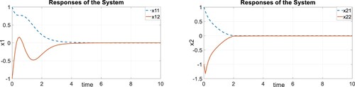
Figure 5. The mass-spring-damper mechanical system.

The two normalized type-2 sin membership functions for two subsystems shown in Figure 6 and Figure7, and the initial conditions are $x_1(0)=[1,-1{]}^T,x_2(0)=[1,-1{]}^T$.

with respect to [35] and by considering $\delta (x_i)=\sin (x_i)\in [-1,1],$ the membership functions for two subsystems and parameter uncertainties are: $\begin{array}{rl}& \{\begin{array}{l}{w}_i^1(z_{iq})=1-{\displaystyle \frac{1}{1+e^{x_i+4+\delta (x_i)}}}{w}_i^2(z_{iq})=1-w_i^1(z_{iq})\end{array},\\ & \{\begin{array}{l}{\underset{\_}{m}}_i^1(z_{iq})=1-{\displaystyle \frac{1}{1+e^{{\displaystyle \frac{-x_i-1.5}{2}}}}}{\overline{m}}_i^1(z_{iq})=1-{\displaystyle \frac{1}{1+e^{{\displaystyle \frac{-x_i+1.5}{2}}}}}{\underset{\_}{m}}_i^2(z_{iq})=1-{\overline{h}}_i^1(z_{iq}){\overline{m}}_i^2(z_{iq})=1-{\underset{\_}{h}}_i^1(z_{iq})\end{array},\\ & \{\begin{array}{l}{\underset{\_}{w}}_i^1(z_{iq})=1-{\displaystyle \frac{1}{1+e^{x_i+4-1}}}{\overline{w}}_i^1(z_{iq})=1-{\displaystyle \frac{1}{1+e^{x_i+4+1}}}{\underset{\_}{w}}_i^2(z_{iq})={\displaystyle \frac{1}{1+e^{x_i+4+1}}}{\overline{w}}_i^2(z_{iq})={\displaystyle \frac{1}{1+e^{x_i+4-1}}}\end{array}\end{array}$the mentioned parameter uncertainty is assumed as $\delta (x_i)=\sin (x_i)\in [-1,1],$ and ${\omega }_1(t)=0.8e^{-0.2t}\sin (0.2t)$ and ${\omega }_2(t)=0.6e^{-0.2t}\sin (0.2t).$ So we will have (Figures 6 and 7):

Figure 6. The membership function of IT2 fuzzy model. (a) The membership function of rule 2; (b) The membership function of rule 1.

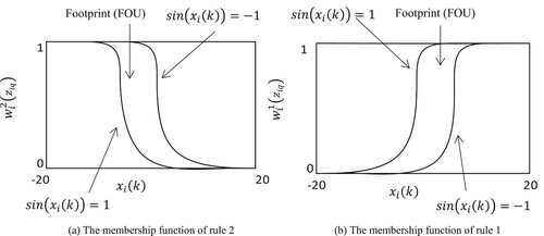
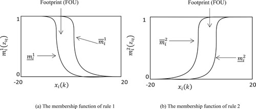
Figure 7. The membership function of IT2 fuzzy controller. (a) The membership function of rule 1. (b) The membership function of rule 2.

So, we have:

Remark 4.5:

With respect to Figure 8, although there are overshoots in state responses of the system, trajectories are converged to zero, asymptotically. This example, is presented in [34] and in comparison with, state responses of the system in [34] are converged to zero with many overshoots and undershoots after 20 Sec and illustrates the impracticality of the algorithm. Here, as it is demonstrated by Figure 8, trajectories converge in about 6 Sec and shows a dramatic difference between these two approaches.

Figure 8. State responses for mass-spring-damper.

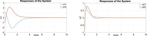
Remark 4.6:

Another important issue here that should be pointed out is computed gains shown in Table 2. By referring to this table, it is seen that computed gains have little value and this lessens costs of designing and computing. So, mass-spring-damper mechanical system is stabilized with a lower cost, and this is the efficient proposed approach.

Table 2 Desired controller gains values for the mass-spring-damper.

$[G_{11}{G}_{12}{G}_{21}{G}_{22}]$	$\gamma$
$\left[\begin{array}{cccc}-1.8665& -1.4405& -0.0683& -0.3894\\ -2.9733& -3.8023& -11.3970& -13.2382\end{array}\right]$	$0.333$

Remark 4.7:

This paper proposed a robust state feedback control for interval type-2 fuzzy Takagi–Sugeno large-scale systems. States of outputs can be identified by output feedback or by an observer and after that control signals are applied to stabilize them. Here, a problem is that this algorithm is not applicable for decentralized static output feedback systems and for those systems that states needed to be identified completely. These problems and limits must be investigated and solved for future works.

5. Conclusion

In this paper, the robust decentralized state feedback $H_{\mathrm{\infty }}$ type-2 fuzzy controller design has been investigated for continuous-time large-scale type-2 Takagi–Sugeno fuzzy systems. Through some linear matrix inequality techniques, it has been shown that the state fuzzy controller gain can be calculated by solving a set of LMIs. Then the resulting closed-loop fuzzy control system is asymptotically stable under extended dissipativity performance indexes. Uncertainties in the modelling of large-scale systems is the result of the using type-1 fuzzy Takagi–Sugeno model. Therefore, in this paper, the type-2 fuzzy model is used to cover modelling uncertainty for large scale systems. We also stabilized the large-scale system by using the type-2 fuzzy state feedback controller model with imperfect premise membership functions. The advantage of using membership function information in sustainability analysis is to reduce the conservatism of the obtained conditions. Then, in order to reduce the effect of external perturbations on the large-scale system, we applied the robustness control criterion name as extended dissipativity performance indexes to stability analysis, which was able to guarantee the $H_{\mathrm{\infty }}$ criterion, the $L_2-L_{\mathrm{\infty }}$, passive, and dissipativity performances. Finally, two numerical examples of double-inverted pendulum and mass-spring-damper mechanical system have been considered to verify the effectiveness of the developed methods. As it is clear, trajectories of systems are converged to zero in existence of the persistent disturbances, and this shows the robustness and effectiveness of the approach. Besides, the control vector is also converged to zero after sometimes that illustrates systems do not need input vector after trajectories enter a specified region and this improves the optimality of algorithm. The results of these simulations are to improve the control characteristics and make the conditions relax, as well as more complete coverage of the uncertainties in the system. can be mentioned weaknesses in this paper are those systems with time-varying delay. For these types of systems, the proposed algorithm in this paper is not valid. So, this approach must be revised in the future works. Besides, this approach is applied to state feedback and can be considered in future for systems with output feedback. An interesting problem for future research is to deal with the robust decentralized static output feedback $H_{\mathrm{\infty }}$ type-2 fuzzy control design for large-scale systems.

Disclosure statement

No potential conflict of interest was reported by the author(s).

Appendix

Assumption 1.

[36]

Let $\varphi ,{\psi }_1,{\psi }_2$ and ${\psi }_3$ be matrices such that the following conditions hold:

1. $\varphi ={\varphi }^T,{\psi }_1={\psi }_1^{T}and{\psi }_3={\psi }_3^T$;

2. $\varphi \ge 0$ and ${\psi }_1\le 0$;

3. $||D_{2_i}||.||\varphi ||=0;$

4. $(||{\psi }_1||+||{\psi }_2||).||\varphi ||=0;$

5. $D_{2_i}^T{\psi }_1{D}_{2_i}+D_{2_i}^T{\psi }_2+{\psi }_2^T{D}_{2_i}+{\psi }_3>0.$

Definition 1.

[36]

For given matrices $\varphi ,{\psi }_1,{\psi }_2$ and ${\psi }_3$ satisfying Assumption 1, system (5) is said to be extended dissipative if there exists a scalar $\rho$ such that the following inequality holds for any $t>0$ and all $\omega (t)\in {\mathcal{L}}_2[0,\mathrm{\infty })$: (A1) ${\int }_0^{t}J(s)dt-z^T(t)\varphi z(t)\ge \rho ,$(A1) where $J(t)=z^T(t){\psi }_{1}z(t)+2z^T(t){\psi }_{2}w(t)+w^T(t){\psi }_{3}w(t).$

It can be seen from Definition 1 that the following performance indexes hold.

1. Choosing $\varphi =0,{\psi }_1=-\mathit{I},{\psi }_2=0,{\psi }_3={\gamma }^2\mathit{I}$ and $\rho =0$ the inequality (59) reduces to the $H\mathrm{\infty }$ performance [13].

2. Let $\varphi =\mathit{I},{\psi }_1=0,{\psi }_2=0,{\psi }_3={\gamma }^2\mathit{I}$ and $\rho =0$ the inequality (59) becomes the $L_2-L_{\mathrm{\infty }}$(energy-to-peak) performance [14].

3. If the dimension of output $z(t)$ is the same as that of disturbance $w(t)$, then the inequality (59) with $\varphi =0,{\psi }_1=0,{\psi }_2=\mathit{I},{\psi }_3=\gamma \mathit{I}$ and $\rho =0$ becomes the passivity performance [15].

4. Let $\varphi =0,{\psi }_1=-ϵ\mathit{I},{\psi }_2=\mathit{I},{\psi }_3=-\sigma \mathit{I}$ with $ϵ>0$ and $\sigma >0$, inequality (59) becomes the very-strict passivity performance [16].

5. Let $\varphi =0,{\psi }_1=Q,{\psi }_2=S,{\psi }_3=R-\alpha \mathit{I}$ and $\rho =0$, inequality (59) reduces to the strict ($Q,S,R$)-dissipativity [17].

Lemma 1:

[37] (Jensen’s inequality)

For any constant positive semidefinite symmetric matrix $\text{W}\in {\mathit{R}}^{\mathit{n}\times \mathit{n}}$,${\text{W}}^{\text{T}}=\text{W}\ge 0$ two positive integers ${\text{d}}_2$ and ${\text{d}}_1$ satisfy ${\text{d}}_2\ge {\text{d}}_1\ge 1$ then the following inequality holds: ${\left(\sum _{k=d_1}^{d_2}x(k)\right)}^{T}W\left(\sum _{k=d_1}^{d_2}x(k)\right)\le \overline{d}\sum _{k=d_1}^{d_2}{x}^T(k)Wx(k)$where $\overline{d}=d_2-d_1+1$.

Lemma 2:

for given matrices $\overline{\mathrm{x}}\in {\text{R}}^{\text{n}}$, $\overline{\text{y}}$ and scaler $\kappa >0$ we have: $2{\overline{x}}^T\overline{y}\le {\kappa }^{-1}{\overline{x}}^T\overline{x}+\kappa {\overline{y}}^T\overline{y}$

References

- Liu Y, Liu X, Jing Y, et al. Annular domain finite-time connective control for large-scale systems with expanding construction. IEEE Trans Syst Man Cybern: Syst. 2020;51(10):6159–6169.
- Cao L, Ren H, Li H, et al. Event-triggered output-feedback control for large-scale systems with unknown hysteresis. IEEE Trans Cybern. 2020;51(11):5236–5247.
- Xin X, Tu Y, Stojanovic V, et al. Online reinforcement learning multiplayer non-zero sum games of continuous-time Markov jump linear systems. Appl Math Comput. 2022;412:126537.
- Sarbaz M, Zamani I, Manthouri M, et al. Hierarchical optimization-based model predictive control for a class of discrete fuzzy large-scale systems considering time-varying delays and disturbances. Int J Fuzzy Syst. 2022;24(4):2107–2130.
- Zhang J, Li S, Ahn CK, et al. Decentralized event-triggered adaptive fuzzy control for nonlinear switched large-scale systems with input delay via command-filtered backstepping. IEEE Trans Fuzzy Syst. 2021;30(6):2118–2123.
- Sarbaz M, Zamani I, Manthouri M. Fuzzy model predictive control contrived for type-2 large-scale process based on hierarchical scheme. 2020 28th Iranian Conference on Electrical Engineering (ICEE). 2020. IEEE.
- Bao L, Li Q, Lu P, et al. Execution anomaly detection in large-scale systems through console log analysis. J Syst Softw. 2018;143:172–186.
- Tan LN. Distributed H∞ optimal tracking control for strict-feedback nonlinear large-scale systems with disturbances and saturating actuators. IEEE Trans Syst Man Cybern: Syst. 2018;50(11):4719–4731.
- Sarbaz M, Soltanian MR, Manthouri M, et al. Adaptive optimal control of chaotic system using backstepping neural network concept. 2022 8th International Conference on Control, Instrumentation and Automation (ICCIA). 2022. IEEE.
- Sarbaz M, Manthouri M, Zamani I. Rough neural network and adaptive feedback linearization control based on Lyapunov function. 2021 7th International Conference on Control, Instrumentation and Automation (ICCIA). 2021. IEEE.
- Tanveer WH, Rezk H, Nassef A, et al. Improving fuel cell performance via optimal parameters identification through fuzzy logic based-modeling and optimization. Energy. 2020;204:117976.
- Lott GD, Da Silva MT, Cota LP, et al. Fuzzy decision support system for the calibration of laboratory-scale mill press parameters. IEEE Access. 2021;9:24901–24912.
- Zhang X, Wang H, Stojanovic V, et al. Asynchronous fault detection for interval type-2 fuzzy nonhomogeneous higher-level Markov jump systems with uncertain transition probabilities. IEEE Trans Fuzzy Syst. 2021;30(7):2487–2499.
- Lian Z, He Y, Zhang C-K, et al. Stability and stabilization of TS fuzzy systems with time-varying delays via delay-product-type functional method. IEEE Trans Cybern. 2019;50(6):2580–2589.
- Chaouech L, Soltani M, Chaari A. Design of robust fuzzy sliding-mode control for a class of the Takagi-Sugeno uncertain fuzzy systems using scalar sign function. Iran J Fuzzy Syst. 2020;17(5):97–107.
- Feng Z, Zhang H, Du H, et al. Admissibilisation of singular interval type-2 Takagi–Sugeno fuzzy systems with time delay. IET Control Theory Applic. 2020;14(8):1022–1032.
- Bahrami V, Mansouri M, Teshnehlab M. Designing robust model reference hybrid fuzzy controller based on LYAPUNOV for a class of nonlinear systems. J Intell Fuzzy Syst. 2016;31(3):1545–1564.
- Wang G, Jia R, Song H, et al. Stabilization of unknown nonlinear systems with TS fuzzy model and dynamic delay partition. J Intell Fuzzy Syst. 2018(Preprint): 1–12.
- Zhang Z, Zheng W, Xie P, et al. H-infinity stability analysis and output feedback control for fuzzy stochastic networked control systems with time-varying communication delays and multipath packet dropouts. Neural Comput Appl. 2020;32:14733–14751.
- Yuan K, Li W, Xu W, et al. A comparative experimental evaluation on performance of type-1 and interval type-2 Takagi-Sugeno fuzzy models. Int J Mach Learn Cybern. 2021;12(7):2135–2150.
- Chang W-J, Lin Y-W, Lin Y-H, et al. Actuator saturated fuzzy controller design for interval type-2 Takagi-Sugeno fuzzy models with multiplicative noises. Processes. 2021;9(5):823.
- Júnior MP, da Silva MT, Guimarães FG, et al. Energy savings in a rotary dryer due to a fuzzy multivariable control application. Drying Technol. 2020;40(6):1196–1209.
- Su H, Zhang H, Liang X, et al. Decentralized event-triggered online adaptive control of unknown large-scale systems over wireless communication networks. IEEE Trans Neural Network Learn Syst. 2020;31(11):4907–4919.
- Farina M, Scattolini R. Distributed MPC for large-scale systems. In: Handbook of model predictive control. Springer; 2019. p. 239–258.
- Zhao P, Alizadegan A, Nagamune R, et al. Robust control of large-scale prototypes for miniaturized optical image stabilizers with product variations. 2015 54th Annual Conference of the Society of Instrument and Control Engineers of Japan (SICE). 2015. IEEE.
- Mir AS, Bhasin S, Senroy N. Decentralized nonlinear adaptive optimal control scheme for enhancement of power system stability. IEEE Trans Power Syst. 2019;35(2):1400–1410.
- Shanmugam L, Joo YH. Stability and stabilization for T–S fuzzy large-scale interconnected power system with wind farm via sampled-data control. IEEE Trans Syst Man Cybern: Syst. 2020;51(4):2134–2144.
- Sabzalian MH, Mohammadzadeh A, Lin S, et al. A robust control of a class of induction motors using rough type-2 fuzzy neural networks. Soft comput. 2020;24(13):9809–9819.
- Zhang J, Chen W-H, Lu X. Robust fuzzy stabilization of nonlinear time-delay systems subject to impulsive perturbations. Commun Nonlinear Sci Numer Simul. 2020;80:104953.
- Feydi A, Elloumi S, Braiek NB. Robust decentralized optimal stabilizability of continuous time uncertain interconnected systems: application to large scale power system. Optim Control Appl Methods. 2022;43(6):1604–1622.
- Cheng P, Wang H, Stojanovic V, et al. Asynchronous fault detection observer for 2-D Markov jump systems. IEEE Trans Cybern. 2021;52(12):13623–13634.
- Xu Z, Li X, Stojanovic V. Exponential stability of nonlinear state-dependent delayed impulsive systems with applications. Nonlinear Anal Hybrid Syst. 2021;42:101088.
- Zhong Z, Zhu Y, Yang T. Robust decentralized static output-feedback control design for large-scale nonlinear systems using Takagi-Sugeno fuzzy models. IEEE Access. 2016;4:8250–8263.
- Kim HJ, Park JB, Joo YH. Decentralized H∞ fuzzy filter for nonlinear large-scale sampled-data systems with uncertain interconnections. Fuzzy Sets Syst. 2018;344:145–162.
- Sarbaz M, Zamani I, Manthouri M, et al. Decentralized robust interval type-2 fuzzy model predictive control for Takagi–Sugeno large-scale systems. Automatika. 2022;63(1):49–63.
- Zhang B, Zheng WX, Xu S. Filtering of Markovian jump delay systems based on a new performance index. IEEE Trans Circuits Syst Regul Pap. 2013;60(5):1250–1263.
- Jiang X, Han Q-L, Yu X. Stability criteria for linear discrete-time systems with interval-like time-varying delay. Proceedings of the 2005, American Control Conference, 2005. 2005. IEEE.
Appendix
Assumption 1.
[Citation36]
Let and
be matrices such that the following conditions hold:
Definition 1.
For given matrices and
satisfying Assumption 1, system (5) is said to be extended dissipative if there exists a scalar
such that the following inequality holds for any