Real-time NIR camera brightness control using face detection

Abstract

The face image analysis field is a well-established research area in computer vision and image processing. An important requirement for accurate face image analysis is a high-quality input face image. In different real-life scenarios, however, the face is often not properly illuminated, which makes the face analysis very difficult or impossible to accomplish. Although a better performance is obtained by changing the spectrum from visible to near-infrared, it is still not enough for extreme illumination conditions. To obtain a high-quality near-infrared face image, a fast automatic brightness control method using approximate face region detection is proposed, which properly adjusts the brightness of the face part of the image. A novel algorithm for approximate face region detection based on spatio-temporal sampled skin detection is proposed together with the split-range feedback controller and the face absence handle. The proposed method is much faster than state-of-the-art solutions and accurate in approximate face region detection. The complete execution time is lower than 10 milliseconds which makes it suitable for hard real-time embedded system implementation and usage, while the reference brightness value is achieved within 10–15 frames, making it robust to extreme illumination conditions in a scene.

Keywords:

• Near-infrared images
• automatic brightness control
• face detection
• split-range feedback control
• embedded systems
• real-time image processing

1. Introduction

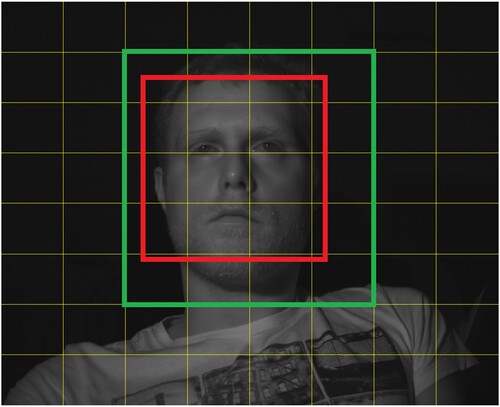
Face image analysis is one of the most active fields in the computer vision field. To extract useful information from images or videos, a high-quality input image is needed for various computer vision tasks so that the face would be recognized in the scene. The recent research shifts the focus from the visible light spectrum (VIS) to the near-infrared spectrum (NIR) because of the high skin reflectance of the near-infrared light which allows better performance while low illumination is present, as seen in Figure 1.

Figure 1. Image of a face captured in the near-infrared spectrum.

However, it is not enough to change the spectrum to get a proper face image. While NIR image enhancement is thoroughly explored, enhancing a poorly captured image can be a very demanding task, and often important information can't be recovered. This is the result of noise, overexposure, and underexposure from the high-dynamic scene range or different lighting scenarios. An alternative approach to this problem is to change the brightness of the scene, and this is done with automatic brightness control. The main task of automatic brightness control is to properly adjust the scene brightness through the camera's internal hardware design and/or external illumination source. Changing the brightness of the whole scene or static region of interest (ROI) with a face consists of the brightness calculation of both the face and a large amount of background. If the face moves outside the scene or the static ROI, the brightness will suddenly change which directly affects the brightness control behavior and result. The algorithm will try to compensate for the change which will often bring the hardware to its limits. The dynamic ROI helps the algorithm to achieve the proper performance. For this reason, the automatic brightness control for face analysis in the near-infrared spectrum with approximate face region detection is introduced. The proposed method provides a fast, precise, and resourceful solution to rectify the face brightness allowing it to be recognized with the other face analysis algorithms by analyzing only the face region and changing the brightness of the whole scene according to the face region brightness.

The two major contributions of this paper are as follows:

• Real-Time Spatio-Temporal Method for Approximate Face Region Detection in NIR Spectrum: the approximate face region detection optimized for the embedded systems which also includes the previous region position,

• Automatic Brightness Control Method based on the Split-Range Feedback Control with Approximate Face Region Detection Optimized for Embedded Systems: The image acquisition in the system is a multiple-input single-output (MISO) system in which the proposed approximate face detection method is used.

To the best of the authors' knowledge, the proposed methods and the implementations have not been presented in the literature before.

The paper is organized as follows: in Section 2 related work in automatic brightness control and face detection in the NIR spectrum is presented. Furthermore, in Section 3, the proposed methods for automatic brightness control and approximate face region detection are discussed, together with the system and hardware overview. In Section 4, experiment results are presented to evaluate algorithm performance. In Section 5, a discussion of the paper is introduced and, finally, the conclusion is given in Section 6.

2. Related work

Automatic brightness control is a well-researched topic in control systems. There are several approaches to control the scene brightness like model approach [1], machine learning approach [2] and deep learning approach [3]. The model-based approach needs to have an adequately estimated model to give good results which is a demanding task for approximating non-linear models such as brightness change in a scene. In this situation, a machine-learning-based and deep-learning-based strategy can be used, but a large dataset with annotated videos is needed, which is a significant drawback. Another popular approach to get the proper luminance of the scene is the feedback control system and the most common feedback control system is the Proportional-Integral-Derivative (PID) controller [4]. The PID controller offers fast convergence to the target value if appropriately tuned. Mean pixel value is the common scene brightness measure in which the average brightness of the whole image or the specific ROI is calculated [4].

In the usual approach, the camera inputs are changed one at a time, which can lead to the complex parameter tuning process in multiple-input-single-output (MISO) systems like image acquisition systems and in slower convergence. However, in [5], the camera inputs are controlled simultaneously with the split-range feedback control system.

Using a whole image often slows the face analysis algorithms. Moreover, the fixed region information contains face and background information, so the result of the region analysis is not always the proper representation of the face, especially if the face is moving in the scene, so the dynamic face region calculation is needed. The dynamic face region calculation should also be a lightweight process because it is used in embedded systems in real time. The most common method for face detection is the Viola-Jones face detection algorithm [6]. While its face detection rates are high, it tends to be slow for real-time execution [7], especially on the embedded system. Another popular toolkit used for face detection is dlib [8], an open-source library and it also isn't appropriate for the embedded system implementation. Background/foreground segmentation is also used to determine the face region. In [9], a fixed threshold is used to detect the background, while in [10] the face area is calculated by finding the biggest area after image binarization by automatic threshold determination using the discriminant analysis method using stereo cameras. A fixed threshold is not suitable for high dynamic scenes while using a second camera increases the hardware complexity and introduces a need for additional synchronization between cameras and the embedded system. In [11], Otsu's method for thresholding [12] with horizontal and vertical projection is used for face detection. Horizontal and vertical projection calculations tend to be slow and not as precise as the other methods. In [13], a cascade random forest classifier with oriented center-symmetric local binary patterns is employed, while in [14] Multi-Task Cascaded Convolutional Neural Network (MTCNN) is used. Regarding the embedded system implementation, most algorithms are Viola-Jones-based. While those methods are very accurate in face region detection, the execution time on the embedded system in real-time is difficult and often impossible without powerful hardware.

Several solutions combined face region detection and automatic brightness control in the NIR spectrum. In [15], the face is detected by the skin detection method which includes Otsu's method for threshold calculation and vertical and horizontal projections in an image from a fusion of two NIR bands, while the luminance adjustment is based on a lookup operation at the Luminance-Voltage diagram. In [16], a precalculated face image mask is used to emphasize the most important face regions, and the brightness is changed by adding/subtracting precalculated exposure and gain discrete values. The main problem of the two methods is that the automatic brightness control is very rudimental which often results in slow convergence or even oscillations around the reference value, which is not the wanted system behavior. A brief comparison overview of the proposed methods can be seen in Table 1.

Table 1. Comparison of the different automatic brightness control algorithms used in real-time embedded systems with Viola-Jones face detection algorithm included.

Algorithm	Automatic brightness control execution	Face region detection execution	Past region locations included in calculation
Vugrin [5]	Fast convergence	–	–
Dowdall [15]	Slow convergence	Medium accuracy, Slow	No
Gnatyuk [16]	Slow convergence	Medium accuracy, Slow	No
Viola-Jones [6]	–	Very High accuracy, Slow	No
Proposed method	Fast convergence	High accuracy, Fast	Yes

Many different algorithms are implemented for automatic brightness control. However, the inclusion of face region detection greatly reduces the number of publications, especially in the NIR spectrum. Moreover, the control algorithms are often focused on one parameter at a time. In this paper, the automatic brightness control with simultaneous control of camera parameters with approximate face region detection is introduced.

3. Proposed method for automatic brightness control with approximate face region detection

The current state-of-the-art automatic brightness control algorithms with face detection for the embedded system often struggle with performance and/or execution time. To surpass the given bottleneck, a split-range controller with approximate spatio-temporal face region detection is introduced. In Figure 2, the proposed system scheme is presented. The orange rectangle contains the automatic brightness control part consisting of a split-range PID controller, anti-windup, and clipping mechanism, while the blue blocks represent approximate face region detection with handling the face absence in a scene. Firstly, the split-range controller is described thoroughly. After that, the approximate face region detection algorithm is introduced.

Figure 2. Split-range PID controller block scheme with Automatic Brightness Control (orange) with Anti-Windup, Clipping Mechanism, and Time Delay Block $-d$ and Approximate Spatio-Temporal Face Region Detection (blue) with Face Absence Handle.

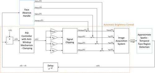
3.1. Split-range feedback controller

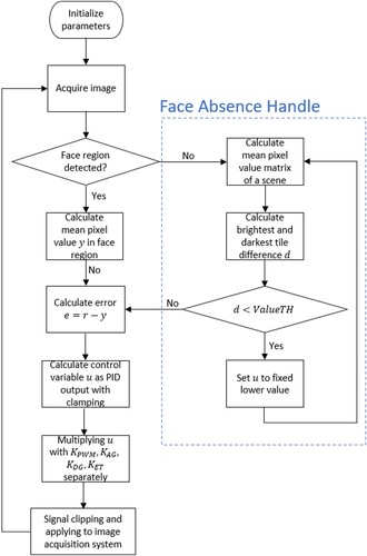
The PID controller is the most common feedback controller used in engineering [4]. In the orange rectangle in Figure 2, the proposed PID control scheme is presented, while the flowchart of the algorithm can be seen in Figure 3. The main signal of the PID controller is error term e which is the difference between reference value r and the current measured mean pixel value y, calculated from the histogram of intensities in the ROI. There are three components in the PID controller: proportional (P), integral (I), and derivative (D) term. The proportional part, as its name states, is directly proportional to the error term. The integral part is the sum of all the previous errors that occur during the control process, while the derivative part is the difference between the current and previous error terms. The ideal PID controller discretized with the backward Euler method in parallel form is shown in (1(1) $u\left(k\right)=K_{p}e\left(k\right)+K_i{T}_s\sum _{i=0}^{k}e\left(i\right)+\frac{K_d}{T_s}\left[e\right(k)-e(k-1\left)\right],$(1) ): (1) $u\left(k\right)=K_{p}e\left(k\right)+K_i{T}_s\sum _{i=0}^{k}e\left(i\right)+\frac{K_d}{T_s}\left[e\right(k)-e(k-1\left)\right],$(1) where u is the control variable in k-th step, $K_p$, $K_i$ and $K_d$ are proportional, integral and derivative coefficients respectively and $T_s$ is sampling time. The sampling time is often embedded in the mentioned coefficients. The process of adjusting P, I, and D gains is called parameter tuning and the response of the system highly depends on the coefficients chosen. There is extensive research in control theory about tuning the parameters for linear systems. However, as it is mentioned before, the image acquisition system is non-linear and, therefore, a different approach is needed. The system can be linearized at the operating point, but for that precise mathematical model is needed. In this camera system, four different controllable inputs affect the brightness of a scene: the external illumination source controlled with PWM, analog gain (AG), digital gain (DG), and exposure time (ET). For that reason, four control signals are used in this system: $u_{PWM}$ is the infrared illumination source control signal, $u_{AG}$ is the analog gain control signal, $u_{DG}$ is the digital gain control signal and $u_{ET}$ is the exposure time control signal. Building a model that consists of four non-linear and mutually dependent subsystems is not an easy task. To reduce the complexity of the system, the joint control variable u is used. The variable u is a direct output from the controller which is then propagated to the four control signals through the respective gains $K_{PWM}$, $K_{AG}$, $K_{DG}$ and $K_{ET}$ which weight the impact on the image acquisition system, respectively. Instead of tuning twelve different parameters (four PID controllers with each having three gains), the number of parameters is reduced to eight tunable parameters. $K_{PWM}$, $K_{AG}$, $K_{DG}$, and $K_{ET}$ gains need to be tuned properly. Produced infrared illumination needs to be dominant, so the emphasis should be on $K_{PWM}$, while $K_{AG}$ and $K_{DG}$ need to be at lower values. $K_{ET}$ needs to be chosen properly so that ambient light is not very expressed while preserving the overall brightness of the face region. The mean pixel value is calculated for each tile in an 8×8 grid. If the face region is not detected, the face absence handle activates. The two most often scenarios that can cause this behavior is camera covering or the face moving out of the scene boundaries. If the difference between the brightest and the darkest mean pixel value tiles d is lower than the threshold value ValueTH, the difference between classes is too small to properly identify the background and the foreground. The joint control value u is set to a fixed lower value. In that way, a lower mean pixel value is achieved and the sudden potential ambient light change is compensated, but it is high enough to detect the reappeared face region.

Figure 3. Flowchart of the automatic brightness control part with face absence handle.

3.2. Approximate face region detection

The main task of the automatic brightness control in this paper is to obtain a proper brightness of a face. In most cases, the face is in a part of a scene and not in the whole image, so face detection is needed to isolate the part of the image with the face included to get the actual face brightness. However, face detection is a complex and often slow task for embedded systems, especially as a neural network solution, so a good representation of face brightness is needed. Instead of using the face for the automatic brightness control approximate face region is introduced as a substitute. The approximate face region calculation is fast, approximately accurate, and adjusted for the implementation on the embedded real-time system. Exact face detection is not necessary, mostly because many implementations on embedded systems divide the scene into x rows and y columns. The major requirement, however, is the stability of the calculated region. Head movements are not big between two frames at 30 frames per second (fps) in normal behavior so the region should not change drastically between two frames. In this paper, the approximate face region detection is based on the spatio-temporal sampled skin detection in the scene regions to separate the potential face region from the background.

3.2.1. Spatio-Temporal sampled skin detection

The spatio-temporal sampled skin detection uses the embedded system property of dividing the image into rows and columns and calculating the statistics for each region separately. It is fast and no dataset is needed, but it tends to be less accurate than some commonly used face detection algorithms due to extreme lighting conditions, clothes color, etc. There are multiple instances of the algorithm, as shown later in the paper. The beginning of the spatial step of the algorithm is common, as can be seen in the workflow in Figure 4.

Figure 4. Flowchart of the spatial step of the spatio-temporal sampled skin detection.

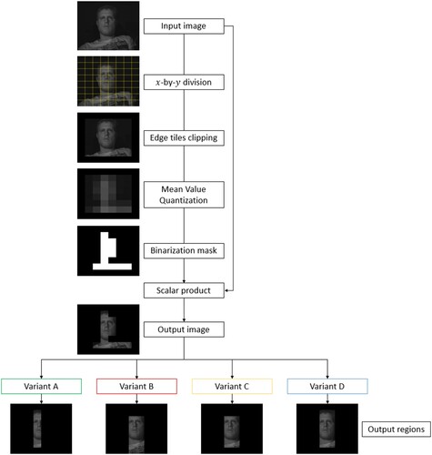
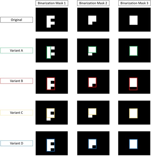
After the image acquisition, the image is divided into x rows and y columns. In this example, both x and y are equal to 8. The edge tiles are ignored due to the low probability of detecting faces in them. The mean pixel value in every tile is calculated and the x−2-by-y−2 matrix is formed. The matrix is then binarized with the threshold determined by Otsu's method [12] and the binarized mask is created. At this point, the algorithm is split into four variants. After the binarization, the biggest vertical rectangle or squares of positive values is searched for in the matrix, and that is the first variant, A. In the second variant, B, the biggest rectangle with a percentage of the positive values greater or equal to 75% of the rectangle size is chosen as the face region. The third variant, C, changes negative values to positive if they are surrounded by more than 50% of positive values (more than 4) first and then calculates the biggest vertical rectangle or square as in Variant A.

The final variant, D, also uses the rectangle from variant A and expands it to the neighboring columns left and right to the rectangle if the percentage of positive values in each column is greater or equal to 50% of the total number of values in the column. In Figure 5, the bounding boxes from the variants are presented, while in Figure 6 the behavior of the variants is shown for three different artificial binarization masks. The regions can also be expanded by 1 in every direction, if possible.

Figure 5. The bounding boxes of the spatial step variants of the spatio-temporal sampled skin detection.

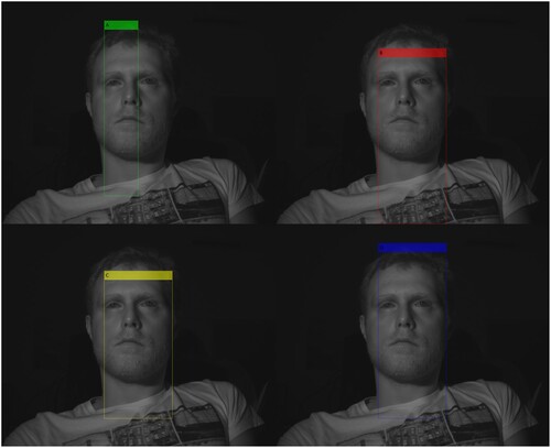
Figure 6. Approximate face regions obtained by the four variants for three different artificial binarization masks.

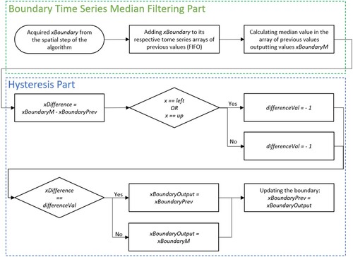
After the spatial step of the detection finishes, the calculated region boundaries go through the temporal step of the spatio-temporal sampled skin detection. The temporal step consists of two parts, as shown in the workflow in Figure 7. Firstly, the boundary time series median filtering is used. For every of the four region boundaries, a new calculated boundary from spatial step xBoundary is added to the array of the k−1 previous boundary values by the First-In-First-Out (FIFO) principle, and the median value is chosen for the further calculation, xBoundaryM. As stated, the face movement between two frames at 30 fps is often small, so the region boundary oscillations should also be minimal. The boundary time series median filtering is used to prevent the potential sudden big changes in boundaries due to extreme light conditions, covering the face, or similar occurrences. The second step is hysteresis. If the face slightly moves in a new region, it occurs only in a small part of the new tile and the rest is background, but it is still included in the calculation. For this reason, the value xBoundaryM is compared with the previous value of that boundary, xBoundaryPrev. The difference between the two values, xDifference is compared to the value differenceVal, which is -1 if the xBoundary is the left or the up boundary, or 1 if it is the right or down boundary. If that is the case, the hysteresis stops the region expansion and the output boundary xBoundaryOutput is set to the previous value xBoundaryPrev, and, if not, it is set to calculated median xBoundaryM. Finally, the boundary values are updated and xBoundaryOutput is stored to xBoundaryPrev which ends the current iteration.

Figure 7. Flowchart of the temporal step for the one boundary of the spatio-temporal sampled skin detection.

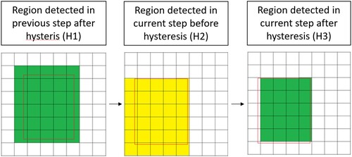
In Figure 8, the hysteresis effect is presented visually. In the H1 part, the red rectangle represents the actual face position, while the green tiles represent the calculated face region in the previous step. In H2, the face moves slightly to the left and down, and the calculated region is also moved in the same direction. The face region is colored yellow. In H3, the hysteresis is calculated and the face region is reduced. The left and down boundary movement would enlarge the region, so the hysteresis reverts it to the previous values. The right and the up boundary also change, but the region is not increased by it so no change in those boundaries occurs. The previous region in hysteresis doesn't need to be the same as the one in the boundary time series array due to hysteresis in the previous step.

Figure 8. Hysteresis effect on the region expansion attempt.

The order in the temporal step doesn't need to be the same, the boundary time series median filtering and hysteresis can switch places and be used independently. However, both the boundary time series median filtering and hysteresis are non-linear operations so the result could differ from the described algorithm. In Algorithm 1, the whole algorithm is shown which includes the automatic brightness control with a split-range controller and real-time spatio-temporal approximate face region detection with expansion, time series median filtering, and hysteresis calculation. There is an option to find some values with an optimization algorithm, such as the number of previous steps in boundary time series median filtering and the percentages for Variant B, C, and D. However, the optimization algorithm is not necessary for those values because most the values are unsigned integer numbers that are easily determined by a simple visual inspection, such as the previous step number. Regarding the percentages of the variants, they were discovered heuristically by analyzing the incomplete rectangular ROI shapes to find the rules to enclose the biggest rectangle. The grid size dimensions are also limited to small unsigned integer values, otherwise, the mean pixel calculation in a region would not be useful compared to the mean pixel value calculation of the whole image. Finally, the image binarization threshold is calculated with Otsu's method which determines the optimal value for the threshold.

In Section 4, experiments and results are shown to evaluate system and algorithm performance.

4. Experiments and results

The proposed automatic brightness control with approximate face region detection needs to be evaluated. Many experiments were conducted to determine if the algorithm works as described. The experiments are divided into three parts. In the first part, the evaluation and the comparison of the approximate face region detection are made. In the second part the execution time of the algorithm on the embedded system is measured, while in the last part, the overall dataset system evaluation of approximate face region detection and automatic brightness control is made.

4.1. Approximate face region detection evaluation

Face and face region detection are best tested on a benchmark dataset. In this case, the needed dataset should contain the infrared face videos captured during the day and night. There are several datasets available, but many of them are not annotated. The dataset that covers all the criteria is the face alignment data set used in driving (FADID) [17]. The dataset was constructed for facial landmark detection under real driving situations which consist of changes in pose change, illumination change, and partial occlusions from hair or sunglasses. The resolution of the images is 720×480. The dataset contains the test and the training set for both the daytime (3327 images) and the nighttime (2583 images). However, the proposed algorithm is learning-free, so the training sets can also be used in the algorithm testing. The daytime training set is divided into six batches: images from 00001–00260, 00261–00517, 00518–00735, 00736–00971, 00972–01243, and 01244–01493, while the nighttime training set is divided into four batches: images from 0001–00193, 00194–00397, 00398–00581 and 00582–00862, however, images 00796–00862 weren't used in the calculation because of the sequence discontinuance at images 00796 and 00826. The facial landmarks are annotated together with the face location containing the top-left and bottom-right coordinates. However, the nighttime test set was not properly annotated and it needed to be done again by hand in which the previous annotation procedures were followed to obtain similar face boundaries. The results of the algorithm were compared to the most common face detection method used for the embedded system implementation – the Viola-Jones face detection algorithm. The algorithm is based on calculating the face region, so the bounding boxes in which the face is located are expanded to the region boundaries, as shown in Figure 9.

Figure 9. The face bounding box (red) expanded to the face region bounding box (green).

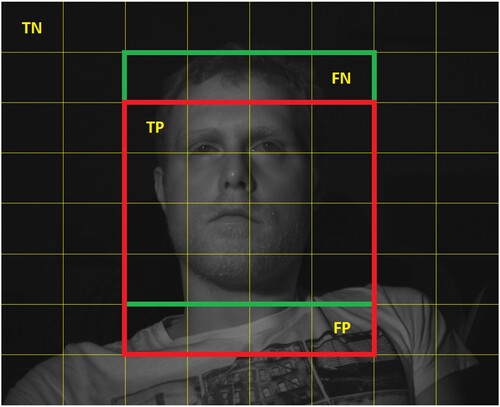
This is done for the Viola-Jones algorithm and for annotated faces, which are then used as the ground truth. If the tiles marked as a part of the face region are overlapping for the ground truth and the algorithm, they are marked as true positive. If the background tiles are overlapping for the ground truth and the algorithm, they are marked as true negative. If the algorithm detects the face region outside the ground truth region, it is marked as a false positive, while if the algorithm doesn't detect the ground truth region, it is marked as a false negative. This is shown in Figure 10.

Figure 10. Overlapping ground truth face region (green) and detected face region (red) with examples of true positive (TP), true negative (TN), false positive (FP) and false negative (FN).

Standard quality metrics are used for evaluating the binary classification tasks: accuracy, precision, recall, and F1-score. For this experiment, an 8×8 grid is used for computation due to the embedded system usage in the next experiment. There are a total of 136 subvariants of the spatio-temporal algorithm for approximate face region detection tested. All four variants(A, B, C, D) are calculated with and without expansion, and with and without temporal step. All four subvariants of the temporal step are also used (hysteresis only, time-series median filtering only, first hysteresis, then time series median filtering, and first time series median filtering then hysteresis). The window sizes for the time series median filtering are 3, 5, 11, 15, and 29. In Table 2, accuracy, precision, recall, and F1-score are shown for the Viola-Jones algorithm and the five best-performed variants in the daytime, nighttime and overall dataset. As seen in Table 2, the Viola-Jones algorithm outperforms all the variants in face region detection. However, the difference is not as significant as expected. The biggest difference can be seen in the daytime recordings where Viola-Jones is better, but some variants outperform the Viola-Jones algorithm in the nighttime. The variant name consists of one of the four variants (A, B, C, or D). Then, the expansion option follows separated with the underscore, Expn0 means expansion isn't present, while Expn1 means that the calculated region is expanded in every direction by 1. After another underscore, the number with the prefix T means the window size in the time series median filtering. If the number is 00, the time series median filtering isn't performed. The last part consists of two letters and four possible combinations. HO means that only the hysteresis is performed, while TO means only time series median filtering is performed. If the letter sequence is HT, firstly hysteresis and then time series median filtering is performed and, if it is TH, the operation order is switched. The example A_Expn1_T03_TH means that variant A is used with region expansion Expn1 in which firstly the time series median filtering is calculated followed by hysteresis (TH) with the window size 3 (T03). The best results were obtained with variant A with expansion using only hysteresis, combined hysteresis, and time series median filtering with window sizes 3 and 5. In this case, regardless of the order of the hysteresis and time series median filtering, the results were the same.

Table 2. Face region detection accuracy, precision, recall, and F1-score comparison between Viola-Jones face detection and the five best-performed proposed method variants in the daytime, nighttime and total.

	Accuracy (%)			Precision (%)			Recall (%)			F1-Score (%)
Algorithm	Day	Night	Total	Day	Night	Total	Day	Night	Total	Day	Night	Total
Viola-Jones	89.02	89.13	89.07	55.87	59.29	57.37	89.89	90.05	89.96	66.89	69.96	68.24
A_Expn1_T00_HO	81.27	89.68	84.95	44.29	67.81	54.57	88.91	84.40	86.94	57.95	71.65	63.94
A_Expn1_T03_HT	81.09	88.96	84.53	43.96	66.75	53.92	89.30	84.82	87.34	57.80	70.80	63.48
A_Expn1_T03_TH	81.09	88.96	84.53	43.96	66.75	53.92	89.30	84.82	87.34	57.80	70.80	63.48
A_Expn1_T05_HT	80.93	88.84	84.39	43.81	65.75	53.40	89.72	85.30	87.79	57.75	70.65	63.39
A_Expn1_T05_TH	80.93	88.84	84.39	43.81	65.75	53.40	89.72	85.30	87.79	57.75	70.65	63.39

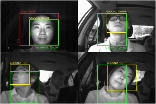
Figure 11 shows interesting examples from the FADID dataset in which the approximate face region detection has been executed. The ground truth bounding box is yellow, the proposed variant $A\mathrm{\_}Expn1\mathrm{\_}T\mathit{00}\mathit{\_}\mathit{H}\mathit{O}$ bounding box is green and the Viola-Jones bounding box is red. In the upper-left example, ground truth and proposed variant regions are the same, so the proposed algorithm has worked well for this case. But, in other examples, this is not the case. As seen from Figure 11, the biggest obstacle for the face region detection performance is the color of the clothing or the reflectance of the clothes. However, the region does not move often and the face is included in it, which is beneficial for the automatic brightness control system where the region position stability is as important as the face region detection. It can also be seen that the proposed variant works well with the different face poses. The same statement can not be said for the Viola-Jones algorithm. Viola-Jones algorithm searches for patterns, and different face poses cause the difficult or even impossible to detect the face region, which is the case for the upper-right and image examples in the second row in Figure 11. The frontal faces with occlusion, such as glasses, are well detected with both Viola-Jones and the proposed method. The FADID dataset lacks images with extreme lighting conditions, so no conclusion can be made for the face region detection in this type of scene.

Figure 11. FADID dataset approximate face region detection examples with ground truth bounding box (yellow), proposed variant $A\mathrm{\_}Expn1\mathrm{\_}T\mathit{00}\mathit{\_}\mathit{H}\mathit{O}$ bounding box (green) and Viola-Jones bounding box (red), including the examples in which the algorithm doesn't perform well.

4.2. Approximate face region detection execution time measurement on the embedded system

After the experiment in which the face region detection capability had been tested, the performance of the approximate face region detection was examined in the target embedded system. In this subsection, the efficiency of the algorithm variants was measured. The main goal of the experiment was to measure the execution time in which the face region was detected. The embedded system used for the evaluation is Xilinx Zynq UltraScale+ MPSoC ZCU104 Evaluation Kit. The images used for measuring execution time were from FADID dataset [17] from the test_ej_1 folder. The measurement and comparison were done between the Viola-Jones algorithm and worst-case scenario for every variant with region expansion and both hysteresis and time series median filtering calculation with windows size 29. The results are shown in Table 3. The parameter specifying how much the image size is reduced at each image scale is the scale factor of the Viola-Jones algorithm.

Table 3. The average execution time comparison on the Xilinx ZCU104 between the Viola-Jones algorithm with a scale factor 2.5 and worst-case scenario for every variant.

	Average execution time (milliseconds)
Viola-Jones – scale factor 2.5	41.65
Worst case scenario (variant A)	1.62
Worst case scenario (variant B)	1.62
Worst case scenario (variant C)	1.65
Worst case scenario (variant D)	1.62

A higher scale factor results in a faster execution [18], but with a higher chance of face not being detected, and vice versa. As seen in [18], a scale factor up to 2 is used. The scale factor was set to 2.5, which is an exaggerated value to emphasize how the Viola-Jones algorithm is slow in comparison to the proposed method, even with an extreme value such as 2.5.

As seen in Table 3, the Viola-Jones algorithm is much slower than any of the proposed variants. The calculation time didn't include image reading, mean pixel value calculation, and converting to a grayscale image as those are often part of the system's image processing pipeline. While the mean pixel value executes fast, the image loading/capturing can consume a lot of time if it is not implemented properly. The last part of the experiments is the evaluation of the automatic brightness control approximate face region detection in the embedded system.

4.3. Automatic brightness control with approximate face region detection

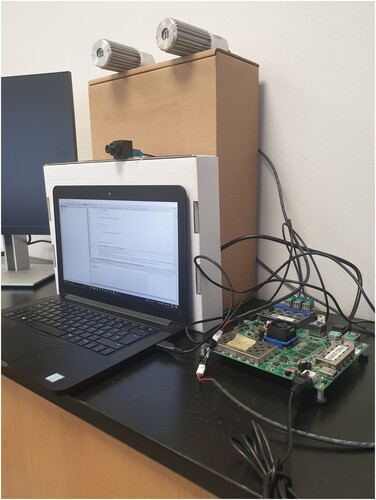
The last experiment evaluated the automatic brightness control with the split-range controller with spatio-temporal approximate face region detection on the embedded system. The experiment was conducted in a laboratory, where real-world scenarios were simulated. The image acquisition system consisted of Xilinx Zynq UltraScale+ MPSoC ZCU104 Evaluation Kit, OmniVision OV2311 image sensor with cut-off 940 nm filter, and two illumination sources with infrared light-emitting diodes (IR LED) with a wavelength of 940 nm. The setup can be seen in Figure 12. There were several constraints like system delay, the frame rate of 30 frames per second (fps), and image division in 8×8 equal tiles. The main idea of the laboratory tests was to examine the convergence speed and the presence of the oscillations in the mean pixel value signal while achieving the proper face luminance. PID parameters were tuned by [4], where $K_i$ is set relatively high to $K_p$, so the mean pixel value gradually reaches the target value.

Figure 12. The image acquisition system setup including Xilinx ZCU104 board, OmniVision OV2311 image sensor, and two infrared illumination sources.

The disturbance caused by the ambient light was simulated with a second infrared illumination source. In [5], the disturbance was changed in a step and ramp manner to see how well the control algorithm would adjust. In Figure 13, the figure is shown which contains the behavior of the measured mean pixel value response and joint control value caused by the disturbance change in a case without the control algorithm nor face region detection, with the control algorithm calculated in a fixed ROI shown in Figure 14 and with the control algorithm and approximate face region detection. The higher subplot shows the reference value and the calculated mean pixel values, while the lower subplot contains the disturbance value and the joint control values. The face was still in this experiment. It is shown that both algorithms that include control track the reference value well, while the joint control value is smaller in a case with approximate face region detection. If there isn't a control algorithm, the main pixel value changes significantly and the face may not be illuminated properly.

Figure 13. Brightness response change caused by controllable disturbance with different control and region detection scenarios and with a still face.

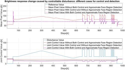
Figure 14. Fixed ROI where the outer tiles (red) are not included in the ROI (green tiles).

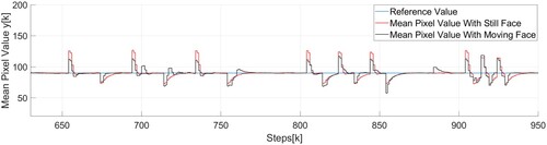
In Figure 15, a similar experiment was conducted in which the comparison between scenarios with still and moving face is made. Similar to the previous figure, The higher subplot shows the reference value and the calculated mean pixel values, while the lower subplot contains the disturbance value and the joint control values. Although smaller peaks and valleys are shown as a result of the region boundaries change, the algorithm performs well in both cases. If the graph is slightly enlarged in the upper subplot Figure 16, it is seen that the reference value was reached in 10–15 frames, which translates to 330–495 milliseconds.

Figure 15. Brightness response change caused by controllable disturbance with control and region detection with still and moving face.

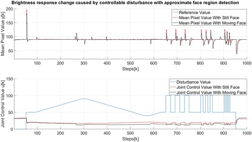
Figure 16. Enlarged brightness response change caused by controllable disturbance with control and region detection with still and moving face.

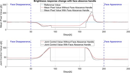
The control algorithm with approximate face region detection works similarly to the control algorithm with a fixed region when the face is present. The biggest difference occurs when the face goes outside the scene or ROI. In a control system with a fixed region, the joint control value reaches its peak without getting close to the mean pixel value which wears the equipment faster. As seen in Figure 17, if the approximate face region detection and face absence handle are employed, the joint control value is set to a low value after the face disappears, but high enough to recognize the face region when the face reappears. Regarding the execution time of the automatic brightness control with the approximate face region detection, the average execution time of the approximate face region detection, automatic brightness control, and changing parameters is 9.13 milliseconds.

Figure 17. Face absence behavior without and with face absence handle.

5. Discussion

Automatic brightness control with approximate face region detection in real-time is a complex system that stretches over the image and signal processing, control systems, and embedded system optimization. Regarding the approximate face region detection, although the face region detection variants outperform some segments, the Viola-Jones algorithm as the most common embedded face detection algorithm produces better results overall. This is somewhat expected because the Viola-Jones algorithm is face-oriented, while the approximate face region detection is sampled region-oriented. While this degrades the detection quality, the execution time is greatly improved, which is the main asset of the algorithm. Also, the region detected with the proposed method changes less frequently than the region from the Viola-Jones algorithm, which is beneficial for the automatic brightness control system. Moreover, the proposed method doesn't have face region detection problems with different face poses and glasses. Regarding the approximate face region detection experiment, the best result is acquired when the temporal step is added to variant A with only hysteresis active, and the time series median filtering can be omitted to further reduce the execution time. The performance drop can be seen in the daytime when the background can also be bright at some parts, which confuses the algorithm and misinterprets those parts for a foreground. The reflectance of the clothes is also a factor that can deteriorate the approximate face region detection. In that case, multiple thresholds can determine multiple brightness classes. To improve the behavior of the face region detection algorithm, the voting system between the variants of the algorithm can be implemented to make it more robust. If the detected regions exist in more than one variant, it is considered part of the face region. The second approach is the width and height face region ratio in which not all vertical rectangles are candidates for the face region, but only the ones that satisfy the criteria of the expected face region ratios between the width and the height. While this also reduces the execution time, it can interfere with the region expansion if the case of a subject wearing bright clothes. The approaches will be tested in the next experiments. Face tracking algorithms are often used in similar solutions. While the accuracy would increase by using the additional face tracking methods, the complexity of the algorithm would also increase, and, with it, the hardware demands and the execution time. The temporal step of the approximate face region detection behaves similarly to a face tracking algorithm by including the previous region values in the calculation of the current boundaries. Another solution to increase performance is a convolutional neural network. Although it is stated in [19] that the convolutional neural networks are not practical for real-time face detection, a lightweight and optimized neural network can be used for fast face detection, but in that case, a large dataset is needed for training the classifier. The FADID dataset, as stated before, is small and lacks sudden ambient light changes and significant face occlusion, such as a hand covering the face. The other impacts, such as the distance effect of the face to camera were not measured, however, the effect is simulated through an experiment with the results in Figure 13. As the face approaches the camera, the regions in which the face is located are getting brighter, which is equivalent to increasing the disturbance value with the NIR light source. Also, when the face is moving from the camera, the brightness decreases, which is also represented by the falling ramp in Figure 13. Creating a new dataset is an option, but that includes implementing the system in a vehicle to obtain the fast light changes which can then be achieved by driving towards, from, and by sunlight, through tunnels during the day, along tree lines, and towards car lights at night. The temporal step of the approximate face detection algorithm can also be added to the other face detection algorithms. Regarding the automatic brightness control, it is seen that the optimal brightness control converges fast to the target value, which is an improvement in comparison to [15, 16], and also to the previous work [5] by adding approximate face region detection. However, it is hard to make direct comparisons to other methods because most of the implementations are aimed at different applications and implemented on different systems, as stated in [4]. The main task of the system is to control the face brightness to have the best input image to the face analysis algorithms, however, the automatic brightness control with face detection is not so widely covered and there aren't many papers to compare with. While the results are quite similar between the scenarios with and without approximate face region detection, the biggest difference occurs when the face is absent from a scene. In that case, the mean pixel value drops significantly and the system struggles to achieve the reference value. The joint control value u can be high and, when the face returns, the image is too bright to detect the face. For that reason, the face absence handle described earlier is necessary. Regarding the split-range feedback controller, it was determined that the D term can be omitted and analog gain was held fixed because it often caused oscillations around the reference value. The algorithm performs quite fast (9.13 ms) which leaves room for the mentioned improvements, even a denser grid for mean pixel value matrix calculation if the embedded system can provide it.

6. Conclusion

In this paper, the improved fast automatic brightness control algorithm with approximate spatio-temporal approximate face region detection optimized for the embedded systems is proposed. The algorithm finds the face region and adjusts the region brightness rapidly to prepare the input frame for face analysis. The automatic brightness control is based on a split-range PID feedback controller with a face absence handle, while the approximate face detection is based on sampled skin detection. To the best of the authors' knowledge, little work has been done in infrared automatic brightness control with approximate face region detection, while the face absence handle is first introduced in this paper. The algorithm performs well with fast convergence and little to no oscillations in normal operating mode. The proposed method outperforms the state-of-the-art solutions in automatic face brightness control. It is an easily implementable and resourceful solution best suited for a real-world application with hardware and space limitations, such as the automotive industry, as shown in the FADID dataset. In future work, the face region detection improvements will be tested such as the voting system, region width/height ratios, and multiple thresholds. Also, the system will be tested in real-life conditions to check the overall system performance to get the proper feedback and information about the needed future improvements.

Disclosure statement

No potential conflict of interest was reported by the author(s).

Additional information

Funding

This work was supported by European Fund for Regional Development [System for detection of driver fatigue and distraction].

References

- Su Y, Kuo CCJ. Fast and robust camera's auto exposure control using convex or concave model. In: 2015 IEEE International Conference on Consumer Electronics (ICCE). Las Vegas (NV): IEEE; 2015. p. 13–14.
- Ali S, Jonmohamadi Y, Takeda Y, et al. Supervised scene illumination control in stereo arthroscopes for robot assisted minimally invasive surgery. IEEE Sens J. 2020;21(10):11577–11587.
- Tomasi J, Wagstaff B, Waslander SL, et al. Learned camera gain and exposure control for improved visual feature detection and matching. IEEE Robotics Autom Lett. 2021;6(2):2028–2035.
- Sousa RM, Wäny M, Santos P, et al. Automatic illumination control for an endoscopy sensor. Microprocess Microsyst. 2020;72:102920.
- Vugrin J, Lončarić S. Automatic brightness control for face analysis in near-infrared spectrum. In: 2021 International Conference on Signal Processing and Machine Learning (CONF-SPML). Stanford (CA): IEEE; 2021. p. 296–299.
- Viola P, Jones M. Rapid object detection using a boosted cascade of simple features. In: Proceedings of the 2001 IEEE Computer Society Conference on Computer Vision and Pattern Recognition. CVPR 2001. Vol. 1. Kauai (HI): IEEE; 2001. p. I–I.
- Laurie J, Higgins N, Peynot T, et al. Dedicated exposure control for remote photoplethysmography. IEEE Access. 2020;8:116642–116652.
- King DE. Dlib-ml: a machine learning toolkit. J Machine Learning Res. 2009;10:1755–1758.
- Wu C, Samadani R, Gunawardane P. Same frame rate ir to enhance visible video conference lighting. In: 2011 18th IEEE International Conference on Image Processing. Brussels: IEEE; 2011. p. 1521–1524.
- Ebisawa Y. Realtime 3D position detection of human pupil. In: 2004 IEEE Symposium on Virtual Environments, Human-Computer Interfaces and Measurement Systems (VCIMS). Boston (MA): IEEE; 2004. p. 8–12.
- Di W, Wang R, Ge P, et al. Driver eye feature extraction based on infrared illuminator. In: 2009 IEEE Intelligent Vehicles Symposium. Xi'an: IEEE; 2009. p. 330–334.
- Otsu N. A threshold selection method from gray-level histograms. IEEE Trans Syst Man Cybern. 1979;9(1):62–66.
- Jeong M, Kwak J, Ko BC, et al. Facial landmark detection based on an ensemble of local weighted regressors during real driving situation. In: 2016 23rd International Conference on Pattern Recognition (ICPR). Cancun: IEEE; 2016. p. 2198–2203.
- Wu F, You W, Smith JS, et al. Image-image translation to enhance near infrared face recognition. In: 2019 IEEE International Conference on Image Processing (ICIP). Taipei: IEEE; 2019. p. 3442–3446.
- Dowdall J, Pavlidis I, Bebis G. Face detection in the near-ir spectrum. Image Vis Comput. 2003;21(7):565–578.
- Gnatyuk V, Zavalishin S, Petrova X, et al. Fast automatic exposure adjustment method for iris recognition system. In: 2019 11th International Conference on Electronics, Computers and Artificial Intelligence (ECAI). Pitesti: IEEE; 2019. p. 1–6.
- Jeong M, Ko BC, Kwak S, et al. Driver facial landmark detection in real driving situations. IEEE Trans Circuits Syst Video Technol. 2018;28(10):2753–2767.
- Dai T, Dou Y, Tian H, et al. The study of classifier detection time based on opencv. In: 2012 Fifth International Symposium on Computational Intelligence and Design, Vol. 2. Hangzhou: IEEE; 2012. p. 466–469.
- Tomita Y, Suzuki S, Fukai H, et al. The classification system with the evolutionary computation. In: 2010 11th IEEE International Workshop on Advanced Motion Control (AMC). Nagaoka: IEEE; 2010. p. 750–755.