
 ?Mathematical formulae have been encoded as MathML and are displayed in this HTML version using MathJax in order to improve their display. Uncheck the box to turn MathJax off. This feature requires Javascript. Click on a formula to zoom.
Abstract
Medical image analysis presents a significant problem in the field of image registration. Recently, medical image registration has been recognized as a helpful tool for medical professionals. Current state-of-the-art approaches solely focus on source image registration and lack quantitative measurement for object deviation in terms of loosening, subsidence and anteversion related to surgery. In this article, we have provided motion vectors for recognizing the object deviation, in addition to detecting and selecting the feature points. Firstly, the feature points will be detected using Hessian matrix determinants and octave and level sampling. Then the strongest feature points are selected which will be utilized for identifying the object deviation with respect to the reference image through motion vectors. The objective of this work is to combine image registration and temporal differencing to achieve independent motion detection. In comparison to state-of-the-art approaches, the proposed methodology achieves higher Information Ratio (IR), Mutual Information Ratio (MIR) and their lower bounds for image registration.
1. Introduction
The term “image registration” refers to the method through which several data sets are transformed into a single coordinate system. Several images taken from different sensors, at various periods, depths, distances, and/or vantage points may constitute data. Registration is required for comparing or integrating data from these different measurements. Due to the vast range of applications to which image registration is applied and various types of degradations in source images, it is impossible to create a universal approach that is suited for all applications. Image registration methods should consider not only the assumed type of geometric deformation between source images, but also noise corruption, desired registration accuracy, radiometric deformations, and the properties of the data that are specific to the targeted application.
Image registration has numerous applications, including but not limited to automatic target recognition in the military [Citation1], medical imaging, computer vision, and the collection and analysis of satellite imagery [Citation2]. Image registration is a pre-processing step in all fusion techniques [Citation3–6] where multiple modalities of registered images will be combined into a single image, object detection [Citation7], object recognition [Citation8,Citation9], and image classification [Citation10–12].
Medical image registration involves matching of feature points in images of the same patient recorded at different times (multitemporal analysis) for more accurate diagnosis, prognosis, treatment, and follow-up [Citation13]. Clinical applications requiring spatial alignment of anatomical features such as monitoring tumour growth and healing therapy, treatment verification, and comparison of the patient’s data with anatomical atlases, make registration an indispensable part of medical image processing. Image registration is useful when multiple imaging modalities are being utilized to record anatomical body structure such as Magnetic Resonance Spectroscopy (MRS). Positron Emission Tomography (PET), Magnetic Resonance Imaging (MRI) [Citation14], Computed Tomography (CT) [Citation15], Single Photon Emission Computed Tomography (SPECT), Ultrasound (US).
To discuss the utilization of research advances into practice and to provide a fair standard across competing approaches, the Learn2Reg [Citation16] evaluates intra- and inter-patient, mono- and multimodal medical image registration for 3D images. This evaluation covers a broad spectrum of anatomies (brain, abdomen, and thorax), modalities (ultrasound, CT, MR), and availability of annotations
In 2D/3D registration, the notions of two weighted histograms of gradient directions and second-order spatial histograms were introduced and their benefits and drawbacks were assessed [Citation17]. The gradient-weighted histogram is responsive to transformations in rotation and scaling but not translation. It causes a complex registration procedure and restricts the algorithm to a narrow convergence range for translation parameters. For statistical feature extraction, the approach relies on a spatially weighted histogram of gradient directions.
An exhaustive survey of applications of Transformers to medical image processing, including segmentation, detection, classification, restoration, synthesis, registration, and the generation of clinical reports was done in [Citation18]. The authors have created a taxonomy for each of these uses, pinpointed the unique difficulties of each with suggestions for how to overcome them, and brought attention to the most current developments in each area.
In [Citation19], the featured surface matching method was shown to be effective for registering lung images. To deform and align a 3D volume image with a 3D surface image, the technique was applied to volume-to-surface deformable image registration. The surface feature is extracted by calculating the curvature variation, and the correspondence between two surface points is established using the matching scheme.
To perform 2D/3D femur registration, [Citation20] suggests using the core decompression technique as a surgical example, with the goal of registering preoperative MRI with intraoperative 2D fluoroscopic images. The registration's ensuing transformation is then utilized to generate overlays of preoperative MRI annotations and planning data for use by surgeons as a type of visual guidance.
There are some hurdles during the registration process, namely low resolution of images [Citation21,Citation22], deformation, organ motion, identification of motion vectors for detecting object deviation from source images, images with different modalities and the noise of interventional images [Citation23]. Motivated by the above limitations and the demand for faster algorithms we proposed a novel method for image registration in this paper, that not only registers but also finds the amount of deviation using motion vectors. In this article we have taken datasets involving hip replacement diagnosis, brain, retina, and other human body scans where image registration plays an important role. After surgery and during follow-up visits, the doctor should be able to determine with certainty whether or not the replaced metal in the hip inserted through surgery is in the correct position even years later. In this scenario, our proposed method aids medical professionals. Similar object detection was done for retinal and brain scans.
2. Related work
Feature detection plays a crucial part in image processing. In order to compare identical objects in two images, one of which may be misaligned, feature detection is helpful. Many methods for processing medical images [Citation24] rely on feature detection, which entails extracting the features of a certain image automatically based on the object's unique content. The method described above was employed in a wide variety of computer vision applications [Citation25–28]. Examples of computer vision include object recognition and object tracing, which involve registering the feature points of an image.
In this section, we formulated how differential operators can be used as feature points and first-order convolutional filters to calculate Hessain determinants which in turn are used to find feature points.
2.1. Differential operators for feature points
If an image is focused using transformations like shifting with some scale or otherwise rotating at a certain angle, then it is feasible for object identification in an image. The following three stages are commonly used to determine the correspondence between the pixels in an image, while there are many others that can be utilized. The first stage is interest points selection from various locations like corners, globules, and intersections in an image. The second stage involves determining the feature vector from the surrounding pixels of each point of interest under various observational scenarios [Citation29]. The last stage involves calculating the motion vectors by comparing the feature vectors from the two source images. In order to execute this kind of matching, the distance between the vectors must be determined. The correspondence between pixels can be determined with the help of standard geometrical transformations like the Euclidean distance.
2.2. Convolutional filters
One of the simplest linear filters in the spatial domain is the box filter. It replaces a pixel in an image with its average value of neighbourhood pixels [Citation30], and this is a simple average method performed on pixels. Box filters are used to find the average value of neighbourhood 4-connectivity or 8- connectivity pixels.
Convolutional filters working with masks of size 3*3 or 9*9 sometimes are called convolution-symmetric kernels [Citation31]. Let the coordinates of the image be (x,y) and “L” be the scale parameter which can characterize the size of the filter. The general property of the convolutional filter is given in Equation (1).
(1)
(1) where
represents an image in spatial domain,
is a mask of size 3*3 used in our proposed method,
denotes spatial coordinates.
Discrete differential operators are used in convolutional filters with several scales which are used to improve the filter efficiency and perform parameterized operation with the suitable kernel by above-mentioned variable “L”. To do this operation, first-order and second-order convolutional filters can be used.
2.2.1. First-order convolutional filter
Let us consider a digital image “u” and this can be operated with the true values of the operator at a scale accomplished with prime coordinate referred to as “D” multiplied with
. It creates the convolutional filter with a suitable size given by Equation (2).
(2)
(2)
Recollecting the information where the symbol [.] represents the round-off operation to the next higher value of integer. The first-order convolutional filter operator is given by Equation (3).
(3)
(3) where
and
are responses of first-order filter.
These filters use first-order partial derivatives as operators in a preference scale ℓ. We can get a good suitable formula for its impulse of “D” multiplied with operator.
(4)
(4)
Computational complexity calculation using the integrated image as explained in Equation (2) we can pre-determine the integrated image say “U”, seven consecutive additions are enough to evaluate those operators irrespective of size of the parameter ℓ. Now let us consider and evaluate [Citation32] the same Equation (2) with “b” and “a” equal to ℓ and c = -ℓ, d = −1.
We can get, the final filter coefficients using Equation (5),
(5)
(5)
3. Proposed method for medical image registration
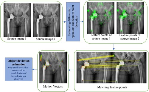
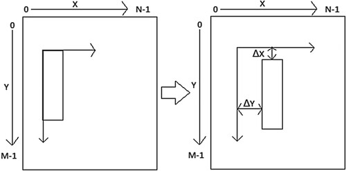
The proposed image registration process attempts to discover matching feature points between two images and spatially align them. There are five major steps as depicted in Figure , that the proposed method has to go through for image registration. These could be listed as follows:
Step 1: Estimating differential operators for the source images.
Step 2: Feature points detection.
Step 3: Feature points selection.
Step 4: Feature points matching.
Step 5: Object deviation estimation through motion vectors
Figure 1. Schematic of proposed method.
Each step is explained in detail in the following sub-sections.
3.1. Estimating differential operators for the source images
Let the two source images be and
. Differential operators will be calculated separately for each source image by using a convolutional filter Equation (3).
3.2. Feature points detection
In Section 2, the structures of first-order convolutional filters and how these filters are configured with their parameters were explained. In this section, feature points through multi-scale adaptive local feature detection are found. Convolutional filter [Citation33] produces the response with scale-invariant property, i.e. the filter response should not vary with its operator’s scale. The term “multi-scale” is introduced here because, for multi-modal source images, multi-scale feature point detection can be employed.
Feature detection follows the steps shown below in Algorithm 1. Here, the inputs are and
and it produces a list of feature points from the source images.
Algorithm 1 for detecting feature points
Step-1: Initialization of two differential operators and
Step-2: For loop starts with L = 1 to 2
Calculate Hessian matrix
End For loop
Step-3: Select feature points
Step-4: For loop starts here to perform Octave Sampling
For loop starts here to perform Level Sampling
Calculate
List feature points by adding to Hessian matrix coefficients
End for loop
End for loop
Step-5: Return all feature points
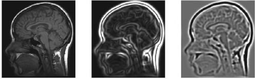
In Algorithm 1, indicates level sampling, we can detect feature points and some important terms related to this algorithm like Hessian matrix coefficients, and active samplers as explained below. Second-order partial derivatives are arranged in a square matrix, which forms a Hessian matrix. Usually, the Hessian matrix uses the functional determinants. An example of a Hessian matrix applied on an MRI image is shown in Figure . For the leftmost image of Figure [Citation34] when the Hessian operator is applied, the edges will smoothen as in a centre image of Figure . Further smoothening of the image can be obtained as shown in the rightmost image by increasing the order of the Hessian operator.
Figure 2. An example of Hessian matrix applied on MRI image.
Hessian determinant calculation using convolution filters: The scale-independent Hessian matrix determinants, can be calculated from Equation (6).
(6)
(6) where
and
are calculated from Equation (3). As we mentioned in Algorithm 1, scaling can be achieved from the relation
and here the constant predefined weight “w” is 0.912. Normalization factors are required to get the scale invariance property, generally, we will take
as a normalization factor. While calculating the Hessian determinant, the numerical tolerance will come into the picture to overcome this weighting factor “w” which was used.
3.3. Feature points selection
After detecting the feature points, we have to select only a few of them which are adaptively considered matched with the reference image. This can be achieved by considering the neighbourhood pixels. In this selection, the class of transformation which we used at the time of the feature detection procedure was important. By considering similarity parameters like location and shape, scale estimation is jointly performed with similarity transformation.
In this methodology, the common interest or desirable points are considered as the local maxima of the determinants of the Hessian matrix of an image
. Now, the detection of maxima is performed [Citation30] by considering P, Q, and R neighbourhood pixels, generally P = Q = R = 3, and comparing the box space with the nearest neighbourhood pixels. The above-said procedure is given in Algorithm 2. This algorithm consists of input arguments that are maxima of the determinants of the Hessian matrix
of an image
, octave sampling
, Level of interest
,
values at “
” and “
”. The output arguments are a list of key points.
Algorithm 2 for key points selection
Step-1: initialization of octave sampler, level of interest and hessian determinants
Step-2: Calculate
Step-3: For loop start with 0 to M-1
Perform Correspondence.
For loop start with 0 to N-1
Perform Correspondence.
Use Equation (7) to fix the threshold
Maximum dominance calculation for
Interpolation parameters Calculation for
End for loop
End for loop
Step-4: Return the list of key points
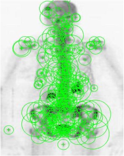
Procedure to set the threshold: Thresholding is an essential process after quantization with octaves. Here we use four octaves and two levels for analysis so that we can analyse 8 scales of representation. Using the method as in [Citation35], it is not only a computationally efficient method of image representation but also provides noise immunity. We can get the key features by applying a threshold on Hessian determinants .
(7)
(7) We have to remember that this operator is scale-invariant and is constant. This normalization can be achieved using simple mathematical operations. By using the trial and error method too, we can set the threshold [Citation36], let the threshold value be 103 and the reference image interval be [0,255]. Figure describes setting the points of interest with reference to Hessian determinants
after the thresholding operation. The radii of the green circles are variable, in this application, the radii are set to 2.5 times the L (Box Scale).
Figure 3. Illustration of interest point detection.
3.4. Matching the key points
After selecting the feature points from two images, and
match the feature points which are represented by their point of interest
with their corresponding descriptors
. We know that, for this type of descriptor, the interest points must satisfy the condition X ε [−1,1]64 which indicates a vector with dimension 64 and its Euclidean norm is
. The comparison between the interest points was performed using Euclidean distance since these interest points are considered as vectors. Using a thresholding technique called Nearest-Neighbour Distance Ratio (NNDR), we can combine the features. Here, we calculate the Euclidean distance by comparing the descriptor
with the image
and
.
(8)
(8)
Let us consider one-megapixel image, almost millions of scalar products are computed from the second image “”, this extends the computational complexity. Therefore, to lessen the computational complexity in the matching procedure, we need to compare the Laplacian [Citation37] signs of key features. If the two descriptor’s signs are not equal, then those are considered as unlikely similar. In this case, there is no need to compare the key features and the comparison is discarded.
To match the key points, we need to find the most important and reliable correspondence from several number of reputed features, this leads to the best match of features. In the other way, if we consider the similarity distance only into account, it is necessary to separate the true match from the false match. The nearest neighbour matching method may or may not produce the best match because it considers only correspondence between
and its most similar one, denoted by
where
is given in Equation (9),
(9)
(9)
The Nearest Neighbour Distance Threshold is a proximity search technique which is used in pattern recognition, computer vision, etc., this is a straightforward method to find the correspondence by fixing the threshold on the similarity measure. Indeed, such a method of matching produces a negotiation between false positive numbers and false negative numbers. Therefore, instead of using this type of thresholding method [Citation38], we used the Nearest Neighbour Distance ratio, which is a simple and reliable statistical method to discard mismatches.
In this method of matching, we need to find the ratio of the first and second nearest neighbour pixels and measure the correspondence between them. For doing this, first, we have to compute Yℓ1 from the desired Xk, such that
(10)
(10)
Finally, compare the corresponding ratio to a suitable threshold “t” and follow the condition, if , then the correspondence was confirmed in this decision, and the threshold was set to t = 0.8, we may increase or decrease the threshold using trial and error methods. We are dealing with medical images hence the threshold was set to maximum value. After matching is complete, it is necessary to find the deviation of the matched points. This is explained in the below section motion vector calculation.
3.5. Motion vectors calculation
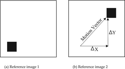
The motion estimation theory between two consecutive images using features is described in this section. The key idea of motion estimation is to determine [Citation39] the displacement between two successive frames as shown in Figure .
Figure 4. Displacement between frames: (a) Reference image 1 and (b) Reference image 2.
In the simplest form, the problem can be described by Equation (11). This equation only permits the registration of translational movement in x and y and the intensity levels are expected to be the same all over the image.
(11)
(11)
Frame Translation: The general model of inconsistency between two objects in two respective frames is translation. Translation can identify the movement of any particular region in an image. Naturally, if an image is affected by translational movement, then it indicates objects [Citation40] in the foreground have been moved. Suppose the translational movement is outside the reference image, then the new frame is created by the combination of both old coordinates plus translation coefficients.
(12)
(12) where
and
are the old coordinates of the image in which the translation operation was performed,
and
are the new coordinates after performing the translation operation. The numerical values
and
are the small translational movement in X-axis and Y-axis direction, respectively.
Each pixel of the frame was translated and new coordinates were obtained from Equation (12). The entire frame was updated with new coordinates and the frame was neither damaged nor corrupted by noise. In the translation operation [Citation41], all pixels of the original image are imposed in the output image, and the region of interest is moved to the desired position [Citation38,Citation42] using Equation (12). If all pixels of the original image are left unchanged, then the translated image is the same as the original image which means that there is no change in the output image. We can observe a slight difference between moving the pixel region and translating the pixel region if the original pixel region was filled with homogenous grey levels. An example of a translation operation is given in Figure .
Figure 5. Example for translational operation.
Since the pixel values of an image are integers, the translation procedure is straight forward and if we use sub-pixel values, we may use the bilinear interpolation method.
Rotation of an image: Spatial transformation techniques have a vital role in many image processing applications like CT, and MRI images. Rotational operation is one of the linear spatial transformation methods [Citation43]. This type of operation depends on the direction of rotation and rotational angle.
Let us consider the camera movement to be an anti-clockwise rotation. Then the entire frame will be a clockwise rotation of all pixel values to a new location computed using Equation (13).
(13)
(13) where θ represents the rotational angle. For more reliable analysis, Equation (14) is written where the quantity
measures the average value.
(14)
(14)
Equation (14) is rewritten as in Equation (15),
(15)
(15)
In numerous cases and more desirable cases involving medical applications [Citation44], analysing the rotational movement of individual objects in the frame is needed. Equation (13) enables such type of mechanism. As mentioned in the above equations, we conclude the new coordinates for the rotated image will be as given in Equation (16).
(16)
(16)
4. Results and discussion
4.1. Experiment setup
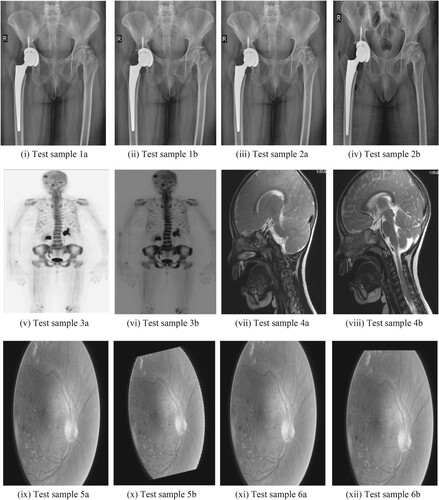
Subjective and objective evaluations have validated the performance analysis of the proposed medical image registration using octave and level sampling. The simulation is run on a computer equipped with a 12th Gen Intel(R) Core(TM) i7-12700H processor, a RAM size of 16GB, and an NVIDIA GEFORCE RTX GPU. Figure presents a total of 10 test samples [Citation45–47] to be considered to evaluate the proposed method. The proposed medical image registration using octave and level sampling is compared with four state-of-the art methods: Scale Invariant Optical Flow [Citation48] (SIOF), Constrained Least Squares [Citation49] (CLS), Cost Function Minimization [Citation50] (CFM), and Coherent Pixel Correspondence [Citation51] (CPC). We have used the default values that the authors of these existing methods have provided. For quantitative analysis, we have used four quality metrics [Citation52,Citation53]: Information Ratio (QIR), Lower bound Information Ratio (QLIR), Mutual Information Ratio (QMIR), and Lower bound Mutual Information Ratio (QLMIR).
Figure 6. Ten medical test samples used for registration: (i) Test sample 1a (ii) Test sample 1b (iii) Test sample 2a (iv) Test sample 2b (v) Test sample 3a (vi) Test sample 3b (vii) Test sample 4a (viii) Test sample 4b (ix) Test sample 5a (x) Test sample 5b (xi) Test sample 6a (xii) Test sample 6b (xiii) Test sample 7a (xiv) Test sample 7b (xv) Test sample 8a (xvi) Test sample 8b (xvii) Test sample 9a (xviii) Test sample 9b (xix) Test sample 10a (xx) Test sample 10b.
4.2. Quality metrics
In this section, we used quantitative methods to analyse the effectiveness of the proposed algorithm. An image is described through a matrix of dimension where each element is referred to as a pixel. Each pixel is itself a vector in
, where D is the colour depth of an image and each dimension represents grey scale intensity.
We assume that a set of images
is drawn from the distribution
where
. In the following, we refer to each
as a frame. For a given
,
let
be the 2-D vector corresponding to the colour
; we refer to
as the component image of the colour
or the
channel of the image
. Finally,
for
the pixel
for the grey level
at frame
4.2.1. Information ratio (QIR)
Using Equation (17), can be calculated as the self-information of an image intensity relative to the information content of individual pixels with the same intensity.
(17)
(17) where
,
is self-information of the
level estimation as
4.2.2. Mutual information ratio (QMIR)
Equation (18) is used to calculate QMIR which is analogous to that of the QIR, but in terms of a pair of intensity values over two images.
(18)
(18)
4.2.3. Lower bound information ratio (QLIR)
Equation (19) gives the value of QLIR as a function of entropy and mutual information. The computational difficulty of calculating the feature count is greatly reduced by using this approximation.
(19)
(19) where
is entropy.
4.2.4. Lower bound mutual information ratio (QLMIR)
QLMIR gives useful bounds between the entropy and the IR, and between the mutual information and the MIR. A lower bound on is calculated as a function of
as shown in Equation (20).
(20)
(20) where
is mutual information.
4.3. Results
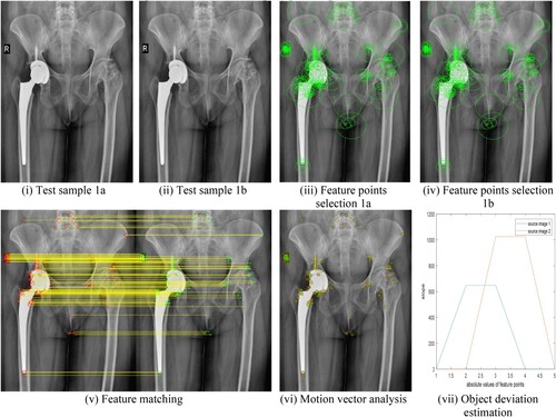
In this section, we used ten test samples of medical images. The experiment with the proposed method of image registration not only performed feature detection but also identified how much the position of artificial bone inserted during surgery deviated from the reference image after surgery and during follow-ups. Figure (i) is a reference image of bone immediately after surgery and Figure (ii) is the image taken during follow-up visits say after a few months of surgery. From Equation (7), the strongest key points are selected as shown in Figure (iii) and (iv). Here we can identify clearly that there was no deviation in the bone position, hence as seen in Figure (vi) no motion vectors exist. The same statement can be justified by the quantitative values of Figure (vii). Two polygons are shown in Figure (vii) for two reference images Figure (i) and (ii) have no slope which indicates that there is no deviation. In Figure (v) slope of the matched features is zero. The motion vector analysis performed on the test sample further justifies the proposed algorithm.
Figure 7. (i–vii) Hip replacement surgery without bone position deviation: (i) Test sample 1a (ii) Test sample 1b (iii) Feature points selection 1a (iv) Feature points selection 1b (v) Feature matching (vi) Motion vector analysis (vii) Object deviation estimation.
Consider Figure (i) which shows a reference image of bone immediately after surgery and Figure (ii) is the image taken during follow-up visits say after a few months of surgery. From Equation (7), the strongest key points are selected as shown in Figure (iii) and (iv). As it can be observed clearly in Figure (v) there exists a slope for each of the features matched, which indicates there is a mismatch in bone position between images of Figure (i) and (ii), hence motion vectors exist in Figure (vi). Two polygons shown in Figure (vii) for two reference images Figure (i) and (ii) have a slope which indicates that there is some deviation. If we compare Figure (vi) and Figure (vi), in the former there are no motion vectors because there is no deviation, but in the latter, we can observe a few motion vectors. This way we have three ways of identifying deviation namely feature matching, motion vector and polygon slope.
Figure 8. (i–vii) Hip replacement surgery with bone position deviation: (i) Test sample 2a (ii) Test sample 2b (iii) Feature points selection 2a (iv) Feature points selection 2b (v) Feature matching (vi) Motion vector analysis (vii) Object deviation estimation.
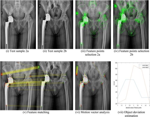
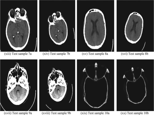
Our algorithm was tested not only on hip replacement surgery but also on other medical applications involving the retina, brain and a few other body scans. Similar analysis as in Figure and Figure was made for test samples Figure (v) to (xx) whose quantitative analysis is given in Figure and Table . The proposed algorithm also identifies the amount of deviation like very small deviation/ no deviation/ small deviation/ high deviation as discussed in Figure . During the MATLAB simulation of the test samples in 1a and 1b of Figure , “no deviation” was observed while test samples 2a and 2b of Figure showed “high deviation”.
Figure 9. Objective assessment of different image registration methods including proposed method: (i) Information Ratio, QIR (ii) Lower bound Information Ratio, QLIR (iii) Mutual Information Ratio, QMIR (iv) Lower bound Mutual Information Ratio, QLMIR.
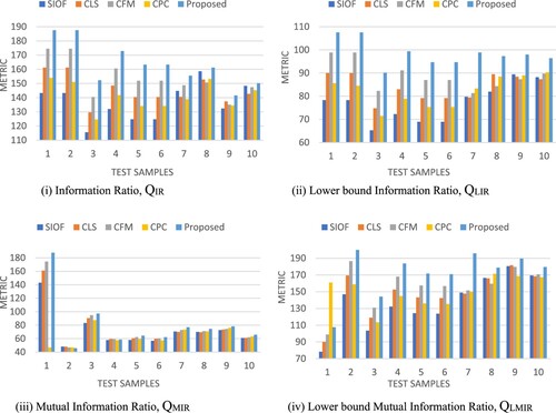
Table 1. Registration metrics.
For quantitative analysis of the image registration methods, Information Ratio (QIR) and Mutual Information Ratio (QMIR) [Citation54] are used. Here QIR and QMIR will be calculated including their lower bounds, i.e. QLIR and QLMIR are the functions of mutual information and entropy. These metrics are useful to minimize the computational complexity in identifying the feature count. These metrics will be useful to evaluate the registered image from the perspective of common features count that can be identified among given samples. The metrics for the ten test samples of medical images are given in Table .
To visualize the registration effect of the four existing and our proposed medical image registration techniques, we offered a graphical representation of objective assessment indices in Figure . In every metric, the proposed algorithm has obtained superior outcomes than the state-of-the-art approaches.
Figure presents the average objective performance analysis of medical image registration methods. When compared to the four state-of-the-art approaches, our proposed method outperforms them all.
Figure 10. Average metric values of proposed and existing techniques.
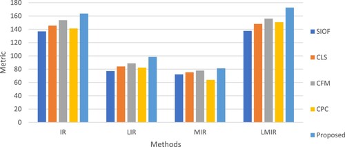
Whether using subjective visual evaluation or objective indicators, the suggested strategy yields improved overall registration outcomes. Nevertheless, we may state that the proposed method produces satisfactory results.
5. Conclusion and future scope
Medical image registration with object deviation estimation through motion vectors using octave and level sampling has been proposed in this article. Many medical registration algorithms have the limitation of quantitative analysis while detecting abnormalities like loosening, subsidence and anteversion. The proposed algorithm will perform quantitative analysis in terms of Information Ratio (QIR), Mutual Information Ratio (QMIR) and their lower bounds. Our algorithm helps medical practitioners detect the amount of object deviation post-surgery using motion vector analysis. Both qualitative and quantitative assessments have found that our method outperforms the current state of art methods. In the proposed method, we concentrated on translational movement only. There is a possibility to identify the abnormalities even if it is affected by rotational and skew motion. This will be possible through 3-D image analysis.
Disclosure statement
No potential conflict of interest was reported by the author(s).
Data availability statement
Any data and code used in this paper are available from the authors upon reasonable request.
References
- Vasu GT, Palanisamy P. Visible and infrared image fusion using distributed anisotropic guided filter. Sens Imaging. 2023;24(40):1–17. doi:10.1007/s11220-023-00447-0
- Fiza S, Safinaz S. Multi-focus image fusion using edge discriminative diffusion filter for satellite images. Multimed Tools Appl. 2024:1–20. doi:10.1007/s11042-024-18174-3
- Tirumala Vasu G, Palanisamy P. Gradient-based multi-focus image fusion using foreground and background pattern recognition with weighted anisotropic diffusion filter. Signal Image Video Process. 2023;17(5):2531–2543. doi:10.1007/s11760-022-02470-2
- Tirumala Vasu G, Palanisamy P. CT and MRI multi-modal medical image fusion using weight-optimized anisotropic diffusion filtering. Soft Comput. 2023;27(13):9105–9117. doi:10.1007/s00500-023-08419-y
- Tirumala Vasu G, Palanisamy P. Multi-focus image fusion using anisotropic diffusion filter. Soft Comput. 2022;26(24):14029–14040. doi:10.1007/s00500-022-07562-2
- Fiza S, SS. Multi-sensor medical image fusion using computational harmonic analysis with wave atoms. India Patent 27192, 17-3-2023.
- Potter PD, Kypraios I, Steven Verstockt CP, et al. Automatic passengers counting In public rail transport using wavelets. Automatika. 2012;53(4):321–334. doi:10.7305/automatika.53-4.227
- Gökçe B, Sonugür G. Recognition of dynamic objects from UGVs using interconnected neural network-based computer vision system. Automatika. 2022;63(2):244–258. doi:10.1080/00051144.2022.2031539
- Gunasekaran K, Raja J, Pitchai R. Deep multimodal biometric recognition using contourlet derivative weighted rank fusion with human face, fingerprint and iris images. Automatika. 2019;60(3):253–265. doi:10.1080/00051144.2019.1565681
- Vasu GT, Fiza S, Tatekalva S, et al. Deep learning model based object detection and image classification. Solid State Technol. 2018;61(3):15–25.
- Vasu GT, Fiza S, Kubra A, et al. Deep learning model based early plant disease detection. NeuroQuantology. 2022;20(20):1818–1824.
- Fiza S, Vasu GT, Kubra A, et al. Machine learning algorithms based subclinical keratoconus detection. NeuroQuantology. 2022;20(20):1825–1837.
- Goshtasby AA. Theory and applications of image registration. John Wiley & Sons; 2017. Online ISBN: 9781119171744, doi:10.1002/9781119171744
- Duana L, Yuanb G, Gongc L, et al. Adversarial learning for deformable registration of brain MR image using a multi-scale fully convolutional network. Biomed Signal Process Control. 2019;53:101562, doi:10.1016/j.bspc.2019.101562
- Cao Z, Dong E, Zheng Q, et al. Accurate inverse-consistent symmetric optical flow for 4D CT lung registration. Biomed Signal Process Control. 2016;24:25–33. doi:10.1016/j.bspc.2015.09.005
- Hering A, Hansen L, Mok TCW, et al. Learn2Reg: comprehensive multi-task medical image registration challenge, dataset and evaluation in the era of deep learning. IEEE Trans Med Imaging. 2023;42(3):697–712. doi:10.1109/TMI.2022.3213983
- Ban Y, Wang Y, Liu S, et al. 2D/3D multimode medical image alignment based on spatial histograms. Applied Sciences. 2022;12(16):8261. doi:10.3390/app12168261
- Shamshad F, Khan S, Zamir SW, et al. Transformers in medical imaging: a survey. Med Image Anal. 2023;88:102802, doi:10.1016/j.media.2023.102802
- Su S-T, Ho M-C, Yen J-Y, et al. Lung image registration by featured surface matching method. Comput Method Biomech Biomed Eng Imaging Visual. 2022;10(6):653–662. doi:10.1080/21681163.2021.2019614
- Ku P-C, Martin-Gomez A, Gao C, et al. Towards 2D/3D registration of the preoperative MRI to intraoperative fluoroscopic images for visualisation of bone defects. Comput Method Biomech Biomed Eng Imaging Visual. 2023;11(4):1096–1105. doi:10.1080/21681163.2022.2152375
- Zheng W, Yang B, Xiao Y, et al. Low-dose CT image post-processing based on learn-type sparse transform. Sensors. 2022;22(8):2883, doi:10.3390/s22082883
- Lu S, Yang B, Xiao Y, et al. Iterative reconstruction of low-dose CT based on differential sparse. Biomed Signal Process Control. 2023;79(2):104204, doi:10.1016/j.bspc.2022.104204
- Hajnal JV, Hill DLG. Medical image registration. CRC Press; 2001. doi:10.1201/9781420042474
- Akinyelu AA, Zaccagna F, Grist JT, et al. Brain tumor diagnosis using machine learning, convolutional neural networks, capsule neural networks and vision transformers, applied to MRI: a survey. J Imaging. 2022;8(8). doi:10.3390/jimaging8080205
- Sokooti H, Yousefi S, Elmahdy MS, et al. Hierarchical prediction of registration misalignment using a convolutional LSTM: application to chest CT scans. IEEE Access. 2021;9:62008–62020. doi:10.1109/ACCESS.2021.3074124
- Begum N, Badshah N, Ibrahim M, et al. On two algorithms for multi-modality image registration based on Gaussian curvature and application to medical images. IEEE Access. 2021;9:10586–10603. doi:10.1109/ACCESS.2021.3050651
- Zhang T, Zhao R, Chen Z. Application of migration image registration algorithm based on improved SURF in remote sensing image mosaic. IEEE Access. 2020;8:163637–163645. doi:10.1109/ACCESS.2020.3020808
- Zhao E, Li L, Song M, et al. Research on image registration algorithm and its application in photovoltaic images. IEEE J Photovol. 2020;10(2):595–606. doi:10.1109/JPHOTOV.2019.2958149
- Zang X, Zhao W, Toth J, et al. Multimodal registration for image-guided EBUS bronchoscopy. J Imaging. 2022;8(7):189, doi:10.3390/jimaging8070189
- Varga D. No-Reference quality assessment of authentically distorted images based on local and global features. J Imaging. 2022;8(6):173, doi:10.3390/jimaging8060173
- Lee S-S, Jang S-J, Kim J, et al. Memory-efficient SURF architecture for ASIC. Electron Lett. 2014;50(15):1058–1059. doi:10.1049/el.2013.4102
- Yu X, Ding R, Shao J, et al. Hyperspectral remote sensing image feature representation method based on CAE-H with nuclear norm constraint. Electronics (Basel). 2021;10(21): 1–13. doi:10.1049/el.2013.4102
- Kawazoe Y, Shimamoto K, Yamaguchi R, et al. Faster R-CNN-based glomerular detection in multistained human whole slide images. J Imaging. 2018;4(7):91, doi:10.3390/jimaging4070091
- Hladůvka J, König A, Gröller E. Exploiting eigenvalues of the hessian matrix for volume decimation. WSCG(2001). 2001.
- Li Y, Yang C, Zhang L, et al. A novel SURF based on a unified model of appearance and motion-variation. IEEE Access. 2018;6:31065–31076. doi:10.1109/ACCESS.2018.2832290
- Jardim S, António J, Mora C. Graphical image region extraction with K-means clustering and watershed. J. Imaging. 2022;8(6):163, doi:10.3390/jimaging8060163
- Leng C, Zhang H. The prediction of eigenvalues of the normalized laplacian matrix for image registration). 2016 12th International Conference on Natural Computation, Fuzzy Systems and Knowledge Discovery (ICNC-FSKD). 2016: 1620–1624. doi:10.1109/FSKD.2016.7603419
- Balakrishnan G, Zhao A, Sabuncu MR, et al. Voxelmorph: a learning framework for deformable medical image registration. IEEE Trans Med Imaging. 2019;38(8):1788–1800. doi:10.1109/TMI.2019.2897538
- Hou B, Khanal B, Alansary A, et al. 3-D reconstruction in canonical Co-ordinate space from arbitrarily oriented 2-D images. IEEE Trans Med Imaging. 2018;37(8):1737–1750. doi:10.1109/TMI.2018.2798801
- Kumar Reddy Yelampalli P, Nayak J, Gaidhane VH. Daubechies wavelet-based local feature descriptor for multimodal medical image registration. IET Image Proc. 2018;12(10):1692–1702. doi:10.1049/iet-ipr.2017.1305
- Do VL, Yun KY. A low-power VLSI architecture for full-search block-matching motion estimation. IEEE Trans Circuits Syst Video Technol. 1998;8(4):393–398. doi:10.1109/76.709406
- Su JK, Mersereau RM. Motion estimation methods for overlapped block motion compensation. IEEE Trans Image Process. 2000;9(9):1509–1521. doi:10.1109/83.862628
- Yeo H, Hu YH. A novel matching criterion and low power architecture for real-time block based motion estimation. Proceedings of International Conference on Application Specific Systems, Architectures and Processors: ASAP ‘96, 1996.
- Matsushita Y, Ofek E, Ge W, et al. Full-frame video stabilization with motion inpainting. IEEE Trans Pattern Anal Mach Intell. 2006;28(7):1150–1163. doi:10.1109/TPAMI.2006.141
- Ding L, Kang T, Kuriyan A, et al. Flori21: fluorescein angiography longitudinal retinal image registration dataset. IEEE Dataport. November 2021.
- Rahman T, Chowdhury M, Khandakar A, et al. Aseptic loose hip implant x-ray database. [Data set] Kaggle. 2022.
- Johnson KA, Becker JA. “Atlas, the whole brain.” [Online]. Available: https://www.med.harvard.edu/aanlib/.
- Yu Q, Jiang Y, Zhao W, et al. High-Precision pixelwise SAR–optical image registration via flow fusion estimation based on an attention mechanism. IEEE J. Sel. Top. Appl. Earth Obs. Remote Sens. 2022;15:3958–3971. doi:10.1109/JSTARS.2022.3172449
- Pallotta L, Giunta G, Clemente C. Sar image registration in the presence of rotation and translation: a constrained least squares approach. IEEE Geosci Remote Sens Lett. 2021;18(9):1595–1599. doi:10.1109/LGRS.2020.3005198
- Abuzneid M, Mahmood A. Image registration based on a minimized cost function and SURF algorithm. International Conference Image Analysis and Recognition. 2017.
- Quidu I, Myers V, Midtgaard Ø, et al. Subpixel image registration for coherent change detection between two high resolution sonar passes. International Conference on Underwater Remote Sensing (ICoURS); Brest, France, 2012.
- Mirabadi AK, Rini S. The information & mutual information ratio for counting image features and their matches. 2020 Iran Workshop on Communication and Information Theory; Tehran, Iran, 2020.
- Hu L, Gao L, Li Y, et al. Feature-specific mutual information variation for multi-label feature selection. Inf Sci (Ny). 2022;593:449–471. doi:10.1016/j.ins.2022.02.024
- Khajegili Mirabadi A, Rini S. The information & mutual information ratio for counting image features and their matches. 2020 Iran Workshop on Communication and Information Theory (IWCIT), 2020.