SwinVNETR: Swin V-net Transformer with non-local block for volumetric MRI Brain Tumor Segmentation

Abstract

Brain Tumor Segmentation (BTS) and classification are important and growing research fields. Magnetic resonance imaging (MRI) is commonly used in the diagnosis of brain tumours owing to its low radiation exposure and high image quality. One of the current subjects in the field of medical imaging is how to quickly and precisely segment MRI scans of brain tumours. Unfortunately, most existing brain tumour segmentation algorithms use inadequate 2D picture segmentation methods and fail to capture the spatial correlation between features. In this study, we propose a segmentation model (SwinVNETR) Swin V-NetTRansformer-based architecture with a non-local block. This model was trained using the Brain Tumor Segmentation Challenge BraTS 2021 dataset. The Dice similarity coefficients for the enhanced tumour (ET), whole tumour (WT), and tumour core (TC) are 0.84, 0.91, and 0.87, respectively. By leveraging this methodology, we can segment brain tumours more accurately than ever before. In conclusion, we present the findings of our model through the application of the Grad-CAM methodology, an eXplainable Artificial Intelligence (XAI) technique utilized to elucidate the insights derived from the model, which helped in better understanding; doctors can better diagnose and treat patients with brain tumours.

KEYWORDS:

• Deep learning
• Swin Transformer
• brain tumour segmentation
• non-local block
• explainable AI
• Grad-CAM

1. Introduction

According to information from Cancer Research UK, there are more than 130 diverse types of brain tumours. These tumours can initiate in any part of the brain or spinal cord and are commonly named after the type of cells from which they originate. Glioblastoma multiforme (GBM) is the most prevalent and aggressive primary brain tumour in adults [1]. Brain tumours encompass both benign and malignant variants. The noteworthy types highlighted in the research findings include the following: 1. Glioblastoma Multiforme (GBM): Recognized as the most common and aggressive primary brain tumour in adults [1]. 2. Gliomas: Gliomas emerge as a prevalent type of adult brain tumour, constituting 78 percent of malignant brain tumours. Originating from glial cells, they encompass subtypes such as astrocytomas, oligodendrogliomas, and ependymomas [2]. 3. Meningiomas: Typically benign, these tumours develop from the meninges, which are thin layers of tissue covering the brain and spinal cord [3]. 4. Pituitary Tumors: Situated in the pituitary gland at the base of the brain, these tumours are largely non-cancerous [3]. 5. Chordomas, Chondrosarcoma, and Medulloblastoma: Examples of rare and specific brain tumours, each characterized by distinct features and treatment implications [3]. It is crucial to emphasize that the segmentation and classification of brain tumours hinges on diverse factors, including the cell type involved, tumour location, and behaviour (benign or malignant). The specific type of brain tumour significantly shapes the chosen treatment approach and profoundly influences patient prognosis. Brain tumour segmentation is an important area of research for medical professionals. This involves the use of advanced technology to accurately identify and segment brain tumours and classify them into different types. Researchers are constantly striving to find the most effective methods for brain tumour segmentation to provide better treatment options for patients. Spatial coding and reconstruction technology is at the heart of nuclear MRI, one of the most widely used medical imaging methods for identifying and treating brain illnesses [4]. The brain tumour segmentation process requires considerable time and effort, and it is possible for mistakes to be made or diagnoses to go unnoticed when doctors manually segment brain tumours from MRI images. Although MRI offers several benefits in the supplemental diagnosis of illnesses, it has drawbacks [5]. Image segmentation plays a crucial role in the diagnosis and treatment of glioma. For instance, surgical planning, postoperative monitoring, and survival rate can benefit from an accurate glioma segmentation mask [6].

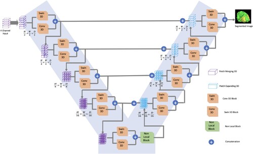
Recent studies in the fields of computer vision and pattern recognition have shed light on the ability of convolutional neural networks (CNNs) to address challenging problems such as classification, segmentation, and object recognition while achieving the most advanced performance levels. The success of CNN can be attributed in part to its capability to learn a hierarchical representation of unlabelled input data without the need for specially specified features. The level of abstraction of the generated features is said to increase as the inputs are processed via various levels of the network. Deeper layers utilize filters with significantly wider receptive fields, which allow them to capture global information, whereas shallower layers only capture information relevant to their immediate surroundings [7]. Nevertheless, most segmentation algorithms use 2D images, which are incapable of obtaining the spatial dependence between features. To solve the aforementioned issue, we propose a method based on a spatial and channel Swin V-Net TRansformer-based architecture with a non-local block. Figure 1 shows the SwinVNETR structure used in this study.

Figure 1. Overall architecture of Swin VNETR.

Explainable Artificial Intelligence (XAI) is an emerging field dedicated to enhancing the interpretability and transparency of machine-learning models. Among the prominent methods within XAI is Guided GradCAM, a fusion of Gradient-weighted Class Activation Mapping (Grad-CAM) and Gradient Boosting (GBP), which is designed to produce precise attributions [8]. Grad-CAM itself serves as a visualization technique that offers interpretability by pinpointing the crucial features in the input image. In this article, we delve into the concepts of XAI and Grad-CAM, and explore their applications across various domains.

The significance of XAI is growing as AI systems play an increasingly prominent role in diverse sectors, such as healthcare, finance, and transportation. Understanding the decision-making processes of AI models is imperative to ensuring their reliability and trustworthiness. Grad-CAM, a popular XAI method, generates heat maps by amalgamating gradient information from the final convolutional layer of a deep neural network [8]. These heatmaps offer insights into the regions of the input image that contribute significantly to the model's decision-making, thereby providing a valuable understanding of the model’s behaviour. After training with the SwinVNETR model, the results were explained using the Grad-CAM.

2. Related work

2.1. Traditional machine learning methods

Utilizing super-pixel-wise feature extraction techniques, the classical Support Vector Machine model was applied to the segmentation of brain tumours. However, this technique can also be applied to 2D images. The 2013 Brats dataset yielded only binary results [9].

2.2. Deep learning-based methodology

Deep-learning algorithms have proven to be highly effective in stabilizing training and uncovering hierarchical features, resulting in enhanced segmentation accuracy. Consequently, deep learning algorithms have emerged as a rapid and efficient methodology for analyzing medical images, providing substantial advancements over conventional approaches [10]. Unlike traditional GAN-based segmentation methods, this study’s Softmax probability maps were indirectly optimized. Specifically, this method combines softmax probability maps into a single segmentation image to arrive at the result. The authors utilized the Brats 2015 dataset but used GAN's lack of interpretability to understand the segmentation [11].

A Cascade Convolutional Neural Network (C-CNN) model augmented with a Distance-Wise Attention (DWA) mechanism has emerged as a notable advancement in brain tumour segmentation research. By leveraging the BRATS 2018 dataset, this model addresses the complexity of the task by incorporating multimodal MRI images containing various histological subregions. The C-CNN architecture offers a cascade approach, enabling the gradual refinement of segmentation boundaries, whereas the DWA mechanism enhances accuracy by focusing on the spatial relationships between distant voxels [12]. The CNN-based brain tumour segmentation algorithm stands out for its high-performance metrics. This approach employs the N4ITK method for bias field distortion correction in MRI, ensuring that the preprocessing steps enhance the image quality and consistency. Additionally, the implementation of dropout and batch normalization techniques contributes to more efficient training and improved model generalization, reducing the risk of overfitting and enhancing the robustness of the segmentation results [13].

Numerous segmentation techniques are available for brain tumours, such as threshold-based methods, conventional machine learning, region growing, clustering algorithms, and deep learning [14]. In this study, we focus on a deep-learning methodology for brain tumour segmentation. Deep learning-based segmentation of brain tumours has demonstrated promising performance in the precise identification of brain tumour regions. For brain tumour segmentation, deep neural networks (DNN), three-dimensional unified networks (3-D U-Net deep), and fully convolutional networks (FCN) are only a few of the many deep-learning methods developed by researchers. 3D convolutional neural networks for tumour segmentation extract long-range contextual information from adjacent 3D medical image slices using 2D convolutional layers [15]. This context is then provided to a 3D CNN that analyzes the current slice in conjunction with the context of adjacent slices. Using a long-range 2D context, this method reduces the number of parameters required by the 3D CNN, allowing it to process larger volumes of medical data with fewer computational resources. The results of using the CNN method in the BRATS 2017 challenge for multiclass segmentation of malignant brain tumours. The CNN method yielded accurate segmentations with median Dice scores achieved whole tumour 0.918, tumour core 0.883, and enhancing tumour 0.854. However, the problem with this method is that the long-range 2D context can capture contextual information from adjacent segments; it may not be sufficient to capture the complete context of the tumour, particularly when the tumour extends across multiple slices. This may lead to less-precise segmentation results. The 3D Fusion Transformer model employs a multihead self-attention mechanism (MHSA), where each attention head is computed independently, posing challenges in integrating structures between layers [16].

A significant number of researchers in the BraTS 2016 challenge used a 3D U-net, which led to impressive segmentation accuracy across the board and in the tumour core. When trained on the BraTS 2015 training dataset (with 60% of the data utilized for training and 40% for testing), they reported Dice scores of 0.89, 0.76, and 0.37 for the whole tumour, tumour core, and active tumour, respectively. The high cost of computing is a drawback of Unet design [17]. The 3D Attention-based U-Net paper proposes a methodology that consolidates three non-native MRI volumes into a unified stacked multimodal volume, enhancing the spatial information in the input and enabling one-time segmentation. The addition of an attention mechanism to the decoder side of the U-Net de-emphasizes healthy tissues and highlights malignant tissues, leading to improved generalization power and reduced computational resource requirements. This study used the BraTS2021 dataset [18]. This study introduced an innovative architecture built on a 3D U-Net model. This design incorporates multiple skip connections by employing cost-efficient pre-trained 3D MobileNetV2 blocks and attention modules. The incorporation of these elements contributes to maintaining manageable model size and expediting convergence. To enhance the feature exchange, the authors introduced extra skip connections between the encoder and decoder blocks, maximizing the utilization of extracted features throughout the segmentation process. Additionally, attention modules play a crucial role in filtering out irrelevant features transmitted through skip connections, preserving computational resources, while simultaneously enhancing accuracy [19].

The fusion of CNN and Transformer components for segmentation is highlighted, particularly focusing on the integration of DConv, Swin Transformer Encoder, and Decoder. This approach incorporates multiscale attention mechanisms within the CNN framework to enhance comprehension of spatial relationships and contextual information. A detailed description of these components reveals their synergistic role in effectively capturing both the local and global features. Additionally, the proposal of CSU-Net, an encoder-decoder architecture, leverages this hybrid integration to achieve superior segmentation performance, demonstrating its potential for accurately delineating complex structures within medical imaging tasks [20].

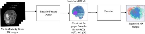
Existing brain tumour segmentation methods have several significant drawbacks. These methods rely on handcrafted features, which often fail to capture the complex and varied appearances of brain tumours, resulting in limited feature representation. Additionally, many classical methods operate independently on 2D slices of MRI scans, leading to inconsistencies across slices and failure to exploit the 3D spatial context of the brain and tumour. This slice-by-slice analysis often necessitates significant manual tuning and intervention, such as setting thresholds or selecting regions of interest, making the process time consuming and susceptible to user bias. Classical methods are also sensitive to noise, intensity inhomogeneities, and artifacts in MRI images, and require extensive preprocessing to mitigate these issues. Furthermore, these methods do not generalize well across different datasets or imaging protocols, often necessitating re-optimization or re-training for each new dataset. Integrating multiple MRI modalities (such as T1, T2, and FLAIR) into classical methods poses a challenge, typically requiring complex fusion strategies that may not be optimal. SwinVNETR is a revolutionary method that we proposed. Brain tumours can be segmented using a Swin V-net Transformer equipped with a Non-local Block. In step 1, the 3D MRI data are sent to the encoder, where features are extracted using 3D Swin and 3D convolutional neural networks. In step 2, a Non-local Block is employed to assemble data on long-range dependencies from the encoder part. In Step 3, the encoder's output features are forwarded to the decoder, where they are up-sampled. In Step 4, the concluding layer of the SwinVNETR model serves as the input for 3D Gradient-weighted Class Activation Mapping (Grad-CAM) to provide explainability. This process involves visualizing the gradient information to understand how the model makes predictions.

3. Proposed methodology

3.1. Swin V-Net transformer model

Recent advances in computer vision technology have led to the increased use of CNN for medical image analysis, employing deep learning methods. Although CNN excels in processing 2D images, some therapeutically relevant medical data are only available in 3D. Therefore, in this study, 3D MRI images of brain tumours were segmented using V-Net. To accomplish comprehensive semantic segmentation of 3D medical images, V-Net is an enhanced version of a Fully Convolutional neural network) FCN’s 3D network architecture by replacing the whole connection layer with a convolution layer. Specifically, we propose combining a 3D Swin Vision transformer (swin ViT) with a CNN encoder and decoder.

Figure 1 shows the left and right halves of the network. The encoding path, located on the left side of the network, employs convolution to automatically extract relevant picture features from the MRI scans. It included a swin transformer to improve the picture recognition capacity and decrease the resolution after each layer by a predetermined amount. The non-local block is inserted as a final step in the encoding process to learn distant feature locations. More information about the Swin Transformer and non-local block is provided below. The decoding path, located on the right side of the network, was responsible for recreating the full feature map. In the last stage of the network, the segmentation results were classified using SoftMax into three groups: enhanced tumour (ET), whole tumour (WT), and tumour core (TC).

3.2. Swin 3D

Swin Block3D was inspired by the block module of the Swin Transformer [21]. The construction of the Swin Block3D is shown in Figure 2a. It consists of two main sections, each consisting of two parts. The first part uses a LayerNorm (LN) layer, the second part uses an MLP module, and the third part uses a shifted-window multi-head self-attention3D (SW_MSA_3D) module. In contrast to the W_MSA_3D module used in the first part, the SW_MSA_3D module was implemented in the second part. The following equation can be used to calculate Swin Block3D: (1) $\begin{array}{rl}{X}^{t_1}& =L{N}_1(X^{L-1})+W\mathrm{\_SA\_}3D(L{N}_1(X^{L-1}))\end{array}$(1) (2) $\begin{array}{rl}{X}^t& =L{N}_2(X^{t_1})+\mathrm{MLP}(L{N}_2(X^{t_1}))\end{array}$(2) (3) $\begin{array}{rl}{X}^{t_2}& =L{N}_3(X^t)+\mathrm{SW}\mathrm{\_MSA\_}3D(L{N}_3(X^t))\end{array}$(3) (4) $\begin{array}{rl}{X}^L& =L{N}_4(X^{t_2})+\mathrm{MLP}(L{N}_4(X^{t_2}))\end{array}$(4)

Figure 2. (a). Swin 3D blocks included W-MSA-3D and MLP, (b). 3D convolutional block.

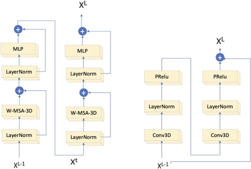
The calculation of Swin Block3D can be summarized by equations (1), (2), (3), and (4). The given formula utilizes only temporary variables Xt1 and Xt2. Before calculating the self-attention, the Swin Block3D Self Attention module transforms the feature maps into voxel patches and then transforms each voxel patch into a one-dimensional token. After the self-awareness calculation is complete, the tokens are transformed back into their respective voxel patches and added to the feature map. The dimensional transformation of the matrix maps the token regions to the voxel regions. A voxel patch in space [h, w, d] can be represented by a token of length h × w × d, and a token in space [h, w, d] can be transformed into a token in space [h, w, d] by using a matrix. We utilized the Rearrange class found in the einops library to facilitate the transformation of the tokens and feature maps.

3.3. 3D convolution block

As shown in Figure 2b, the 3D Conv Block module uses a double-layered configuration of 1 × 1 × 1 convolutional layers, LayerNorm layers, and PRelu layers to learn local picture dependencies. The logic behind the calculations in this component is as follows: (5) $\begin{array}{rl}{X}^t& =\mathrm{PReLu}1(L{N}_1(\mathrm{Conv}3D_1(X)))\end{array}$(5) (6) $\begin{array}{rl}{X}^t& =\mathrm{PReLu}(\mathrm{LN}(\mathrm{Conv}3D(X^t)))\end{array}$(6) (7) $\begin{array}{rl}Y& =X^t\times X\end{array}$(7)

In these equations, X represents the input to Conv Block3D, Y represents the output, and X^t is a variable used throughout the conversion process. To reduce the computational load of this module, we used depth-wise separable convolution instead of regular convolution. This sub-module employs the VAN implementation to perform feature convergence of X^L and X through multiplication, rather than addition, to better match the fine-grained information in the image.

3.4. Non-local block

In the domain of 3D MRI brain tumour segmentation, the implementation of a Non-local block presents several enhancements in the segmentation process. This mechanism allows the model to encompass information from the entire input volume, transcending a narrow focus on the local regions. Given the intricate and diverse patterns exhibited by tumours in 3D MRI segmentation, which can extend across substantial spatial distances, this global perspective is crucial. It contributes to the capacity of the model to grasp long-range dependencies by considering the interactions between all positions in the input space. This augmentation is particularly beneficial for improving the model's discernment of intricate structures associated with brain tumours. Furthermore, the incorporation of a Non-local block facilitates a superior generalization [27]. This was achieved by empowering the model to learn the intricate relationships between various spatial positions across a diverse range of examples in the training dataset. Given the significant variability in tumour shapes and sizes among different patients, the non-local block has emerged as a valuable tool for mitigating the sensitivity of the segmentation process to spatial variations. By considering relationships and dependencies across all positions in the 3D volume, this mechanism ensures a more robust and adaptable approach to brain tumour segmentation. The non-local block is based on [22], who coined the term “non-local neural networks”. The interference with the classical self-attention mechanism is not local in nature. The structure of the non-local block is illustrated in Figure 3. However, non-local blocks are especially helpful for picture classification and segmentation, which require the capture of long-range relationships. The Non-local block equation is expressed as follows: (8) $\begin{array}{rl}{Y}_i& =\frac{1}{C(X)}\sum _{\mathrm{\forall }j}f(X_i,X_j)g(X_j)\end{array}$(8) (9) $\begin{array}{rl}{Z}_i& =Y_{i}W+b\end{array}$(9)

Figure 3. Structure of non-local block.

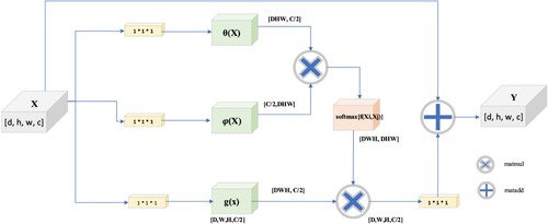
In this context, “X” represents a feature-mapped input signal, and “i” represents a position index that can be in space, time, or both. The value that “j” returns is calculated by considering every possible outcome. The binary function “f” determines the similarity relationship between “i” and all “j”, whereas the unary function “g(x)” is utilized to calculate the representation of the input signal at location “j.” According to [22], the response is calculated by adding all the response factors, or C(x).

This section is defined in accordance with [22], $C(X)=\sum \mathrm{\forall jf}(X_i,X_j)$. Consequently, the non-local evaluation of the equation is $y_i=\text{softmax}[f(X_i,X_j)]g(X_j)$. According to the theory of computer vision, this behaviour is consistent with the self-attention relation. There is hardly any difference in self-attention performance between the abstract forms g(x) and (Xi, Xj). To keep things straightforward, we performed linear processing on X using a convolution kernel of size 1 × 1 × 1. The equation used for computing is as follows: (10) $\begin{array}{rl}g(x)& =\mathrm{xW}+b\end{array}$(10) (11) $\begin{array}{rl}f(X_i,X_j)& =\theta (X_i)\phi (X_j{)}^T\end{array}$(11) (12) $\begin{array}{rl}\theta (X)& =X{W}_{\theta }^T+b_{\theta }\end{array}$(12) (13) $\begin{array}{rl}\phi (X)& =X{W}_{\phi }^T+b_{\phi }\end{array}$(13)

Assuming a feature map as the input signal x to a non-local block is crucial for our method. The D, W, H, and C values of the feature map refer to the depth, width, height, and channels, respectively. Before doing anything further to X, we split the channel count of the input feature map in half and use it as the number of convolutional kernels. Therefore, it is necessary to have channels for counting C/2, θ(X), φ(X), and g(X) at fixed dimensions is required. in a predetermined number of dimensions. The goal is to reduce the amount of computation required while maintaining the performance of the non-local block unaffected. Multiplying the θ(X) and φ(X) matrices by [dwh, C/2] and [C/2, Y] respectively enables the non-local self-attention method. Multiplying the result by g(X) yields [DWH, C/2], which undergoes morphological transformation. The input feature map is convolved with C convolution kernels of size 1 × 1 × 1, where C is the total number of convolution kernels. Although both complete connection layers and non-local layers must calculate the entire feature map to extract the necessary features, non-local layers offer more benefits for accurate feature extraction. When the size of the non-local output is the same as the size of the original feature map, the entire connection layer must transform the non-local output into a list of neurons with a fixed number, size, and loss of some location information.

The proposed method integrates a Swin Vision Transformer with a CNN encoder and decoder to process 3D MRI images of brain tumours. The encoder extracts relevant features from the multimodal 3D MRI images, the nonlocal block captures long-range dependencies, and the decoder reconstructs the feature map, as shown in Figure 4. The Swin Block3D and 3D Conv Block modules enhance the ability of the model to process fine-grained information and capture detailed contextual relationships. The non-local block provides a global perspective, which is crucial for accurately segmenting complex tumour structures. This integrated approach results in superior segmentation performance, as demonstrated by the high Dice similarity coefficients for enhanced tumour (ET), whole tumour (WT), and tumour core (TC) segmentation.

Figure 4. Flow diagram for proposed model execution.

4. Dataset

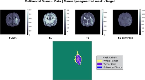
The purpose of this work was to construct a Swin V-Net transformer using the BraTS 2021 MRI dataset. Pre-processed 3D images (in NifTi file format) were included. There were 8,000 MRIs in this data collection, representing 2,000 unique patients. The multiparametric MRI scans of the BraTS 2021 project are distinguished by native (T1) and post-contrast (T1Gd) T1-weighted (T1Gd) volumes, T2-weighted (T2) and T2-FLAIR volumes, and segmentation ground-truth data [23]. Each volume was scanned using standard techniques and equipment of the acquiring institution. The size of the input image was 240 × 240 × 155 pixels, as shown in Figure 5. The data were compiled from a wide variety of sources using several distinct MRI scanners. The enhanced tumour, whole tumour, and tumour core are labelled in the annotations. The complete tumour, its core, and its augmentation were all covered by combined annotations. We used the BraTS 2021 dataset, which contained 1251 training instances and 219 validation cases, to fine-tune our models. Evaluation Metrics:

Figure 5. BraTs2021 native (T1) and post-contrast (T1Gd) T1-weighted (T1Gd) volumes, T2-weighted (T2) and T2-FLAIR volumes 3D MRI Images.

5. Implementation

The first step involves masked volume inpainting, which fills in missing or corrupted regions within medical images, thereby ensuring a comprehensive representation of tumour volumes. Subsequently, 3D contrastive coding enhances the visualization and differentiation of tumour tissues from normal brain tissues by encoding the contrast information. Following this, the rotation prediction predicts the optimal orientation of the brain tumour for further analysis and treatment planning. Deep learning algorithms further contributed by extracting features and classifying tissue types, facilitated by the AdamW optimizer with a warm-up cosine schedule of 500 iterations. The initial learning rate was 4e-4, momentum was 0.9, and decay was 1e-5 for 450,000 iterations. Leveraging NVIDIA Tesla P100 GPUs accelerates these computationally intensive tasks, expedites analysis, and enables quicker clinical decisions. The model was implemented using Python packages, such as PyTorch, SimpleITK, and Nibabel. Pseudo-code for the proposed model is provided below.

Table

Pseudo-code for Proposed Model
1  input_dimensions = (batch_size, channels, height, width, depth) # Input shape for 3D MRI scans
2  num_classes = 3 # Number of classes: ET, WT, TC
3  def encoder(x):
4    x = ConvBlock(x, filters = [64, 128, 256]) # filter sizes
5    # Add Swin Transformer layers here
6    swin_layers = []
7    for _ in range(num_swin_layers):
8        swin_layer = SwinTransformerLayer(embedding_dim, num_heads, window_size)
9      swin_layers.append(swin_layer)
10   for i, swin_layer in enumerate(swin_layers):
11      res_block = ResidualConnection(swin_layer(x))
12      x = DownSampling(res_block, stride = stride)
12   # Non-Local Block
13    x = NonLocalBlock(x)
14   return x
15  def decoder(features, skip_connections):
16      upsampled_features = UpSampling(features)
17      x = concatenate([upsampled_features, skip_connections])
18      x = ConvBlock(x, filters = [256, 128, 64])
19      x = ConcatenateFeatures() # Combine multiple levels of features
20      x = ConvBlock(x, filters = [64, num_classes])
21      x = SoftmaxActivation(axis = −1)
22      return x
23  def BrainTumorSegmentationNetwork():
24      input_layer = Input(shape = input_dimensions)
25      encoded_features = encoder(input_layer)
26      skip_connections = []
27      for _ in range(len(encoder.__dict__[‘__globals__’][‘swin_layers’])):
28        skip_connection = UpSampling(encoded_features)
29        skip_connections.append(skip_connection)
30        encoded_features = encoded_features + skip_connection
31    segmentation_output = decoder(encoded_features, skip_connections)
32    model = Model(inputs = input_layer, outputs = segmentation_output)
33    compile_model(model, optimizer = 'adamW’, loss = 'binary_crossentropy’)
34    return model

6. Evaluation metrics

The Dice coefficient is the primary target of the loss function in our model. The Dice coefficient is a function used to measure similarity, and its values range from zero to one [28–42]. The equation that characterizes this relationship is as follows: (14) $\begin{array}{r}\text{Dice}\text{Coefficient = }\frac{2||X\cap Y||}{||X||+||Y||}=\frac{2\mathrm{TP}}{2\mathrm{TP}+\mathrm{FP}+\mathrm{FN}}\end{array}$(14) where X represents the model predictions, Y represents the actual data, TP represents the tumour voxels that were correctly recognized, FN represents the non-tumour voxels that were correctly identified, and FP represents the non-tumour voxels that were mislabelled as tumours by the model. The Dice coefficient ranges from 0 to 1 and indicates the accuracy with which a model predicts an outcome. The Dice coefficients are closer to 1 when the forecasts are closer to the GT.

The Hausdorff distance (HD) [24] serves as a measure of the spatial discrepancy between the surface vertices of two binary masks. Its formal definition is as follows: (15) $\begin{array}{r}\text{HD}(\mathbf{G}\text{,}\mathbf{R})=\max \left\{\underset{s_{\mathbf{G}}}{\sup }d(s_{\mathbf{G}},S(\mathbf{R})),\underset{s_{\mathbf{R}}}{\sup }d(s_{\mathbf{R}},S(\mathbf{G}))\right\}\end{array}$(15) Here, S_R and S_G denote the surface vertices of the automated segmentation result R and the corresponding ground truth segmentation G, respectively. The symbol sup represents the supremum. To ensure resilience against potential noise-induced issues arising from small segmentations, a robust modification of the HD metric is introduced, termed H95, which utilizes the 95th percentile instead of the maximum distance.

In the evaluation of brain tumour segmentation tasks, performance was assessed using both the Dice Similarity Coefficient (DSC) and the H95 metric. These metrics were computed for distinct tumour subregions, such as the Whole Tumor (WT), Tumor Core (TC), and Enhancing Tumor (ET). This evaluation methodology remained consistent with the practices established in prior studies.

7. Results and discussion

Our models generated mean Dice coefficients of 0.838 for enhanced tumours, 0.871 for tumour cores, and 0.905 for whole tumours on the Brats2021 validation dataset and Hausdorff distance for the different tumours (Table 1). Figure 6 displays the segmented findings obtained with the help of the ITK-SNAP tool In the comparison presented in Table 1, various models underwent evaluation on the BRATS 2021 validation dataset for brain tumour segmentation, revealing distinctive performance characteristics and trade-offs. The assessed models, which encompassed 3D U-Net, V-Net, UnetR, TransBTS, SwinBTS, AttentionUnet, Swin Pure Unet3D, and SwinVNETR, demonstrated variations in both parameter size and segmentation accuracy across the ET, TC, and WT subregions. Notably, SwinVNETR exhibited commendable segmentation accuracy across all subregions, achieving a high Mean Dice score. This comparative analysis sheds light on the diverse performance aspects of these models, emphasizing the need for careful consideration of both the parameter efficiency and segmentation precision. The notable performance of SwinVNETR underscores its effectiveness in accurately delineating brain tumour subregions. These insights serve as valuable resources for researchers and practitioners seeking to make informed decisions regarding model selection based on their specific requirements. Ongoing advancements in medical image segmentation can benefit from these findings, with the aim of improving the accuracy, efficiency, and applicability in clinical contexts. In Figure 7. Panel A shows input FLAIR images. Panel B presents the ground-truth segmentation for comparison. Panel C illustrates the feature extraction process within a Non-Local block. Finally, Panel D displays the segmented results, highlighting the Whole Tumor (WT), Tumor Core (TC), and Enhancing Tumor (ET). In Figure 8, the presented graph illustrates the variability in Dice coefficients, serving as a valuable tool for assessing the efficacy of the model in adapting to the validation dataset from Brats2021. The curves in the graph represent the Dice coefficients for three distinct channels: ET (Enhancing Tumor), TC (Tumor Core), and WT (Whole Tumor). The Dice coefficient, a commonly used metric in image segmentation tasks, measures the extent of overlap between the predicted and ground-truth segmentation masks. Consequently, this graph offers insights into the performance of the model across different tumour regions during the validation phase, providing a comprehensive perspective on its segmentation accuracy for the specified channels.

Figure 6. A) Brain image with tumour, B) Whole Tumor highlighted in green, C) Enhanced Tumor in yellow, D) Tumor Core in red, visualized using ITK-SNAP [25] software tool used to view the brain tumour segmentation.

Figure 7. A. an Flair image as an input B. the ground truth of the validation data C. the feature extraction process during the Non-Local block D. the final segmented WT, TC, and ET.

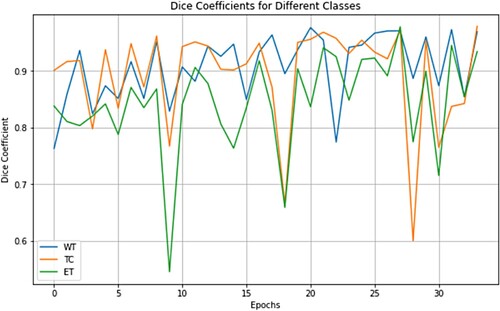
Figure 8. Curves illustrating the variation in Dice coefficients were used to assess the model's fitting capability on the validation dataset of Brats2021. These curves depict the Dice coefficients for the ET, TC, and WT channels.

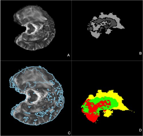
Table 1. Comparison table of brats 2021 validation dataset.

		Mean Dice			Hausdorff distance
Name of the model	Params Size	ET	TC	WT	ET	TC	WT
3D U-Net	15.834	0.825	0.844	0.900	3.71	7.36	4.82
V-Net	182.432	0.815	0.840	0.751	2.88	6.17	6.43
UnetR	204.899	0.842	0.853	0.905	3.12	8.46	4.59
TransBTS	65.975	0.824	0.843	0.889	3.89	5.54	4.22
SwinBTS	71.394	0.828	0.843	0.896	4.02	5.16	4.68
AttentionUnet	47.257	0.841	0.851	0.870	3.57	6.83	4.06
Swin Pure Unet3D	67.163	0.817	0.822	0.885	4.32	7.56	3.81
Proposed model	67.487	0.838	0.871	0.905	3.51	5.21	2.89

We conducted significance-testing experiments, and the results are listed in Table 1. For each model, we saved the Dice coefficients obtained from the validation dataset to a CSV file. Using the SciPy library, we performed a significance analysis on the Dice coefficients obtained for each model and compared them to the Dice coefficients obtained for Swin Unet3D. The results were recorded at four decimal places. In addition to the results presented in Table 1, it is clear that there is a substantial and significant difference in the segmentation performance between Swin Pure Unet3D and Swin Unet3D. This suggests that the convolutional module may compensate for the inability of Vision Transformers to accurately capture image details to some extent.

The p-value represents the probability of obtaining test results at least as extreme as the observed results, assuming that the null hypothesis is true. In simpler terms, it quantifies the evidence against the null hypothesis. The null hypothesis typically posits that there is no effect or no difference between groups being compared. The smaller the p-value, the stronger the evidence against the null hypothesis. To interpret the p-value, researchers compare it to a predefined significance level, denoted as α, commonly set at 0.05, which signifies the probability of rejecting the null hypothesis when it is actually true (Type I error). A low p-value (≤ 0.05) indicates strong evidence against the null hypothesis, suggesting that the observed effect is unlikely to have occurred by chance, leading researchers to reject the null hypothesis. Conversely, a high p-value (> 0.05) indicates weak evidence against the null hypothesis, implying that the observed effect could easily occur by chance, and researchers fail to reject the null hypothesis. From the Table 2 if the p-value for ET (0.2154) is greater than 0.05, indicating weak evidence against the null hypothesis. For TC (0.0122) and WT (0.0002), the p-values are less than 0.05, indicating strong evidence against the null hypothesis. If the p-values for all categories (ET, TC, WT) are 0, indicating extremely strong evidence against the null hypothesis. Thus, having p-values of 0 across all categories (ET, TC, WT) is generally seen as a positive outcome, as it strongly supports the effectiveness of the models in distinguishing and segmenting different tumour regions accurately.

Table 2. p-value comparison table of all other model dice scores from Swin VNETR.

	P – Value
Model Name	ET	TC	WT
3D U-Net	0.2154	0.0122	0.0002
V-Net	0	0	0
UnetR	0	0	0
TransBTS	0.0028	0.0001	0.0428
SwinBTS	0.2941	0.3174	0.5322
AttentionUnet	0	0	0
Swin Pure Unet3D	0	0	0

8. Explainable deep learning

The term “explainable Artificial Intelligence” (XAI) is used to describe a set of methods and tools that help humans understand and trust the results and predictions of machine-learning systems. XML stands for Explainable Machine Learning, which is another name for XAI. The primary focus of XAI is to create more explainable models without sacrificing the precision. The importance of Explainable Artificial Intelligence (XAI) resides in its capacity to offer people a comprehension of the rationale underlying the judgments or forecasts generated by artificial intelligence systems [26]. This is in juxtaposition with the notion of a “black box” in the field of machine learning, when the creators of artificial intelligence lack the ability to elucidate the reasoning behind its decision-making process. The achievement of explainability in AI systems is hindered by their inherent complexities. Currently, the predominant approaches employed to elucidate artificial intelligence (AI) possess a technical orientation, designed primarily to facilitate the identification and resolution of errors by machine learning experts. However, these methods do not adequately address the needs of end users, who eventually bear the consequences of the AI system. This phenomenon results in a disparity between the concept of explainability and the overarching objective of transparency.

The Grad-CAM approach, which is short for Gradient-weighted Class Activation Mapping, is employed to visually represent the significant regions within an image that contribute to the prediction made by a neural network. The algorithm produces a saliency map that effectively identifies and emphasizes the significant parts within a given input image. The application of Grad-CAM extends to three-dimensional datasets, including CT scans. The acronym “Grad” in Grad-CAM is derived from the term “gradient.” The result obtained using Grad-CAM is a “discriminative localization map,” which can be described as a heat map that highlights regions of interest according to a specific class [26]. For several output classes, distinct visualizations can be generated for each class corresponding to a given input image. The steps for applying Grad-CAM to a trained model are as follows:

1. Step 1: Load the trained model and specify the target layer for which the Grad-CAM heatmap must be generated.

2. Step 2: The input image is fed to the model, and the output class score is obtained.

3. Step 3: The gradient of the output class score is computed for the feature maps of the target layer.

4. Step 4: The weights of the feature maps were computed by averaging the gradients across spatial dimensions.

5. Step 5: The weights are multiplied with the feature maps and summed along the channel dimension to obtain the Grad-CAM heatmap.

6. Step 6: We resize the heatmap to the size of the input image and overlay it on the input image to visualize the regions that are important for the prediction of the model.

3D Grad-CAM:

In this study, the 3D Grad-CAM technique was used for model interpretation. Utilizing 3D Grad-CAM is a method for interpreting the models, which increases their clarity. Numerous Grad-CAMs for 3D volume implementations allow their use with 3D datasets. Grad-CAM is a powerful tool for displaying 3D data that can be used to spot flaws in the model and guide its refinement. The fundamental concept is used to identify significant activations within the feature maps in the convolutional layers. Initially, the gradient of the score (BTS) concerning the activation of unit u at location (x, y, z) and f_u(x, y, z) in the previous convolutional layer is computed. The significance weights for unit u in the brain tumour segmentation are determined by utilizing the global average pooling of the gradient, represented as $a_u^{\mathrm{BTS}}$. The heatmap for the 3D gradient-weighted class activation mapping was generated by merging the unit weights with the activations, represented as f_u(x, y, z) using the equation(16), where Z is the total count of voxels within the respective layer (16) $\begin{array}{rl}& a_u^{\mathrm{BTS}}=\frac{1}{Z}\sum _{x,y,z}\frac{\mathrm{\partial }\text{Score}(\mathrm{BTS})}{\mathrm{\partial }{f}_u(x,y,z)}\end{array}$(16) (17) $\begin{array}{rl}& 3D-\mathrm{Grad}-\mathrm{CA}{M}_{x,y,z}(\mathrm{BTS})=\left|\sum _u{a}_u^{\mathrm{BTS}}{f}_u(x,y,z)\right|\end{array}$(17)

The 3D-Grad-CAM technique is applied to a wider range of 3D-CNN then 3D-CAM, as long as the 3d-CNN has a fully convolutional layer. Empirical evidence has shown that, in 2D applications, CAM can be seen as a specific instance of Grad-CAM that incorporates the global average pooling layer. The 3D-Grad-CAM technique can generate heat maps with a single forward pass, eliminating the need for retraining. However, the technique faces the challenge of low resolution due to its inherent limitation of producing a coarse heatmap that matches the dimensions of the final convolutional layer. It is possible to calculate the heatmap using the gradient and activations from the lower convolution layers, but there is no guarantee that the spatial activations in the upper layers would remain unchanged.

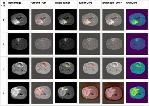
Class activation maps in convolutional layers can be seen and assigned weights using the methods known as 3D class activation mapping (3D-CAM) and 3D gradient-weighted class activation mapping (3D-Grad-CAM). These methods were developed to address complications posed by the presence of correlations and interactions in the data. However, the limited resolution of the convolutional layers slows progress. The amount of detail needed for the exact identification of relevant areas may be lost when using upsampled heatmaps. Because the baseline method must perform a forward pass for each voxel, it can be more computationally efficient. In 3D-CAM, a single forward pass can generate a heatmap but at a high cost in terms of both time and the need for retraining. In Figure 9, the presented image shows the results of Grad-CAM accompanied by a heatmap representation in conjunction with the corresponding ground truth. The heatmap emphasizes specific regions within the input image where the model is pivotal for its prediction. On the contrary, the term “ground truth” pertains to the authentic annotated information or labels linked with the image. This information is integral to comprehending the influential areas within the input image that contribute significantly to the model's decision-making process. Such insights facilitate a more thorough analysis of the behaviour and performance of the model.

Figure 9. Visualization of Input Image, Ground Truth, Whole tumour, Tumor core, Enhanced Tumor, and Grad-CAM highlighted.

7. Conclusion

In this study, we present a new model for 3D MRI image segmentation. Our model combines two modules: the Swin Block3D module, which is based on a Swin Transformer, and the Conv Block3D module, which is based on a CNN. The Swin Block3D sub-module, built on ViT, captures the global dependence information of the image, whereas the Conv Blocks3D sub-module, which uses convolution, captures the local dependence information. By combining these findings, we ensured that all Swin VNETR layers accurately modelled the dependencies of the image. Moreover, Swin VNETR with Non-local block jump connections helps prevent excessive data loss during downsampling in the encoder. In addition, the incorporation of Non-local block significantly contributed to enhancing the overall performance of our model. Through extensive training and evaluation of the BraTS 2021 dataset, we achieved notable improvements in both the Dice coefficient and Hausdorff distance values. Specifically, the Non-local block demonstrated its efficacy by consistently delivering excellent results across various metrics, further underscoring its importance in our model architecture Compared to competing approaches, Grad-CAM's visuals exhibit superior interpretability and model faithfulness. Results from multiple tests demonstrate that our visualizations outperform the state-of-the-art in terms of class discrimination, classifier trustworthiness disclosure, and bias identification in the datasets.

Disclosure statement

No potential conflict of interest was reported by the author(s).