A resampling-based method for effort correction in abundance trend analyses from opportunistic biological records

Abstract

Capsule Resampling data from biological records databases yielded abundance trend estimates better corrected for increasing observation effort.

Aims To correct population trend estimates for the effects of annually changing observation effort in analyses of opportunistic data.

Methods We developed a resampling-based abundance index for analysis of population trends based on opportunistic citizen-science observations. To correct for the huge recent increase in observation effort every year, we resampled (with replacement) a species-specific constant number of records from the data and computed our index. To validate our standardized index, we used counts from the national waterbird census as a benchmark.

Results Over 22 winters (1991–2012), trend estimates based on resampled indices were substantially more similar to waterbird census-based trend estimates than were raw index-based trends. Raw index trends were off by 648% (se 72%) and typically overestimated trends, while trends computed from standardized indices were off by only 125–131% (se 12–13%) and over – and underestimated trends about equally frequently. Hence, our method of effort correction reduced the bias in trend estimates by a factor 5.

Conclusion Our resampling method may be useful for improving trend analyses from collections of opportunistic biological records, as they become increasingly available, especially via the internet.

The Convention on Biological Diversity (1993) 20 years ago emphasized the importance of biodiversity in global policy and a large number of signature states have committed themselves to assessing status and trends of their biodiversity by implementing monitoring programmes (Gregory et al. 2005). However, biodiversity monitoring is a challenge because large-scale, well-designed surveys are very costly. Even with large contributions from volunteers only a handful of the most popular taxa, such as birds, can realistically be monitored in depth and over a long time period. Moreover, large-scale bird surveys typically include only breeding birds, such as the breeding bird surveys in the UK (BBS, bto.org) or in Switzerland (MHB; Schmid et al. 2004). Apart from coordinated counts of waterbirds in winter, which are well established across Europe and beyond (wetland.org; Kuijken 2006, Keller 2011), standardized large-scale monitoring programmes for birds outside the breeding season are rare. This is true even for countries with large numbers of field ornithologists, and much more so in the majority of countries worldwide that do not have a relatively high density of birdwatchers.

In addition to designed monitoring projects, the collection of opportunistic observations in citizen-science projects provides information on biodiversity, and in countries with few observers or for taxa other than birds, this is often the only information available for rarer species. We define opportunistic observations as those which arise by an unspecified, non-systematic observation process, that is not defined by a prescribed and known sampling design. A salient feature of opportunistic surveys is their non-random and generally unknown sampling effort in space and in time. Hence, strictly speaking, the ability to make an inference from the sample of available data to a wider statistical population, such as the bird population in an entire country, is lost.

Recently, internet-based systems for data entry, management and simple analysis have been developed in many countries (e.g. birdtrack.net, worldbirds.org, ebird.org, observations.org and the family of ornitho sites used in several west and central European countries including ornitho.ch in Switzerland). The ease with which information can be entered, summarized and shared with others has been a tremendous encouragement for naturalists to make their observations available and possibly even to increase their observation activities. Hence, the number of people who record their observations and possibly also the intensity with which they watch (e.g. the duration of trips) has greatly increased over the years. A particularly striking example of this is shown in Fig. 1 in Boakes et al. (2010), which compares the number of records and of species recorded for the pheasant family in different data sources, including museum records, the literature, Atlas data and birding trip reports contained on two internet sites that specialize in collecting this latter type of information (travellingbirder.com and birdtours.co.uk). Less than 20 years after their inception, such internet databases with online reporting are now among the major data sources for biodiversity data worldwide. There can be little doubt that this development will continue and in the future, internet-based collections of opportunistic data will likely become the major global source of information on distribution and abundance for most species, avian or otherwise, which are commonly watched by naturalists.

Opportunistic data provide valuable information on the occurrence of species. In the absence of standardized monitoring schemes the ability to use such data to estimate trends would be helpful. The increase in information, however, makes it more and more difficult to tell apart a genuine trend in abundance or distribution from mere changes in the effort with which a species is observed. This is a challenge even with highly standardized surveys (Brown et al. 2007, Hochachka & Fiedler 2008, Kéry et al. 2009); with opportunistic data, the problem is magnified enormously. Clearly, when more people are looking for a species, or when they are looking harder (for instance, longer, or for more days during a particular trip) or at more sites, then higher numbers are likely to be reported or the species is likely to be recorded from more sites than before. This may happen even in the absence of any underlying positive trend in abundance or distribution. Of course, it may even be possible that a genuine population decline is reflected in the observed data by a strong increase, mediated by increased observation effort. Thus, despite the increasing quantity of the data, citizen-science data sets are qualitatively inferior in comparison to data from designed biodiversity sampling schemes. Patterns in citizen-science data are very much the result of confounding temporal patterns in a studied population with the patterns in the number and the activities of the human observers (Tulloch & Szabo 2012). We call the latter two collectively observation effort. Opportunistic observations therefore present great challenges for quantitative analyses, but nevertheless, they clearly have a potential for assessments of long-term trends of biodiversity (Conrad & Hilchey 2011, Snäll et al. 2011, Tulloch et al. 2013). Methods are badly needed that can cope with this challenge, i.e. that can tease apart patterns in distribution or abundance from mere patterns in observation effort.

For species distribution data (i.e. ‘presence/absence'), we have recently developed a capture–recapture-type of effort correction (Kéry, Gardner et al. 2010, Kéry, Royle et al. 2010; see also Altwegg et al. 2008, van Strien et al. 2010). This method recognizes that when there are clearly documented replicate observations (e.g. when the outcome of every survey at a site is recorded as the ‘presence' or the ‘absence' of a species) over a short time interval (for instance, a breeding season), over which the occurrence state of a species can be assumed constant (the ‘closure' assumption), within-season variation of detections ( ‘presences') and non-detections (‘absences') of a species at each site allows an estimate of detection probability. Detectability contains all per-survey effects of varying observation effort and thus represents the direct link between the observed patterns and the underlying true patterns in distribution or abundance. Estimating detection probability using a site-occupancy model (MacKenzie et al. 2002, 2003), we were thus able to fully correct for annual variation in effort, because the second component of effort, the number of surveys, is simply an issue of sample size within this modelling framework.

In addition, other methods to standardize species distribution data have been proposed that are not based on an explicit sampling mechanism, but instead attempt at standardizing the observed number of occurrences or the observed species richness by some explicit measure of effort (Harrison et al. 1997, Szabo et al. 2010, Balmer et al. 2013). They may all be valuable to standardize citizen-science data for changing effort.

However, distribution data are less information-rich about population trends than are abundance data (i.e. counts; Pollock 2006). That is, with few exceptions, trends in abundance will be reflected by trends in the distribution, but the latter are less sensitive to population change than are trends in abundance. Moreover, many populations are very dynamic (e.g. migrating birds at stopover sites), violating the closure assumption. Still, indices can be constructed that contain information about changes in population size, such as raw counts or some standardized counts of the catch-per-unit-effort type (Williams et al. 2002). Unfortunately, patterns in such indices, such as temporal trends, can be similarly confounded by changes in observation effort.

Here, inspired by rarefaction techniques (Simberloff 1972), we develop a simple resampling method as an attempt to correct population indices derived from opportunistic data for the effects of annual variation (typically increases) in observation effort. Our basic premise is that the number of records (or of recorded visits of observers to a site; see below) in a database can be considered to represent a measure of observation effort. Thus, to correct for annual variation in effort, for each year we repeatedly draw a random sample of constant size from all records and compute the index value. By drawing (with replacement) a sample equal to the number of records in the year(s) with least effort, we can compute what the index value would have been with a constant observation effort. Trends can then be estimated for such standardized annual indices, which should be less or possibly even not affected by increases in observer effort over time.

We use opportunistic data collected in Switzerland by the Swiss Ornithological Institute during winter over 22 years (1991–2012) to illustrate and evaluate our resampling method. Population trends outside the breeding season are not documented by standardized schemes for the whole of Switzerland and all species. The only such programme is the national waterbird census (Keller 2011). Trends calculated from the waterbird census are considered to give reliable population trends for waterbirds in winter (Keller 2011). We therefore use these trends to compare the results of the standardized indices from opportunistic data, calculated for the same time period within a year as the waterbird census.

METHODS

Data sources

Our opportunistic biological records were collected as part of the Swiss ornithological ‘Informationsdienst’ (ID, or ‘information service', Zbinden & Schmid 1995, also see Kéry, Royle et al. 2010), a national citizen-science scheme run by the Swiss Ornithological Institute, where enrolled volunteers send us their bird observations. Online reporting was introduced in 2007. Information available for every record include species identity and number of birds observed, date and site (at 1 km² accuracy), and observer identity. Most observers send in individual records and not complete lists, but enrolled observers commit themselves to submit all records of a list comprising about 120 rare and uncommon bird species (called category A species) and rare and uncommon breeding species during the breeding season (category B species). Records of all others, called category C species, are submitted at the observer's discretion. Thus, for A species (and B during the breeding season), the combined records can be considered as equivalent to complete species lists and the number of records can be taken as a measure of observation effort, while for C species, the use of all records as a measure of effort may be more debatable. For the winter period, which is considered in this paper, category B species are equivalent to those of category C, i.e. they are recorded at the observer's discretion. Fifty-six wetland species that are systematically recorded in the waterbird census (Keller 2011) were included in our analysis. Only records where observers noted the number of observed individuals were included in the analysis, but not those indicating only recorded presence of the species, which is often the case for species of category C when complete lists are submitted.

The Swiss waterbird census consists of two country-wide counts, in mid-November and in mid-January, and covers all large and medium-sized lakes and rivers and a large number of smaller waterbodies (Keller 2011). Coverage of sites reached almost 100% every year during the time period considered. Therefore, the national total was used for the trend analyses without correction for missing sites. Foreign parts of cross-border lakes were not included to make the spatial unit as comparable to that of the opportunistic ID data as possible.

The SOPM abundance index

Many previous analyses of the annual change in the occurrence and abundance of passage migrants or wintering birds in Switzerland informed by opportunistic ID data have been based on the SOPM index of abundance (Zbinden & Schmid 1995). SOPM (‘Summe der Ortspentadenmaxima') is an acronym for the German description of its computation: for a target species, it is the sum of the maximum number of birds recorded per site (= 1 km² quadrats) and five-day period (= pentade; Berthold 1973). The SOPM index may be computed for any area (e.g. the whole country, a region or a certain wetland) or time period (e.g. the whole year, a winter or a single month). The construction of the SOPM index is motivated by the wish for a measure of the total number of individuals that use Switzerland especially for migration stopover or wintering. Taking the maximum number recorded within a site is an approximation to the true number of birds present. Considering the maximum only once within five days is meant to confer some protection against multiple counting of the same birds by different observers at the same site during the same day or during consecutive days (by the same or different recorders).

The SOPM index is sensitive to four quantities: (1) the number of sites where and (2) of five-day periods when a species occurs, (3) the abundance patterns of a species over space and time and (4) the observed maximum count. Of course, a species will never be recorded at all combinations of sites and five-day periods where it occurs and typically not all birds present per spatio-temporal unit will be detected (i.e. detection probability will be <1). Hence, (1), (2) and (4) are all affected by what we call observation effort: e.g. number of observers, number of visits, duration of visits, etc. Variation in the number of sites visited by observers, the number of five-day periods with observations and how well the maximum count agrees with the true total number of birds present all represent nuisance variation in the SOPM index that should be minimized as far as possible.

In recent years, we observed that our original SOPM index suggested increases in abundance even for species for which other, independent data strongly suggested declines. It became clear that the increased observation effort, especially after the start of the online reporting platform ornitho.ch, which led to greatly increased numbers of records in the ID database (Fig. 1), was boosting the SOPM index, presumably through its effects in (1), (2) and (4) above. We therefore looked for a method to statistically control for the effects of increasing observation effort and so developed a resampling-based effort standardization for our SOPM index and of the ensuing trend estimates that are based on this index.

Figure 1. Number of records per year in the Swiss ID data base of opportunistic observations contributed by enrolled volunteers during 1991–2012.

Standardizing the index by resampling records or by resampling visits

We devised two variants of a standardized SOPM index by repeatedly resampling a constant amount of data, representing a constant observation effort, in every year and recalculating the index every time. In this rarefaction (Simberloff 1972) or non-parametric bootstrap (Dixon 2002) procedure, the size of the sample from which the SOPM index is calculated is kept constant over the years in an attempt to simulate a situation where observation effort does not change over the years. For every year, we resampled (with replacement) the data and recalculated the SOPM index 100 times and used the mean and standard deviation as the standardized SOPM index and its bootstrap standard error (se). To improve measurement of observation effort, as well as to reduce the computational burden, we applied a spatio-temporal restriction to the data analysed: for each species, we included only sites (1 km² quadrats) where the species had ever been observed, i.e. where at least one record existed for the entire time period considered. In addition, we included only five-day periods in which a species was ever recorded in Switzerland. We expect that these restrictions would ‘sharpen' the index, because effort is measured only for those sites and times where the target species actually occurs.

We envisioned two ways of expressing ‘observation effort' in the standardized SOPM index: variant (1) uses the number of records (species observations) and variant (2) uses the number of recorded visits per 1 km² quadrat, day and observer. In variant 2, all but one record per day, 1 km² quadrat and observer were discarded prior to bootstrapping.

Since we had no a priori, nor any data-based reasons to prefer one standardized index over the other, we also computed a mean standardized index, by averaging over the total of 200 bootstrap samples of the standardized indices of variants 1 and 2 and treating their standard deviation as the se of the average index. This is similar in spirit to model averaging (Burnham & Anderson 2002): the two standardized indices (variant 1 and variant 2) can be seen as two models for effort correction and by averaging we account for model selection uncertainty. By basing the averaging on a sample of bootstrap replicates, computation of the uncertainty (se) of the mean is readily accomplished in the same way as in Markov chain Monte Carlo techniques in Bayesian analyses (Brooks 2003).

Estimation, comparison and summaries of trends

We used data from the 22 winters 1991/1992–2012/2013 for 56 wetland species from the opportunistic ID and the waterbird census to compare trend estimates from linear regressions for raw and standardized SOPM indices in opportunistic ID data with the corresponding trend estimate from the waterbird census. The two national wetland census counts take place on the weekends closest to 15 November and 15 January. To achieve maximum comparability we calculated the SOPM indices based on opportunistic ID data for the time period from 7 November to 20 January. Seven species were included in the waterbird census only from 1996/1997 onwards; hence, we similarly restricted the opportunistic ID data for these species to ensure maximum comparability with the waterbird census benchmark. For waterbird census and raw SOPM indices, a linear regression model was fitted directly. However, a precision-weighted regression was necessary for variants 1 and 2, and their average, of the standardized SOPM index to accommodate the fact that not every annual standardized index value was equally reliable (i.e. had the same bootstrap se). In a precision-weighted analysis, the error contains two components: a residual accounting for a failure of the annual values to lie exactly on a straight line, plus an estimation of the error component which was assumed known and given by the bootstrap se of the annual index.

To compare SOPM-based trends from the opportunistic ID data with those computed from the assumed accurate waterbird census benchmark data, we computed the signed relative difference (with respect to the waterbird census trend estimate, expressed as a percentage) of the trend estimates for the SOPM indices for the opportunistic ID data as follows for species s (s = 1 … 56):where beta_s is the trend estimate obtained from fitting a (possibly weighted) simple linear regression model to the (possibly standardized) SOPM indices for species s and beta.wbc_s is the corresponding trend estimate from the waterbird census for that species.

Precision-weighted linear regression is straightforward in a Bayesian mode of analysis using the BUGS language; for code see McCarthy & Masters (2005). For this reason and for the ease with which ses or Bayesian confidence intervals can be computed for functions of parameters (Kéry 2010), we conducted these analyses in Bayesian modelling software JAGS (Plummer 2003). We chose default vague priors that resulted in estimates largely determined by the data (Kéry 2010, Kéry & Schaub 2012) and ran Markov chains with sufficient burn-in period and overall length that convergence was reached (indicated by values of the Brooks–Gelman–Rubin statistic < 1.1; Brooks 2003). We report posterior means and standard deviations as Bayesian point and se estimates, except for the relative differences of trend estimates which had very skewed posterior distributions, so we characterized them by 25% trimmed means and standard deviations. The significance of a parameter was judged by whether zero was inside or out of a 95% Bayesian percentile-based confidence interval.

To summarize (over all 56 study species) the estimated relative differences of trend estimates, we used a simplified version of the weighted trend model with an intercept only, which we fitted again in programme JAGS. A summary over all species of the relative differences between trend estimates does not keep track of the sign of the trends, and an average relative difference close to zero may simply come about by similar numbers of negative errors (underestimates) and positive errors (overestimates), relative to the waterbird census benchmark. Thus, we also made this comparison for the absolute, relative difference in the trends, i.e. for the distance of the SOPM-based trend estimates from opportunistic ID data, relative to the waterbird census-based trend estimates. Species of categories B and C showed a much larger increase in records in particular after the introduction of the online reporting platform ornitho.ch in 2007 than species of category A. We therefore conducted these latter comparisons separately for category A species and those in categories B and C.

R resampling and BUGS weighted regression code can be obtained on request from the second author.

RESULTS

Based on waterbird census data, 36 among the 56 study species increased over the 22 winters (1991/1992–2012/2013) and 20 decreased, although increases were significant in only 21 and decreases in 8 (online Appendix 1). Based on raw SOPM indices, trends for 46 species had a positive sign (and were significant in 37) and 10 had a negative sign (3 significant). The number of positive trend estimates based on the standardized SOPMs of variants 1 and 2 and their average were 31 (of which 22 significant), 25 (11 significant) and 27 (17 significant), respectively, while for negative values the respective figures were 25 (9), 31 (14) and 29 (10). Thus, raw index-based trend estimation identified many more population increases than did trend estimation based on the standardized indices. In contrast, differences between the two SOPM variants were small.

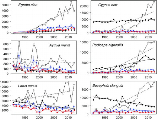
For many category A species with increasing trends according to the waterbird census, the standardized SOPM indices were much closer to those of the waterbird census than the raw SOPM index, which is illustrated by the Great White Egret Egretta alba (Fig. 2, graphs for all species see online Appendix 2). For B and C species that were increasing this was true as well, as illustrated by the Mute Swan Cygnus olor. The raw SOPM indices not only overestimated the magnitude of the increase but seemed to indicate a sudden change in the slope at the time of the introduction of the online reporting platform ornitho.ch, whereas both the waterbird census and the standardized SOPM indices indicated a more continuous trend. For Black-necked Grebe Podiceps nigricollis, on the other hand, the standardized SOPM indices indicated a smaller increase than the waterbird census. For species occurring in small numbers, which often fluctuate between years, illustrated by Greater Scaup Aythya marila, standardizing the SOPM indices tended to reduce the amount of the fluctuation although the peaks remained visible. For abundant but declining categories B and C species, e.g. Common Goldeneye Bucephala clangula the contrast between the trends was most striking, with the strong decline visible from the waterbird census data being opposed to an equally strong increase in the raw SOPM index. For these species, the standardization reduced the slope to a small but not significant increase but was not able to detect a negative trend. For the Mew Gull Larus canus in category A, however, the standardization changed the strong increase in the raw SOPM trend to a significant decline corresponding to the waterbird census trend.

Figure 2. Comparison of annual indices and linear regressions fitted to them for November and January waterbird census counts and raw SOPM indices, as well as the two variants of SOPM indices that were standardized by resampling (variant 1: resample records, variant 2: resample visits) for six example species (left column: A category species, right column: B or C category species; see text). Observed counts or SOPM indices and trend lines are shown for waterbird census data (black filled circles, solid line), raw SOPM index (open circles, dashed line) and standardized SOPM indices (variant 1: blue, variant 2: red). Error bars in standardized SOPM indices represent 1 se. For plots of all species, see the supplementary online materials).

Summarizing the results for all 56 species, Fig. 3 shows the pairwise comparison of the log-transformed, absolute trend estimates based on the four SOPM indices and the waterbird census-based estimates. While the trends based on the raw SOPM indices were always too extreme (high) compared to the waterbird census-based trends (Fig. 3a), those based on the standardized SOPM indices appeared to be fairly unbiased, regardless of whether we considered variant 1, variant 2 or the average of the two standardized indices (Fig. 3b–d).

Figure 3. Scatterplots of the absolute trend estimates (log-transformed) for 56 wintering wetland species in Switzerland based on five data sets/analyses: trends for waterbird census data on the x axis and on the y axis trends based on unstandardized (raw) SOPM indices (3a), standardized indices of variant 1 (resampled records; 3b), standardized indices of variant 2 (resampled visits; 3c) and the average of the two standardized indices (3d). Horizontal grey lines show the values for no trends (i.e. 0) and the diagonal grey line shows equality between two sets of trend estimates.

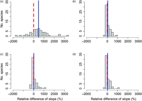
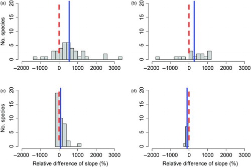
The relative difference (in per cent) between the opportunistic ID data-based SOPM trend estimates and the estimated waterbird census trends for the raw SOPM trends ranged from −1599% to 3194%, with the average estimated in a weighted regression as 449% (se 103%; Fig. 4a). Thus, on average the raw SOPM-based trends were much higher than the trends estimated from waterbird census data. In contrast, the relative differences between waterbird census trends and the trends from the three standardized sets of SOPM indices were much less variable and ranged only from −224% to 907% (average 13%, se 25%) for variant 1 (Fig. 4b), from −406% to 1023% (average −21%, se 24%) for variant 2 (Fig. 4c) and from −204% to 969% (average 0%, se 25%) for the average standardized SOPM index (Fig. 4d). Thus, compared to the waterbird census benchmark, over – and underestimated trends computed from standardized SOPM indices cancelled out almost exactly.

Figure 4. Comparison of relative differences (in per cent of the waterbird census-based trend) of SOPM-based trends computed from opportunistic ID data. (a) Raw SOPM index; (b) standardized SOPM index (variant 1: resampled records); (c) standardized SOPM index (variant 2: resampled visits) and (d) mean of the two standardized SOPM indices. The dashed red line indicates a value of zero, which corresponds to perfect agreement of the trends. The blue line shows the average relative difference.

The absolute relative difference in raw SOPM trends ranged from 3% to 3194% with the average estimated in a weighted regression at 648% (se 72%). In contrast, the relative distance between the waterbird census-based trends and the trends from the three standardized sets of SOPM indices ranged from 1% to 907% (average 125%, se 13%) for variant 1, from 13% to 1023% (average 131%, se 12%) for variant 2 and from −3% to 969% (average 125%, se 13%) for the average standardized SOPM index. Hence, estimating population trends from standardized SOPM indices reduced the bias (the proportional distance to the waterbird census benchmark trend) by a factor 5 compared to the trends computed from the raw SOPM index.

Comparing the effectiveness of our index standardization between species of category A and those in categories B and C (Fig. 5) revealed that standardization was on average similarly effective for both types of species: the reduction in bias in trend estimates (represented by the difference between the blue line and the dashed red line) was similar for both species groups when going from the unstandardized index (Fig. 5a and b) to the standardized indices (Fig. 5c and d). However, the results of standardizing were even more consistently beneficial for species in categories B and C, as shown by the much reduced spread in Fig. 5d.

Figure 5. Comparison of relative differences (in per cent of the waterbird census-based trend) of SOPM-based trends computed from opportunistic ID data separated for the 40 type A and 16 type B or C species; see text for explanation. (a) Raw SOPM index for species A; (b) raw SOPM index for species type B and C; (c) standardized SOPM index for species A and (d) standardized SOPM index for species type B and C. The dashed red line indicates a value of zero, which corresponds to perfect agreement of the trends. The blue line shows the average relative difference.

DISCUSSION

We proposed a rarefaction or resampling method to standardize abundance trend estimates based on opportunistic data by correcting for variable observation effort. We validated our method by comparing effort-standardized trends from our opportunistic ID data with trends estimated from the national waterbird census (Keller 2011). For many wintering wetland species, the Swiss waterbird census in mid-November and mid-January is based on an almost exhaustive spatial sample and is therefore likely to produce reliable assessments of the trends of wintering populations. We tried to maximize temporal and spatial congruence between the opportunistic and the waterbird census data by restricting the former in space and in time for each species. Perfect congruence may be impossible to achieve, but we were unable to find any two independent avian data sets in Switzerland that were only nearly as congruent as these two. We believe that they are sufficiently congruent to warrant use of the waterbird census as a benchmark for the opportunistic data.

The comparison of the effort-corrected abundance trends with trends derived from the standardized waterbird census revealed a five-fold improvement (in terms of bias) in trend estimates based on standardized abundance indices over trends estimated from a raw abundance index. Typically, standardizing the index reduced the slope of the trend, often resulting in a change from a significant positive trend to a non-significant one corresponding to the result from the waterbird census. In the example of the Mew Gull, this even correctly led to a significant negative trend as in the waterbird census. Complete consistency between the trend classifications for all three indices was found for 14 species, two of which, Red-necked Grebe Podiceps grisegena and Common Eider Somateria mollissima showed a significant negative trend, the others no trend. All these species are rare category A species usually observed in groups of fewer than ten individuals. But even for these rare species the trend estimates, even though not significant, were more consistent with the waterbird census trends than the raw indices.

We found differences between complete species list data (represented in our scheme and for the purpose of the analysis presented here by species of category A) and all other data (represented in winter by B and C species). For B and C species, the number of records in winter increased particularly strongly after the establishment of our online reporting platform ornitho.ch in 2007. Effort-corrected trends for B and C species were of similar or even better quality as those for A species. However, out of the six species with contradicting trend classification, five belonged to the B or C category: for Tufted Duck Aythya fuligula and Common Pochard Aythya ferina the negative trend found in the waterbird census remained significantly positive even for the mean standardized SOPM index, for Common Goldeneye the classification was changed from significantly positive in the raw index to no trend in the mean standardized one, failing to pick up the decline as well. The trend was reversed only for the Mew Gull, as discussed above. For Mallard Anas platyrhynchos and Eurasian Teal Anas crecca the standardization seemed to ‘overcompensate' the index, resulting in a significant negative trend in the mean standardized index as opposed to the significant positive trend in the waterbird census. Unlike the Mew Gull, the five duck species belong to the most abundant wintering waterbirds in Switzerland with populations of 6000 (Common Goldeneye) to over 100 000 (Tufted Duck) individuals during the study period. In online portals, they are more likely to be recorded with an absolute number of birds seen where they occur in small groups only, whereas large concentrations are not counted. This clearly indicates that for abundant and widespread species calculating trends from opportunistic data is problematic. Differences in reporting rates of rare and common species were also suspected as a cause for a mismatch between results from the (designed) Swedish Bird Survey and the opportunistic data from the ‘Species Gateway' (Snäll et al. 2011).

We presented two methods of effort correction by resampling either records (variant 1) or visits (variant 2). Variant 1 should be sensitive to changes in the number and in the ‘quality' of visits. For instance, if visit duration increases over the years, we would expect an increased number of overall records, including the target species, and this would be corrected for by directly resampling records (species observations). On the other hand, in variant 1, there is a confounding of the standardized index with the species richness of a site, since a visit at a species-rich site may easily contribute 40 records per day, year and observer, while a visit at, say, a high-altitude site might hardly contribute more than a single record. Thus, if the total number of individuals of all recordable species changes over time, or if over time, sites with different total numbers of individuals of these species tend to be visited, we might erroneously measure a change in effort and our standardized index would be biased. In contrast, variant 2 of the standardized SOPM index counts a visit by the same observer in a 1 km² quadrat per day only once. Thus, it would be expected to be insensitive to any changes in the overall abundance of the species present, because it makes the assumption that the ‘quality' (such as duration, number of observers and quality of observers) of visits or sites does not change over the years. In contrast, if observers tend to stay longer at a site over the years, representing an increase in effort, this will violate the assumption of variant 2 that the visit ‘quality' stays constant over time. In our study we found very similar inferences about trends when using the two variants of effort standardization, suggesting that neither the ‘quality' of visits nor the total population sizes of the study species have changed over the study period. In other applications, this may differ however, and how effort is best measured must probably be decided on a case by case basis.

Trends are rates of change over time and may be expressed in many different ways; objectives of trend estimation may also vary (Thomas 1996). We used the simplest possible trend model (a linear regression), because this met our objectives. However, a resampling effort correction will also be useful to other models of trend, such as generalized additive models (Fewster et al. 2000, Dennis et al. 2013) or state-space models (Knape et al. 2009, Kery & Schaub 2012, chap. 5), because their trend estimates will be biased as well when observation effort changes over time.

Our new method of correcting abundance indices for observation effort enables us to gauge population trends of many avian species that are not well enough surveyed by other, established monitoring schemes, such as the breeding bird survey MHB (Schmid et al. 2004). Importantly, it also enables us to assess trends for species that are not at all covered by our designed monitoring schemes, especially species that use Switzerland for stopover or for wintering.

Possible improvements and developments of our method include the ‘sharpening' of the index by restricting resampling with respect to space, time, taxonomy or habitat and its application in other settings, e.g. to seasonal patterns. For example, we might measure observation effort for each species separately, e.g. for an owl species, we might restrict the number of visits to those when other nocturnal species were observed or for a wetland species, we could only use records of other wetland species. The spatio-temporal scale of the analysis is also likely to be relevant. Our spatio-temporal unit was 1 day and 1 km², but perhaps another grain size of aggregation, e.g. 2 days and 0.25 km², might give better results for some species. On the other hand, such a high resolution might be problematic for highly mobile passage migrants. This can be experimented with to optimize the analysis protocol.

The idea of resampling constant amounts of data for effort correction can be applied more widely, e.g. to compare phenology profiles between different time periods (Gerber et al. 2011) correcting for possibly different seasonal distribution of observation effort between periods. Resampling phenological observations could improve estimation of the seasonal use of stopover sites and might be important in climate change studies, to correct for variable effort phenological indices based on bird occurrence.

Correcting for variable observation effort in space and time is fundamental for making the best inferences about spatio-temporal patterns in abundance. It is especially important when dealing with opportunistic citizen-science data, because without a prescribed and known sampling design, effort is likely to be especially variable in space and time. In principle, we may distinguish between three types of effort correction: (1) simple resampling-based methods without any direct information about effort (e.g. this study) , (2) covariate modelling of the effects of measured effort covariates (which may include observer identity, e.g. Link & Sauer 2002, 2007, Szabo et al. 2010, Balmer et al. 2013) and (3), an explicit mechanistic description of the observation processes (which may include covariate effects as well; e.g. capture–recapture-types of models; Royle & Kéry 2007, Kéry et al. 2009, Kéry, Royle et al. 2010). Arguably, types 2 and 3 of effort corrections may be superior to simple rarefaction-type of methods, because they exploit additional information available about the observation process. However, a formal comparison would be welcome. We believe that the development of reliable methods for correcting citizen-science data for variable observation effort will be the main methodological challenge for this increasingly super-abundant source of information for many years to come.

SUPPLEMENTAL MATERIAL

Supplementary online Appendices 1 (trend estimates and standard errors for all species) and 2 (plots of annual indices and estimated linear regression lines for all 56 analysed wetland bird species) can be accessed at 10.1080/00063657.2014.969679.

ACKNOWLEDGEMENTS

We thank the thousands of volunteers who have contributed their observations for many decades now. We also thank Will Cresswell and two anonymous referees whose comments have much improved the original draft of our paper.

REFERENCES

- Altwegg, R., Wheeler, M. & Erni, B. 2008. Climate and the range dynamics of species with imperfect detection. Biol. Lett. 4: 581–584. doi: 10.1098/rsbl.2008.0051
- Balmer, D.E., Gillings, S., Caffrey, B.J., Swann, R.L., Downie, I.S. & Fuller, R.J. 2013. Bird Atlas 2007–11: The Breeding and Wintering Birds of Britain and Ireland. BTO Books, Thetford.
- Berthold, P. 1973. Proposals for the standardization of the presentation of data of annual events, especially of migration data. Auspicium 5: 49–57.
- Boakes, E.H., McGowan, P.J.K., Fuller, R.A., Chang-Qing, D., Clark, N.E., O'Connor, K. & Mace, G.M. 2010. Distorted views of biodiversity: Spatial and temporal bias in species occurrence data. PLoS Biology 8: e1000385. doi: 10.1371/journal.pbio.1000385
- Brooks, S.P. 2003. Bayesian computation: a statistical revolution. Phil. Trans. Royal Soc. London, Series A 361: 2681–2697. doi: 10.1098/rsta.2003.1263
- Brown, W.S., Hines, J.E. & Kéry, M. 2007. Survival of timber rattlesnakes (Crotalus horridus) estimated by capture-recapture models in relation to age, sex, color morph, time, and birthplace. Copeia 2007: 656–671. doi: 10.1643/0045-8511(2007)2007[656:SOTRCH]2.0.CO;2
- Burnham, K.P. & Anderson, D.R. 2002. Model Selection and Multimodel Inference: Practical Information-theoretic Approach. Springer, New York.
- Conrad, C.C. & Hilchey, K.G. 2011. A review of citizen science and community-based environmental monitoring: issues and opportunities. Environ. Monit. Assess. 176: 273–291. doi: 10.1007/s10661-010-1582-5
- Dennis, E.B., Freeman, S.N., Brereton, T. & Roy, D.B. 2013. Indexing butterfly abundance whilst accounting for missing counts and variability in seasonal pattern. Meth. Ecol. Evol. 4: 637–645. doi: 10.1111/2041-210X.12053
- Dixon, P.M. 2002. Bootstrap resampling. In El-Shaarawi, A.H. & Piegorsch, W.W. (eds) Encyclopedia of Environmetrics, Vol. 1: 212–220. Wiley, New York.
- Fewster, R.M., Buckland, S.T., Siriwardena, G.M., Baillie, S.R. & Wilson, J.D. 2000. Analysis of population trends for farmland birds using generalized additive models. Ecology 81: 1970–1984. doi: 10.1890/0012-9658(2000)081[1970:AOPTFF]2.0.CO;2
- Gerber, A., Leuthold, W. & Kéry, M. 2011. Der Bienenfresser Merops apiaster in der Schweiz: Durchzug und Bruten. [The European Bee-eater Merops apiaster as a passage migrant and breeding species in Switzerland.] Ornithol. Beob. 108: 101–116.
- Gregory, R.D., van Strien, A., Vorisek, P., Gmelig Meyling, A.W., Noble, D.G., Foppen, R.P.B. & Gibbons, D.W. 2005. Developing indicators for European birds. Phil. Trans. Royal Soc. London, Series B 360: 269–288. doi: 10.1098/rstb.2004.1602
- Harrison, J.A., Allan, D.G., Underhill, L.G., Herremans, M., Tree, A.J., Parker, V. & Brown, C.J. (eds) 1997. The Atlas of Southern African Birds. BirdLife South Africa, Johannesburg.
- Hochachka, W.M. & Fiedler, W. 2008. Trends in trappability and stop-over duration can confound interpretations of population trajectories from long-term migration ringing sites. J. Ornithol 149: 375–391. doi: 10.1007/s10336-008-0282-1
- Keller, V. 2011. La Suisse, refuge hivernal pour les oiseaux d'eau. Avifauna Report Sempach 6, Station ornithologique suisse, Sempach.
- Kéry, M. 2010. Introduction to WinBUGS for Ecologists. – A Bayesian Approach to Regression, ANOVA, Mixed Models and Related Analyses. Academic Press, Burlington, MA.
- Kéry, M., Dorazio, R.M., Soldaat, L., van Strien, A., Zuiderwijk, A. & Royle, J.A. 2009. Trend estimation in populations with imperfect detection. J. Appl. Ecol. 46: 1163–1172.
- Kéry, M. & Schaub, M. 2012. Bayesian Population Analysis Using WinBugs. A Hierarchical Perspective. Academic Press, Elsevier, Waltam, MA.
- Kéry, M., Gardner, B. & Monnerat, C. 2010. Predicting species distributions from checklist data using site-occupancy models. J. Biogeogr. 37: 1851–1862.
- Kéry, M., Royle, J.A., Schmid, H., Schaub, M., Volet, B., Häfliger, G. & Zbinden, N. 2010. Site-occupancy distribution modeling to correct population-trend estimates derived from opportunistic observations. Conserv. Biol. 24: 1388–1397. doi: 10.1111/j.1523-1739.2010.01479.x
- Knape, J., Jonzen, N., Skold, M. & Sokolov, L. 2009. Multivariate state-space modelling of bird migration count data. In Thomson, D.L., Cooch, E.G. & Conroy, M.J. (eds) Modeling Demographic Processes in Marked Populations. Book Series: Environmental and Ecological Statistics Series, Vol. 3: 59–79. Springer, New York.
- Kuijken, E. 2006. A short history of waterbird conservation. In Boere, G.C., Galbraith, C.A. & Stroud D.A. (eds) Waterbirds Around the World, 52–59. The Stationery Office, Edinburgh.
- Link, W.A. & Sauer, J.R. 2002. A hierarchical analysis of population change with application to Cerulean Warblers. Ecology 83: 2832–2840. doi: 10.1890/0012-9658(2002)083[2832:AHAOPC]2.0.CO;2
- Link, W.A. & Sauer, J.R. 2007. Seasonal components of avian population change: joint analysis of two large-scale monitoring programs. Ecology 88: 49–55. doi: 10.1890/0012-9658(2007)88[49:SCOAPC]2.0.CO;2
- MacKenzie, D.I., Nichols, J.D., Lachman, G.B., Droege, S., Royle, J.A. & Langtimm, C.A. 2002. Estimating site occupancy rates when detection probability rates are less than one. Ecology 83: 2248–2255. doi: 10.1890/0012-9658(2002)083[2248:ESORWD]2.0.CO;2
- MacKenzie, D.I., Nichols, J.D., Hines, J.E., Knutson, M.G. & Franklin, A.B. 2003. Estimating site occupancy, colonization and local extinction when a species is detected imperfectly. Ecology 84: 2200–2207. doi: 10.1890/02-3090
- McCarthy, M.A. & Masters, P. 2005. Profiting from prior information in Bayesian analyses of ecological data. J. Appl. Ecol. 42: 1012–1019. doi: 10.1111/j.1365-2664.2005.01101.x
- Plummer, M. 2003. JAGS: a program for analysis of Bayesian graphical models using Gibbs sampling. Proceedings of the 3rd International Workshop on Distributed Statistical Computing (DSC 2003), March 20–22, Vienna, Austria. ISSN 1609–395X.
- Pollock, J.F. 2006. Detecting population declines over large areas with presence-absence, time-to-encounter, and count survey methods. Conserv. Biol. 20: 882–892. doi: 10.1111/j.1523-1739.2006.00342.x
- Royle, J.A. & Kéry, M. 2007. A Bayesian state-space formulation of dynamic occupancy models. Ecology 88: 1813–1823. doi: 10.1890/06-0669.1
- Schmid, H., Zbinden, N. & Keller, V. 2004. Überwachung der Bestandsentwicklung häufiger Brutvögel in der Schweiz. Schweizerische Vogelwarte, Sempach.
- Simberloff, D. 1972. Properties of the rarefaction diversity measurement. Am. Nat. 106: 414–418. doi: 10.1086/282781
- Snäll, T., Kindvall, O., Nilsson, J. & Pärt, T. 2011. Evaluating citizen-based presence data for bird monitoring. Biol. Conserv. 144: 804–810. doi: 10.1016/j.biocon.2010.11.010
- van Strien, A.J., Termaat, T., Groenendijk, D., Mensing, V. & Kéry, M. 2010. Site-occupancy models may offer new opportunities for dragonfly monitoring based on daily species lists. Basic Appl. Ecol. 11: 495–503. doi: 10.1016/j.baae.2010.05.003
- Szabo, J.K., Vesk, P.A., Baxter, P.W.J. & Possingham, H.P. 2010. Regional avian species declines estimated from volunteer-collected long-term data using List Length Analysis. Ecol. Appl. 20: 2157–2169. doi: 10.1890/09-0877.1
- Thomas, L. 1996. Monitoring long-term population change: why are there so many analysis methods? Ecology 77: 49–58. doi: 10.2307/2265653
- Tulloch, A. & Szabo, J.K. 2012. A behavioural ecology approach to understand volunteer surveying for citizen science datasets. Emu 112: 313–325. doi: 10.1071/MU12009
- Tulloch, A.I.T., Possingham, H.P., Joseph, L.N., Szabo, J. & Martin, T.G. 2013. Realising the full potential of citizen science monitoring programs. Biol. Conserv. 165: 128–138. doi: 10.1016/j.biocon.2013.05.025
- Williams, B.K., Nichols, J.D. & Conroy, M.J. 2002. Analysis and Management of Animal Populations. Academic Press, San Diego, CA.
- Zbinden, N. & Schmid, H. 1995. Das Programm der Schweizerischen Vogelwarte zur Überwachung der Avifauna gestern und heute. Ornithol. Beob. 92: 39–58.