Measuring Dynamic Effects of Remittances on Poverty and Inequality with Evidence from Kosovo

ABSTRACT

This paper investigates dynamic effects of remittances on households’ poverty and income distribution. Using state-of-the-art matching techniques, we measure impacts based on counterfactual scenarios, and make a step forward by applying for the first time a dose-response function approach to assess poverty effects due to variations in the time-length of receiving remittances. Our results suggest that remittances alleviate both absolute and relative poverty levels and lead to a marginal increase in inequality in the case of Kosovo. We further demonstrate that – although poverty reduction effects are stronger in the short-run – remittances have a positive poverty reduction effect over time. These findings have important welfare policy implications for low- and middle income economies with a high dependency on remittances.

KEYWORDS:

• Poverty
• inequality
• migration
• remittances
• dose-response function
• Kosovo

JEL CLASSIFICATION:

• D10
• D31
• I32
• I61

Introduction

Just recently, remittances to low – and middle-income countries rebounded to a record level in 2017 (World Bank 2018). Undoubtedly, migration and remittances have significant implications for growth and poverty alleviation in countries of origin. Despite a considerable number of essential contributions discussing the linkages between remittances and poverty and inequality (Barham and Boucher 1998; Feldman and Leones 1998; Kimhi 2010; Oberai and Singh 1983; Shen, Docquier, and Rapoport 2010; Stark, Taylor, and Yitzhaki 1986; Taylor 1992; Taylor et al. 2005; Taylor, Rozelle, and de Brauw 2003), empirical results are ambiguous and methodological issues persist. Hence, the UN 2030 Agenda for Sustainable Development rightly calls for more scientific-based evidence on migration effects (UN 2015).

In response to this call, our study suggests an innovative combination of econometric methods in order to provide new empirical evidence to the debate on the causal linkages between remittances, poverty and inequality. Specifically, propensity score matching (PSM) techniques and a “dose-response” function approach are combined for the analysis of cross-sectional data. Using counterfactual incomes, the marginal effect of remittances on poverty alleviation and inter-household income distribution are explored. An important contribution of this paper is the extension of poverty analysis to capture the effects of the time length of receiving remittances on the conditional probability of falling below a certain poverty threshold. For this we utilize a state-of-the-art “dose-response” function, with generalized propensity scores (GPS) following the methodology developed by Imbens (2000) and Hirano and Imbens (2004). The application of the method to the case of dynamic effects of remittances on poverty allows for completely new and highly useful insights into longitudinal effects of receiving remittances even in typical cross-sectional research designs. The combination of both methods is applied for the first time to remittances’ analysis in this paper.

The innovative approach is illustrated using data from Kosovo. The country is known for its longstanding outmigration history and migrant-sending communities struck by poverty, extreme unemployment rates and limited livelihood opportunities. Kosovo not only has the lowest GDP per capita in Europe, around USD 3,957 (World Bank 2017), but its economy is highly dependent on remittances. The country ranks fourth among the top ten remittance-dependent European and Central Asian transition economies (World Bank 2018). Despite sizable remittance inflows in the recent years and a large number of beneficiaries, over 25% of Kosovars are considered poor or vulnerable to poverty (IMF 2018). While poverty is characterized by annual cyclicality, inequality is considered to be stable and low in Kosovo compared to other transition countries. In 2015, the Gini coefficient was 0.23 (IMF 2018).

Our paper contributes to the migration literature in two main aspects. Firstly, this study represents the first application of a dose-response estimation with GPS in migration research. Given the scarcity of panel data in migration research, this article opens a new methodological venue for the estimation of migration and remittances effects in absence of longitudinal data.

Secondly, our empirical findings add to previous findings on migration and welfare links undertaken in the context of other regions with similar results (Acosta et al. 2008; Adams 1989; Adams and Page 2005; Möllers and Meyer 2014; Taylor et al. 2005). We utilize a rich household-level data set from the 2011 UNDP Kosovo Remittance Household Survey and provide empirical results that contribute to closing a gap in research by highlighting remittances effects in the highly remittance-dependent, but under-researched Eastern European transition economies.

The paper is organized as follows: after a brief review of the literature on the link between remittances and income inequality as well as poverty in Section 2, we introduce our data and key elements of our innovative methodology in Section 3. Section 4 provides a detailed comparison of migrant and non-migrant households based on our empirical dataset. The key analytical results are presented in Section 5. Section 6 assesses the main findings and concludes with an evaluation on the welfare effects of participation in international labor migration.

Literature Review

The literature on the interrelation of migration and remittances and income inequality provides mixed results. In an early study on the impact of migration on rural development in India, Oberai and Singh (1983) find that remittances have an equalizing effect as they reduce the income gap between the top and bottom income groups not only for migrant sending, but for all rural households. However, most of the evidence points to the contrary effect. Adams (1989) estimates that remittance income has a negative impact on rural income distribution in Egypt in gross and per capita terms. Remittance income benefits the upper-income rural households, which are best positioned to access foreign labor markets. Feldman and Leones (1998) evaluate the specific effects of farm and non-farm income (including remittances) on income inequality and employment opportunities in resource-poor rural areas. Their findings suggest that the effects on income inequality depend on the type of non-farm income and availability of non-farm employment. Remittances as a specific form of non-farm income, the authors argue, increase income inequality significantly.

A study on Mexico by Taylor et al. (2005) shows that international remittances contribute to a slight increase in income inequality, whereas the effects of internal remittances are the opposite. However, in regions with highest shares of migrants, international remittances have an income equalizing effect. Kimhi (2010) estimates the income distribution impact of internal and international remittances in the Dominican Republic, where internal remittances have a stronger adverse marginal effect on rural landless households, while international remittances have a more prominent un-equalizing impact on urban families.

Finally, there is evidence that remittances’ effects on poverty and inequality differ depending on their sources and operationalization of household’s welfare. Shen, Docquier, and Rapoport (2010) maintain that while migration decreases wealth inequality, it increases income inequality. The short-run and long-run effects on income distribution may be of opposite signs depending on the initial distribution of wealth. Conflicting results in income inequality estimates of migration and remittances might furthermore be explained up to a certain extent by ambiguities in the research questions and statistical methods used (Barham and Boucher 1998): if remittances are treated as an exogenous transfer, the influence of remittances on income in recipient communities should be assessed; if, however, remittances are viewed as substitutes for home earnings, then the question is how the observed income distribution compares to a counterfactual scenario without migration and remittances.

When the effect of remittances on household poverty is analyzed, most studies underline that migration and remittances have the potential to increase household income and reduce poverty (Acosta et al. 2008; Adams 2006; Adams and Page 2005; Amare and Hohfeld 2016; Möllers and Meyer 2014; Taylor et al. 2005; Yang and Martinez 2006). In their comparative analysis of household surveys from 71 developing countries, Adams and Page (2005) find an overall positive, poverty decreasing effect of remittances in the context of emerging, remittance-recipient economies. For the case of Ghana, Adams (2006) finds that both domestic and international remittances reduce the level, depth and severity of poverty, whereby the impacts across the three poverty measures differ considerably. In rural Mexico remittances have a poverty reducing effect in regions where the share of migrant households is highest (Taylor et al. 2005). At the beginning of migration, when only a few migrant families have access to foreign labor markets, remittances flow back to the middle and upper-middle income households, which can afford to send their family members abroad. Yet, poor households gain access to migration over time and may benefit from migration as well. In their study on poverty transition in rural Vietnam, Amare and Hohfeld (2016) find that remittances have a positive effect on asset growth but the effects are heterogeneous, depending on the initial welfare and ethnicity of recipient households. Yang and Martinez (2006) find that receipt of international remittances helps to reduce the conditional probability of a household to fall in poverty in the Philippines. So far only very few studies look at the European and Central Asian transition economies, which differ from the traditional development context analyzed by the studies mentioned so far (Gang et al. 2018; Möllers and Meyer 2014).

Some of the mixed results reported above might be the result of methodological issues. Migration studies have to account among others for endogeneity, selection bias, reverse causality and omitted variables bias (McKenzie and Sasin 2007).¹ For this reason, the study of Yang and Martinez (2006) which closely resembles a natural experiment – using the exchange rate shocks before and after the 1997 Asian financial crises – is considered one of the most resounding investigations on the linkages between migrant remittances and household poverty (Adams 2011). Most migration studies, however, rely on ordinary least squares (OLS) regression analysis, even though there are some arguments against doing so. These include, but are not limited to the nature of the data (most migration data are cross-sectional), the existence of hidden and overt bias, and the serious constraints to find appropriate instruments. Few migration studies have ventured into the application of matching techniques to derive treatment effects (examples are: de Brauw, Mueller, and Woldehanna 2018; Ham, Li, and Reagan 2011; Jimenez-Soto and Brown 2012; Möllers and Meyer 2014). Such techniques were successfully validated against other estimation methods (see Citina and Love 2017) and should be better suited to analyze impacts of remittances when they are seen as a substitute for home earnings. Finally, given the mostly cross-sectional data, insights on the longer term and dynamic aspect are widely neglected so far.

Methodology

In the following we explain our method choice. We rely on propensity score matching (PSM) to derive a counterfactual situation for a typical cross-sectional dataset. We further introduce the application of a dose-response function with generalized propensity scores (GPS) as a particularly useful extension of propensity matching. The treatment effects are hence further analyzed by introducing a continuous treatment variable that allows us to capture dynamic effects.

The PSM method is based on the counterfactual framework of causality. It maintains that participants in treatment (migrant households) and control groups (non-migrant households) have potential outcomes in both conditions, one of which is observed and the other which is not observed. Our outcome of interest is the per capita income. The counterfactual framework for a participant i with potential outcomes in both treatment and control condition (denoted as $Y_{0i}$ and$Y_{1i}$) is expressed as:

(1) $Y_i=D_i{Y}_{1i}+(1-D_i)Y_{0i}$(1)

$D$ is a dichotomous variable which indicates the probability of participation in treatment, that is participation in migration, and (1-$D_i$) denotes the probability of not participating in the treatment.

Estimation of propensity scores relies on binary logit or probit models, whereby the choice of the variables that enter the model is validated by existing theories and all those observed variables influencing participation must be accounted for. While there are no standard technical guidelines on how to specify a good model, there are strategies that may improve the predictive power of the model (see e.g. Heinrich, Maffioli, and Vázquez 2010). Following these strategies, our model estimates the selection into migration as a function of the following covariates: age, gender and education of household head, social status (whether head is still working or a pensioner), ethnicity, share of female household members and locational variables such as average shares of remittances at the municipality level and three dummy variables for regions.

For the choice of the matching algorithm, we follow Austin (2014) who advises to use matching without replacement and within a specified caliper, in our case calculated at 0.25*standard deviation of the propensity scores. Based on the regression results (Appendix, Tables A1 and A2), we predict the propensity scores, which measure the probability of participation in migration. The overlap condition is confirmed by a visual inspection of a histogram of the propensity scores for the two groups (Appendix, Figures A1 and A2) and the quality of matching is satisfactory as shown by the visual inspection of the standardized percentages bias before and after the matching (Appendix, Figure A3 and A4). In addition, we estimate covariate percentage bias reduction via STATA’s pstest command (Appendix, Tables A3 and A4).

For our final model, we confirmed that the estimated impacts are robust and unbiased according to Rosenbaum’s sensitivity analysis (Appendix, Table A5).² Propensity score matching analysis is performed in STATA using psmatch2.

We complement the counterfactual framework with a dose-response estimation with GPS as an extension of the previously discussed Rosenbaum and Rubin (1983) matching. Dose-response estimation with GPS allows adjustment for covariate imbalances when the treatment variable is continuous (Hirano and Imbens 2004; Imbens 2000). This new estimation technique captures dynamic effects of remittances on household poverty. In contrast to OLS regression analysis, which assumes constant effects, the estimation of a dose-response function allows us to predict recipient households’ propensity to fall below a poverty line over the time-length of receiving remittances. Applying this extension for the first time in migration research we estimate the probability that a remittance-recipient household falls below the poverty threshold – associated with each value of the continuous dose, i.e. the length of time (years) that the household receives remittances. In doing so, the dose response estimation is a first and important step into the analysis of dynamic migration and remittances effects in absence of longitudinal data.

Imbens (2000) defines propensity scores with multi-valued treatments that is the generalized propensity score, as the conditional probability of receiving a particular level of treatment, for a set of pre-treatment variables.³ Given a random sample of units of size N and an existent vector of covariates X, it postulates that for each level of treatment received T (where T takes on integer values between 0 and K), there exists a set of potential outcomes Y(t). As such, if r(t,x) is defined as the conditional density of treatment given the covariates:

(1) $r\left(t\mathit{,}x\right)=f_{T|X}\left(t|x\right)$(1)

it follows that GPS is estimated as:

(2) $R=r\left(T\mathit{,}X\right)$(2)

The estimation of the GPS is typically done in three steps (Bia and Mattei 2008; Hirano and Imbens 2004; Kluve et al. 2012).

In the first step, the GPS is generated. To generate such score, for a given set of fixed covariates, the conditional distribution of the length of the treatment variable is estimated such as:

(3) $T_i|X_i\sim \mathrm{N}({\beta }_0+{{\beta }_1}^{\prime }{X}_i,{\sigma }^2)$(3)

The GPS are calculated as:

(4) ${\hat{R}}_i=\frac{1}{\sqrt{2\pi {\hat{\sigma }}^2}}\mathrm{e}\mathrm{x}\mathrm{p}\left(-\frac{1}{2{\hat{\sigma }}^2}(T_i-{\hat{\beta }}_0-{\hat{\beta }}_1{X}_i{)}^2\right)$(4)

Our treatment variable, the length of time a household receives remittances, varies from a minimum of 1 year to 43 years.⁴ Following closely Hirano and Imbens (2004), we use the distribution of the treatment variable to create K treatment intervals (Appendix Table A6).⁵

Next, we run the maximum likelihood regression with the treatment variable as our dependent variable (entered in a logarithmic form) and a number of selected covariates (Eq. 3(2) $R=r\left(T\mathit{,}X\right)$(2) ).⁶ We model the conditional distribution of the treatment variable as a function of the following covariates: ethnicity, age and gender of the household head, his education and marital status, employment status, family size, dependency ratio and five regional dummies for the main six administrative regions in Kosovo. The estimated coefficients (${\hat{\beta }}_0$, ${\hat{\beta }}_1$) are presented in Table A7 in the Appendix. These coefficients are used to evaluate the GPS for all sample observations (Equation 4(4) ${\hat{R}}_i=\frac{1}{\sqrt{2\pi {\hat{\sigma }}^2}}\mathrm{e}\mathrm{x}\mathrm{p}\left(-\frac{1}{2{\hat{\sigma }}^2}(T_i-{\hat{\beta }}_0-{\hat{\beta }}_1{X}_i{)}^2\right)$(4) ). In line with Hirano and Imbens (2004), we test that covariate balancing with GPS is successfully attained (Appendix, Table A8).

In the second step, we estimate the conditional expectation of the outcome variable, the conditional probability of falling below the poverty threshold. Such an expectation is expressed as a linear function of two variables, the treatment T and the GPS:

(5) $\beta \left(t\mathit{,}r\right)=E\left(Y|T\mathit{=}t\mathit{,}R\mathit{=}r\right)$(5)

For each household, the observed $T_i$ and estimated $\widehat{R_i}$ is used. In order to allow for a flexible functional form, we use the following approximation:

(6) $\mathrm{E}[Y_i|T_i,R_i]={\alpha }_0+{\alpha }_1{T}_i+{\alpha }_2{T_i}^2+{\alpha }_3{R}_i+{\alpha }_4{R_i}^2+{\alpha }_5{T}_i{R}_i$(6)

The practical implementation of this second step is the following: we regress the outcome variable, the expected conditional probability of being poor, on the generalized propensity scores, the observed value of $T_i$, their squared terms and an interaction term of these two independent variables (Appendix Table A9). In order to validate our poverty estimations, the second step is repeated for a second outcome variable, the expected annual income (per capita equivalized) (Appendix Table A10).

Following Hirano and Imbens (2004), we do not interpret the estimated coefficients of this regression, except for the fact that a coefficient for the generalized propensity scores of a value equal to zero, would be an indication of potential bias in the covariates.

The third and last step in the analysis is the estimation of the dose-response function expressed as:

(7) $\mu \left(t\right)=E[\beta \left\{t\mathit{,}r\left(t\mathit{,}X\right)\right\}]$(7)

The average dose-response function is generated via the estimation of average potential outcomes for each level of treatment t. The average potential outcome at treatment level t is estimated as:

(8) $\mathrm{E}[Y\left(t\right)]=\frac{1}{N}{\sum }_{i=1}^N{\hat{\alpha }}_0+{\hat{\alpha }}_{1}t+{\hat{\alpha }}_2{t}^2+{\hat{\alpha }}_3\hat{r}\left(\mathrm{t},X_i\right)+{\hat{\alpha }}_4{\hat{r}}^2\left(\mathrm{t},X_i\right)+{\hat{\alpha }}_{5}t\hat{r}\left(\mathrm{t},X_i\right)$(8)

The averaging of the conditional expectation over the marginal distribution of r(t,X) (Equation 8(8) $\mathrm{E}[Y\left(t\right)]=\frac{1}{N}{\sum }_{i=1}^N{\hat{\alpha }}_0+{\hat{\alpha }}_{1}t+{\hat{\alpha }}_2{t}^2+{\hat{\alpha }}_3\hat{r}\left(\mathrm{t},X_i\right)+{\hat{\alpha }}_4{\hat{r}}^2\left(\mathrm{t},X_i\right)+{\hat{\alpha }}_{5}t\hat{r}\left(\mathrm{t},X_i\right)$(8) ), corresponds to the dose-response function for treatment level t, which gives the causal interpretation.

We computed the estimation of “dose-response effects” in Stata using the doseresponse module developed by Bia and Mattei (2008). The software program allows the implementation of the technical procedure for the covariate balance check proposed by Hirano and Imbens (2004).

Data and Description of Sample

Our study provides new empirical evidence on the causal linkages between remittances, poverty and inequality by applying the described combination of PSM and dose-response estimations on a cross-sectional dataset from the 2011 Kosovo Remittance Household Survey (KRHS). The KRHS draws from 8,000 randomly selected households interviewed in the summer of 2011 within a survey conducted by the UNDP Kosovo in coordination with the Kosovo Agency of Statistics. The nationally representative dataset contains detailed information on household demographics, expenditure patterns, income generating activities, labor market participation, as well as information on family members residing abroad, remittance transfer channels and amounts remitted (in cash and in-kind). Migrant households are identified as those households, which at the time of the survey had at least one family member residing outside of Kosovo.⁷

To carry out poverty and inequality measurement, we rely on equivalized per capita incomes to take into account the non-proportional increase of expenditures with family size. In our analysis we make use of the modified OECD equivalence scale (OECD 2018): we assign the coefficient 1 to the household head, 0.5 to other adults in the household, and 0.3 to children under the age of 16. We compare results which include remittances, exclude remittances, and those that are based on counterfactual incomes.

In the choice of poverty lines we distinguish between absolute and relative poverty lines. Absolute poverty lines are based on estimates of the cost of basic food needs minimal for a typical family, to which a provision for non-foods items is added (Coudouel, Hentschel, and Wodon 2002). Relative poverty lines are defined by the overall distribution of income in the country. The decision as to which poverty line to use often depends on the aim of the analysis. Absolute poverty (whereby the poverty line has constant real value) can be a more relevant concept in poor countries such as Kosovo, but relative poverty is also useful when the intent is to identify and target the poorest within a society (Ravallion, Chen, and Sangraula 2008). In our approach, we show results for several poverty lines. As a measure of absolute and extreme poverty, we use the absolute lines for poverty and extreme poverty set at 1.72 € and 1.20 € per adult equivalent per day for the year 2011 for Kosovo (KAS 2013). Following the practice in the EU, we also use a standard relative poverty line set at 60 percent of the median equivalized per capita income (including remittances) of our sample.

We estimate poverty across three poverty measures: 1) the headcount index which calculates the share of the population whose income is below the poverty line; (2) the poverty deficit index (poverty gap), which shows how far off poor households are from the poverty line (estimated as the mean distance of poor households from the poverty line divided by the poverty line); and (3) the poverty severity index (squared poverty gap), which indicates the inequality among the poor.

Income inequality is measured by decomposing the Gini coefficients by the source of income in line with (Lerman and Yitzhaki 1985), whereby the Gini coefficient, G, is decomposed into three parts (Equation 13). $S_k$ denotes the share of component k (in our analysis the share of remittances) in total income, $G_k$ is the Gini coefficient of income distribution from source k, and $R_k$ is the Gini correlation between income derived from source k with the total income distribution.

(9) ${\sum }_{k=1}^K{R}_k{G}_k{S}_k$(9)

Compared to other Gini estimation methods, Gini decomposition allows for the estimation of the impact of the change in an income source such as remittances on overall income inequality (Aslihan and Taylor 2012; Stark, Taylor, and Yitzhaki 1986; Taylor 1992; Taylor et al. 2005). This is done by taking the partial derivative of the Gini coefficient with respect to a percentage change e in remittance income while keeping other income sources constant. It can be expressed in the form of the (Equation 14).

(10) $\frac{\mathrm{\partial }G}{\mathrm{\partial }e}=S_k(R_k{G}_k-G)$(10)

The percentage change in inequality resulting from changes in income from remittance is thus equal to the initial share of remittances in inequality minus the share of remittances on total income.

Poverty and inequality measurements are performed in STATA using povdeco and descogini modules. In order to estimate poverty impacts, we first present results for three standard poverty measures, the headcount index, the poverty deficit and the poverty severity, estimated across three poverty lines.

We use the above mentioned absolute and relative poverty lines to estimate poverty indicators using three types of income, the yearly equivalized income with remittances, the yearly equivalized income without remittances and the counterfactual equivalized income. The counterfactual equivalized income, which is the potential income in the absence of migration, is generated by imputing income values from matched control units to those of the treated units.

Before we come to the core analysis in the following section, we present some descriptive statistics on the differences between migrant and non-migrant households. The data show that for many Kosovars migration is an important livelihood strategy. On average, 34% of the households have at least one migrant family member in 2011. The average number of migrants in migrant households is 1.7. We estimate that overall 22% of households in Kosovo received remittances in the year preceding the questionnaire,⁸ but 66% of migrant households received in cash and in-kind remittances. Tables 1 and 2 present further relevant indicators for migrant and non-migrant households.

Table 1. Demographic characteristics of households with and without migrants, 2011.

	All households	Migrant households	Non-migrant households	T test for Equality of Means
		Mean	Mean	t/p- value
Household head characteristics
Age	48.02	49.81	47.10	−8.62/.0000
Years of education	11.34	11.19	11.42	2.85/.0043
Male	0.87	0.84	0.89	5.37/.0000
Employed	0.72	0.68	0.74	5.07/.0000
Married	0.87	0.87	0.87	0.12/.9014
Hours worked per week	46.82	47.19	46.65	−1.44/.1511
Average hourly wage (€)	2.90	2.99	2.83	−1.96/.0500
Household characteristics
HH size	4.67	4.73	4.64	−2.13/.0335
Dependency ratio	0.50	0.50	0.50	0.12/.9030
Number of migrants	0.56	1.69	0.00	−72.82/.0000
HH receiving remittances	0.22	0.66	0.00	−67.16/.0000
Highest level of education
- Primary School (up to 4 years) or lower	0.01	0.01	0.00	−2.50/.0123
- Secondary General School (~ 8 years)	0.04	0.05	0.04	−1.55/.1215
- Vocational or Grammar School (~12 years)	0.47	0.43	0.49	4.82/.0000
- University degree	0.48	0.51	0.47	−3.75/.0002
Total number of HH	8,000	2,719	5,281

Source: Own calculation based on KRHS 2011 data.

Table 2. Income situation of households with and without migrants, 2011.

	All households	Migrant households	Non-migrant households	T test for Equality of Means
		Mean	Mean	t/p- value
Household income (€)	6610.29	7224.95	6294.28	−6.48/.0000
Household income incl. remittances (€)	6984.98	8339.23	6294.28	−13.25/.0000
PC income, equivalized (€)	2625.45	2808.13	2531.53	−5.18/.0000
PC income incl. remittances, equivalized (€)	2776.67	3256.09	2531.53	−12.57/.0000
Average Income shares
- Waged employment	0.73	0.62	0.78	18.84/.0000
- Self-employment	0.06	0.06	0.06	0.73/.4639
- Farm employment	0.03	0.02	0.03	6.65/.0000
- Remittance income	0.04	0.14	0.00	−38.99/.0000
- Other income	0.14	0.18	0.12	−8.80/.0000
Share of food expenditure per total expenditure	0.39	0.38	0.40	4.36/.0000
Share of total expenditure per household income	0.81	0.73	0.84	4.87/.0000
Proportion living in privately owned house	0.90	0.93	0.89	−6.54/.0000
Proportion of households with a saving account	0.29	0.25	0.31	4.50/.0000
Share of households living below 1.72 € poverty line	0.03	0.02	0.04	6.47/.0000
Share of households living below 1.20 € poverty line	0.01	0.01	0.02	4.96/.0000
Share of households below the relative poverty line	0.20	0.13	0.24	11.53/.0000
Total number of HH	8,000	2,719	5,281

Source: Own calculation based on KRHS 2011 data

With regard to individual characteristics of the household heads, we observe that they are slightly older (50 years) in migrant households than in non-migrant household (47 years). On average eleven years of school were completed, whereby the differences are marginal, albeit statistically significant. Migrant households have a lower proportion of male heads compared to the non-migrant households (84% compared to 89%). This is explained by the fact that the highest proportion of Kosovo migrants in 2011 were male (around 75%) (Duval and Wolff 2015), leaving, in some cases, women as heads of households in their absence. On the other hand, migrant families have a lower proportion of employed household heads compared to the non-migrant families (68% vis-à-vis 74%). However, migrant household heads enjoy higher wages compared to non-migrant household heads (approximately 3.00 € compared to 2.80 € per hour worked).

If we turn toward the households’ characteristics, we find that households with migrants are slightly bigger (4.7 against 4.6 members). Yet, there is no significant difference in terms of the dependency ratio between the two types of the households.⁹ We also observe differences in educational attainments. For instance, 49% of family members in non-migrant households have completed a vocational or grammar school education. The same holds true for only 43% of migrant households. Yet, migrant households have a higher proportion of family members who completed university degrees vis-à-vis non-migrant households (51% versus 47%). In other words, it seems that migrant-sending families are on average more educated than those without migrants. Because the existing literature does not support the view that remittances in Kosovo are directed toward education (Alishani and Nushi 2012; World Bank 2011), such observed differences in university degrees might hint toward the self-selection of the highly educated into migration.

Interesting differences for our empirical investigation on the linkages between remittances, poverty and inequality are those observed across households’ income and income shares from different sources such as waged employment, self-employment, farm employment, remittance income, and other income (Table 2).¹⁰ We note a significant income gap between the two groups, with migrant households, for instance, enjoying higher yearly incomes compared to non-migrant households (additional 2045 € per annum). Once the yearly household income with remittances was equivalized, we observe that migrant households still have an additional of 725 € per annum.

Concerning differences in income shares, we estimate that remittances make 14.0% of migrant households’ income. Non-migrant households do not directly benefit from this type of income. Other income shares, in particular salaries from waged employment are higher for non-migrant households (62% versus 78%). Income shares generated from self-employment are the same for the two groups, whereas farm employment generates 2% of household income for migrant households compared to a 3% share for non-migrant households.

Households with migrants also spend less on food and have proportionally smaller shares of total expenditure per yearly household income. This implies that migrant households may have a higher potential to save part of this unused income, but we cannot ascertain whether this is happening in Kosovo.¹¹ The proportions of households with saving accounts are smaller for migrant households compared to non-migrant households (25% against 31%). Lower expenditures in migrant households might be linked to a higher proportion of migrant households living in privately owned homes (World Bank 2011).

Interesting differences are observed in terms of shares of households living below the selected poverty lines. For instance, according to the absolute poverty line of 1.72 € per day, 2% of migrant households and 4% of non-migrant households would be characterized as poor. Using an extreme poverty threshold such as the poverty line of 1.20 € per day, 1% of migrant households and 2% of non-migrant households in Kosovo are living under extreme poverty. The differences in shares of poor migrant and non-migrant households become even more profound if higher poverty thresholds are used. However, the poverty effects must be assessed along the counterfactual scenario presented in the following section.

Impact of Remittances on Poverty and Inequality

PSM Counterfactual Scenario: Estimated Impact on Income

Table 3 presents the estimated treatment effects for the entire sample of 8,000 households. Our parameter of interest is the value of the average treatment effect for the treated (ATT). The ATT estimator shows that the net impact of migration on migrant households equals to an additional 844€ per capita in a migrant household compared to a non-migrant household. The average treatment effect (ATE) for the entire sample is close to 815€. The estimated value of the ATU estimator implies that potential participation in migration could also increase the yearly per capita equivalized incomes of non-migrant households by 785€.

Table 3. Estimated treatment effects on migrant households.

Variable		Treated	Controls	Difference	Std. Err.	t
PC income incl. remittances, equivalized (€)	Unmatched	3,256.09	2,531.53	724.56	51.39	14.10
	ATT	3,256.97	2,413.18	843.79	59.73	14.13
	ATU	2,468.08	3,253.59	785.51
	ATE			815.03

Source: Own calculations based on KRHS 2011 data.

Table 4 presents the effects for the rural and urban subsamples. The effects of migration on per capita equivalized yearly incomes of migrant households measured by the ATT estimate, are higher for rural households than for the urban households (990€ per year for migrant households in rural areas versus 727€ per year for migrant households in urban areas). Moreover, positive (average) effects of migration on yearly per capita equivalized income (ATE estimates) show that participation in migration increases households’ overall income, but the effects are again higher for rural households than for the urban households.

Table 4. Estimated treatment effects on rural and urban migrant households.

		Treated	Controls	Difference	Std. Err.	t
Rural sample
PC income incl. remittances, equivalized (€)	Unmatched	3291.43	2452.86	838.57	70.77	11.85
	ATT	3293.12	2303.43	989.69	82.01	12.07
	ATU	2356.55	3293.57	937.02
	ATE			963.51
Urban sample
PC income incl. remittances, equivalized (€)	Unmatched	3221.30	2612.77	608.53	74.52	8.17
	ATT	3219.68	2492.37	727.31	85.76	8.48
	ATU	2542.79	3241.37	698.58
	ATE			713.35

Source: Own calculations based on KRHS 2011 data.

The explanation as to why income differences between migrant and non-migrant households are higher in rural areas could lie in a combination of lower wages and higher unemployment rates in rural Kosovo at the time of the survey (KAS 2013). This means that having the opportunity to migrate (and therefore send back remittances) would make a more significant difference in improving incomes in a household residing in a village than in a household living in a city.

Estimated Impacts on Inequality

Table 5 displays Gini coefficients for three categories of income: (1) the equivalized per capita income, (2) equivalized per capita income excluding remittances and (3) the counterfactual income. Also, following Stark, Taylor, and Yitzhaki (1986), we show the impact of an increase in one income source on total income inequality based on decomposed Gini coefficients for waged income, farm income, remittances, non-farm self-employment and other income respectively.

Table 5. Income distribution and remittances (2011).

	All Households
Gini coefficient
● by equivalized per capita incomes	0.36
● remittances excluded	0.36
● using counterfactual incomes	0.35
Decomposed Gini coefficients (elasticity in brackets)
● on the basis of waged incomes	0.4584 (−0.0167)
● on the basis of farm employment	0.9638 (−0.0105)
● on the basis of remittances	0.9131 (0.0268)
● on the basis of other incomes	0.8577 (−0.0076)
● on the basis of non-farm self-employment	0.9463 (0.0080)

Source: Own calculations based on KRHS 2011 data

The sample Gini coefficient based on the equalized per capita income is 0.36. If we exclude remittances, the Gini coefficient does not change. However, when counterfactual incomes are used in the estimation, the Gini coefficient goes down to 0.35. This means that in the counterfactual case of no migration and no remittances the overall income inequality in the study population would decrease by 1%.

Looking at the decomposed Gini coefficients for different sources of income and their estimated elasticities in brackets, we see that remittances and non-farm self-employment are the only two income categories with positive elasticities and, hence, a potentially negative impact on the income distribution. If remittances increase by 1% (all other sources of income remaining unchanged) this would result in an increase in overall income inequality by 3%. This effect is smaller for non-farm self-employment income, where an increase by 1% would lead to an increase in income inequality in the population of approximately 1%.

While in particular remittances have a potential to change the income distribution in a negative way, such increase in inequality needs not be inconsistent with considerations of poverty alleviation. First of all, opening up migration and self-employment opportunities, seems highly relevant for the individual households seeking to increase their income. Second, using the well-known Stark and Yitzhaki (1982) social welfare function,¹² we can show that social welfare improves as a result of participation in migration: even though the Gini coefficient in the presence of migration rises by 1% (from 0.35 to 0.36), total social welfare rises by almost 9%.

Estimated Impacts on Poverty

Poverty estimations are given in Table 6. According to the absolute poverty line of 1.72 €, only 3% of our sample households is considered poor. The poverty deficit index, which shows the distance of poor households from the poverty line (expressed as a fraction of the poverty line), is estimated to be around 1%. Poverty severity, which indicates inequality within the stratum of poor households, is close to zero. We observe a slight increase in the headcount index from 3% to 4% if income is calculated without remittances. In a counterfactual scenario of no migration, the proportion of the poor in the society would also increase from 3% to 4%. On the other hand, only 1% of the households in Kosovo are considered extremely poor and living on less than 1.20 € a day. Yet, the headcount index increases to 2% if income without remittances or counterfactual incomes are used.

Table 6. Poverty in Kosovo (2011).

	Yearly per capita income (€)	Headcount index	Poverty deficit	Poverty severity	Headcount index
					without remittances	counterfactual incomes
Absolute poverty line
1.72 € line, 2011 prices*	628	0.03	0.01	0.00	0.04	0.04
1.20 € line, 2011 prices*	438	0.01	0.00	0.00	0.02	0.02
Relative poverty line
60% of sample median**	1,337	0.20	0.06	0.03	0.23	0.24

Source: Own calculation based on KRHS 2011 data.

*Absolute poverty line used by the World Bank for Kosovo by a cost-of-basic needs approach for 2011.

**This poverty line corresponds to 60% of the median equivalized per capita income within the sample.

Furthermore, using the relative poverty line of 1,337 €, we estimate a poverty rate of 20% which increases to 24% when the counterfactual income is used as a welfare indicator.

The key inference from the poverty estimations presented above is that participation in migration and access to remittances may indeed be beneficial in reducing both absolute and relative poverty levels. If households do not receive remittances and participation in international migration is not possible, a higher percentage of the population in Kosovo would fall below indicated poverty thresholds. Since the higher relative poverty line sees a stronger decrease in poverty through migration and remittances, we conclude that migration is more beneficial for only vulnerable households compared to those in absolute or extreme poverty.

In what follows next, we complement our poverty analysis with an investigation of the relationship between the conditional probability of being poor and the time length a household has been a recipient of remittance income using dose-response effects with generalized propensity scores (GPS). Our outcome variable is a binary variable, taking the value of zero for non-poor households and one for all those households whose income falls below the 60% of the median relative poverty line. Our treatment variable, the time length of receiving remittances, is measured in years.¹³ This continuous treatment variable allows us to estimate the dose-response function that relates each dose, i.e. years of receiving remittances, to the probability of being poor. Such estimations are possible once we have adjusted for covariate imbalances via the use of GPS.

Here we present only the output from the last step of dose-response estimation (preceding steps have been detailed in Section 3). We obtain the dose-response function by averaging the potential outcome for each level of treatment. Figure 1 reports the estimated dose-response function and its estimated derivative, the treatment-effect function. For each result, we also present the 95% confidence bands based at 1,000 bootstrap replications. The two functions are estimated at 5-year increments for the time length of receiving remittances. The dose-response function shows that the relationship between the conditional probability of a household being poor and the time length of being exposed to remittances is positive overtime. There is a sharp decline in the probability of being poor within the first five years of receiving remittances. From this time period onwards, poverty reduction effects remain positive but the effects are smoother.

Figure 1. Dose-response function of expected poverty incidence.

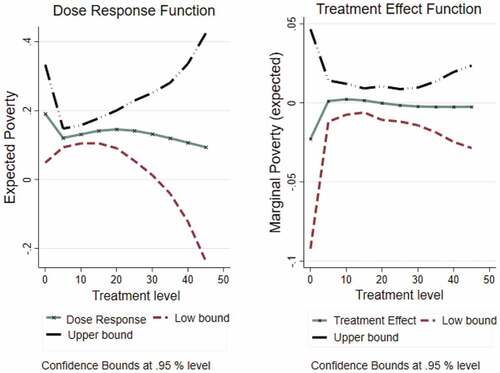
The estimated derivative of this function, the treatment-effect function is even more informative as it shows the responses to poverty with each additional year of receiving remittances. The GPS estimates of this function imply that the marginal propensity of being poor goes down with each additional year of receiving remittances, in the period between 0 and five years of receiving remittances. After this point, the marginal propensity of poverty continues to decrease with each additional year of receiving remittances, but the decrease is gradual in time. Our dose-response function flattens out for treatment levels extending over 30 years of receiving remittances. It means that more extended periods of time of receiving remittances (longer than 30 years) do not add an additional poverty reduction effect. Last but not least, it should be noted that confidence intervals appear wider at longer treatment levels due to a smaller number of observations in those levels (thus higher standard errors). Wider confidence intervals understandably reflect greater uncertainty in the data (and in the predictions) for those treatment levels.

In order to validate our results, we estimate the dose-response function for a second outcome variable that is the remittance recipient households’ yearly income (per capita equivalized) (Figure 2). The procedure differs from the previous dose-response estimation only in the last stage. The potential outcome that is averaged over the treatment level now is the households’ yearly income instead of the conditional probability of being poor.

Figure 2. Dose-response function of expected annual income.

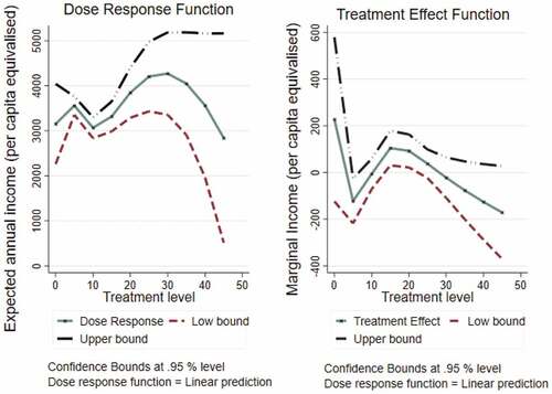
We expect a remittance dose-response on households’ yearly income to mirror the opposite of the response on poverty. If poverty decreases over the time-length a household receives remittances, the recipient households’ yearly income should be increasing. The obtained dose-response function on income indeed shows the expected behavior. As we see from the graph, there is a sharp increase in recipient households’ yearly income in the first five years of receiving remittances, followed by a decrease and then overall increase for households receiving remittances for more than ten years. The derivative of the dose-response confirms that the marginal propensity to “earn” out of remittances income increases sharply in the first five years. The overall response of income to the time-length of receiving remittances is positive.

Conclusion

For the first time in this field, this paper uses the dose-response estimation function to capture the impact of the time length of receiving remittances on the conditional probability of a household falling below a certain poverty threshold. We apply matching techniques and the dose response estimation to a dataset from Kosovo. The country ranks fourth among the top ten remittance-dependent European and Central Asian transition economies. Kosovo, like many other countries in the region, is strongly affected by migration and remittances, but widely under-researched in the discourse on development and welfare effects of remittances.

Our analysis contributes important empirical results on migration-dependent societies in two directions. First, our analysis confirmed that migration helps soothing poverty. In a counterfactual scenario, which reflects a situation in which migration is not possible, a higher percentage of households in Kosovo fell below a given poverty threshold, in particular in rural regions. Hence, migration was beneficial for those engaging in it by significantly raising migrant households’ yearly income vis-à-vis the non-migrant households. Although migration had a slightly un-equalizing effect on income, overall, an increase in social welfare is to be expected.

Second, the paper offers a promising methodological approach and empirical evidence with regard to the relationship between poverty (or the probability of being poor) and the time length a household received remittances. With an innovative method, which has not been applied before in migration research, we capture for the first time non-monotonic responses of remittances on recipient households’ probability to fall below a certain poverty line in a cross-sectional research design. While we find that remittances have a positive, poverty reducing effect over time, the effect is strongest in the first five years a household is exposed to remittances. Hence, the decreasing poverty effect of remittances may be most relevant in the short run. In the very long run, the effects of remittances flatten-out, thus suggesting that receipt of remittances impacts household poverty to a lesser degree. A standard PSM approach neglects the impact of the length of receiving remittances and would, thus, assign the same poverty-reducing effect of remittances to all households.

Our findings have important welfare policy implications for Kosovo and similar remittances-dependent transition economies by stressing the positive welfare impact of remittances. However, since dynamic effects seem to unfold primarily in the short term, longer-term effects of remittances should receive more attention of both researchers and policy makers.

Disclosure statement

No potential conflict of interest was reported by the authors.

Notes

1. Endogeneity is evident in the case when the existence of specific household characteristics (at times unobservable) which influence the decision to participate in migration, our independent variable whose impact we are trying to measure, simultaneously affect the outcome variable of interest. Endogeneity will almost certainly violate the OLS assumption of unconfoundedness, leading to biased estimates. Selection bias refers to the fact that migrant and non-migrant households differ inherently across some socio-economic characteristic, making the imputations of the outcomes of one group to the other, without a balanced matching, extremely problematic. Reverse causality happens when the outcome variable influences the independent variable, rather than the other way around. Omitted variable bias, also known as hidden bias, occurs when key variables that impact the outcome variable cannot be accounted for in the estimations because they are unobservable.

2. Propensity score matching relies on two assumptions, the Ignorable Treatment Assignment Assumption and the Stable Unit-Treatment Value Assumption. The Ignorable Treatment Assignment Assumption, also known as the Common Independence Assumption (CIA) maintains that conditional on a set of covariates X, the outcomes of treatment and non-treatment conditions are independent of the treatment status (Rosenbaum and Rubin 1983). In case a violation of the ignorable treatment assignment assumption is suspected, then a sensitivity analysis aiming at measuring the extent of the biases is desirable.

3. GPS relies on the assumption of weak unconfoundedness, which requires only pairwise independence of assignment into treatment with each of the potential outcomes. Based on this assumption, Imbens (2000) derive the proof of weak unconfounded assignment into treatment. It maintains that, given the GPS, assignment of each unit into treatment is weakly unconfounded for a set of pretreatment variables X. Given a weakly confounded assignment into treatment for a set of pretreatment variables X, the use of the GPS removes any biases that arise from differences in observed covariates.

4. The variable, which measures the length of time a household has been receiving remittances, does not follow a normal distribution. The assumption of normality of treatment is not crucial and it is possible to assume other distributions and estimate the GPS with methods such as maximum likelihood regression (Kluve et al. 2012).

5. While there no specific rule on the choice of the cutoff points and the number of intervals, it is advisable to divide the sample into a few groups of approximately equal size using the sample distribution of the treatment variable. In addition, any other user-specified rule that makes sense may be utilized (Guo and Fraser 2010).

6. The baseline model for the estimation of GPS at a given treatment level and observed covariates uses a maximum likelihood estimator. The use of an ordinary least squares regression, OLS, is deemed problematic because the model assumes constant variances of the error terms, when in practice, the variances of the error terms differ from one treatment level to the other. In presence of heteroskedasticity, the estimated standard errors of the OLS coefficients are wrong and the confidence intervals are not valid.

7. We used two questions from KRHS 2011 to identify migrant households. First, “Do you have any family members that live outside of Kosovo” is used as a primary identification question by a yes and no answer. Second, the follow up question “if yes, could you give us some information of these family members” was used to re-categorize those households which had provided detailed information on migrant family members, even if initially in question 26 they had indicated a no answer. This meant re-categorization as migrant households for a small number of households (N = 16).

8. We identify remittance recipients as those households that have received in-cash and in-kind contributions from international migrants in the year preceding the survey, excluding migrants’ visiting expenses.

9. The dependency ratio measures the ratio of dependent household members (those not of working age) by the number of those who are of working age.

10. “Other income” includes domestic remittances, pensions, rental income, social assistance and humanitarian aid, students’ scholarships and incomes unspecified by the respondents of the survey.

11. A number of papers however find that migrant households spend less on food and housing expenses and more for consumer durables, health and other types of investments vis-à-vis non-migrant households (see for instance Taylor and Mora 2006).

12. SWF = μ * (1-G), where μ is the average (mean) income and G is the Gini coefficient estimated for the entire sample.

13. The treatment variable varies from a minimum of 1 year to 43 years and it is constructed using question 30 in KRHS 2011, which asks, “When did you start receiving money from abroad?” and records as answer the year the household began receiving remittances.

Appendix

A. Figure Appendix

Figure A1. Densities of propensity scores before and after matching.

Figure A2.

Visual inspection of overlap condition.

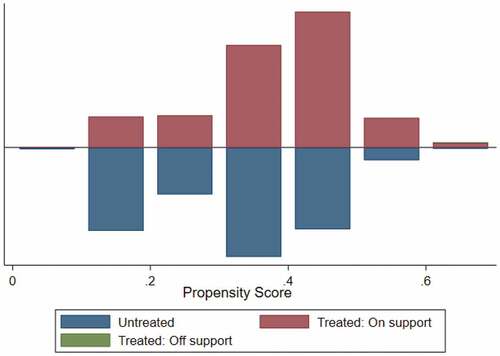
Figure A3.

Standardized percentage bias before and after matching.

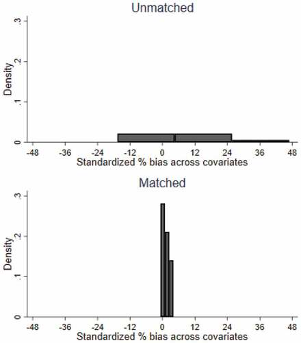
Figure A4.

Standardized percentage bias before and after matching.

B. Table Appendix

Table A1. Descriptive statistics of variables in the PSM logit model.

Independent variables		Mean/percentage share (for dummies)	Std.Dev.
agehhh	Age of household head	48.02	13.09
agesq	Squared age of household head	2477.23	1334.11
genderhh	Gender of household head (binary variable 1 = Male)	87%	–
pensioner	Household head is a pensioner (binary variable 1 = Pensioner)	7%	–
sharefemale	Share of female household members	47.62	0.17
munrem2011	Average shares of remittances for migrant households at municipality level in 2011	22.50	14.54
Albanian	Ethnicity is Albanian	75%	–
Prishtina	Region is Prishtina	23.09%	–
Prizren	Region is Prizren	18.43%	–
Peja	Region is Peja	14.24%	–

Source: Own calculation based on KRHS 2011 data.

N = 8,0000.

Table A2.

PSM logit results -psmatch2.

Independent variables	Coefficient	Std. Err.	z	P>|z|	95% Confidence Interval
agehhh	−0.02	0.01	−2.05	0.040	−0.05	0.00
agesq	0.00	0.00	3.08	0.002	0.00	0.00
genderhh	−0.16	0.07	−2.11	0.035	−0.30	−0.01
pensioner	0.20	0.11	1.90	0.057	−0.01	0.41
sharefemale	0.00	0.00	2.14	0.033	0.00	0.01
munrem2011	0.00	0.00	0.60	0.547	0.00	0.00
Albanian	1.17	0.07	17.62	0.000	1.04	1.30
Pristina	−0.56	0.07	−8.24	0.000	−0.69	−0.42
Prizren	−0.42	0.07	−6.01	0.000	−0.56	−0.29
Peja	−0.25	0.07	−3.42	0.001	−0.39	−0.11
_cons	−1.16	0.31	−3.78	0.000	−1.75	−0.56

Source: Own calculation based on KRHS 2011 data.

Note: N = 8,000.

LR chi2(9) = 545.23.

Prob > chi2 = 0.000.

Pseudo R2 = 0.053.

psmatch2 treatment assignment.

7, 988 on support, thereof 2,711 treated, 5,277 untreated.

Table A3.

Testing the balance of covariates and absolute bias reduction.

		Mean				t-test
Variable		Treated	Control	%bias	% reduction in bias	t	p > t
agehhh	Unmatched	49.80	47.11	20.4		8.76	0.000
	Matched	49.80	49.64	1.2	94.1	0.44	0.657
agesq	Unmatched	2666.50	2379.90	21.2		9.14	0.000
	Matched	2662.20	2632.20	2.2	89.5	0.80	0.425
genderhh	Unmatched	0.84	0.89	−12.4		−5.35	0.000
	Matched	0.84	0.85	−0.6	94.8	−0.23	0.822
pensioner	Unmatched	0.09	0.05	13.4		5.91	0.000
	Matched	0.09	0.08	4.0	70.1	1.38	0.167
sharefemale	Unmatched	48.60	47.12	8.7		3.67	0.000
	Matched	48.54	48.44	0.6	93.3	0.22	0.828
munrem2011	Unmatched	308.89	292.76	9.2		3.79	0.000
	Matched	309.04	302.54	3.7	59.7	1.49	0.135
Albanian	Unmatched	0.87	0.69	46.8		18.87	0.000
	Matched	0.87	0.87	1.1	97.7	0.49	0.625
Prishtina	Unmatched	0.19	0.25	−16.7		−6.94	0.000
	Matched	0.19	0.19	−0.7	95.7	−0.28	0.781
Prizren	Unmatched	0.17	0.19	−6.2		−2.62	0.009
	Matched	0.17	0.17	0.2	96.9	0.07	0.942
Peja	Unmatched	0.15	0.14	2.7		1.15	0.249
	Matched	0.15	0.14	1.9	30.3	0.69	0.488

Source: Own calculation based on KRHS 2011 data.

Table A4.

R2 of raw and matched model.

Sample	Pseudo R2	LR chi2	p> chi2	Mean bias	Median bias
Raw	0.053	539.58	0.000	15.3	12.4
Matched	0.001	5.01	0.833	1.7	1.1

Source: Own calculation based on KRHS 2011 data.

Table A5.

Rosenbaum bounds test for sensitivity.

Gamma	sig+	sig-	t-hat+	t-hat-	CI+	CI-
1	0	0	616.035	616.035	533.697	698.81
1.05	0	0	569.921	662.54	488.134	745.774
1.1	0	0	526.092	706.667	444.843	791.828
1.15	0	0	484.524	749.725	403.294	836.1
1.2	0	0	445.128	791.594	364.02	878.667
1.25	0	0	407.067	832.116	326.224	919.816
1.3	0	0	371.035	871.272	290.404	959.965
1.35	5.60E-16	0	336.538	908.696	256.138	998.901
1.4	2.50E-13	0	303.226	945.341	222.857	1036.6
1.45	5.00E-11	0	271.574	981.143	190.794	1073.25
1.5	4.80E-09	0	240.87	1016.05	160	1109.14
1.55	2.40E-07	0	211.201	1050	130.021	1143.96
1.6	6.80E-06	0	182.529	1082.95	100.922	1178.56
1.65	0.000112	0	154.783	1115.24	73.2592	1212
1.7	0.001136	0	127.917	1146.47	46.1538	1244.8
1.75	0.007491	0	101.584	1177.72	20	1277.14
1.8	0.03353	0	76.6421	1207.84	−5.41358	1308.57
1.85	0.106278	0	52.0953	1237.83	−30.0866	1339.23
1.9	0.248982	0	28.2052	1266.67	−54.5413	1369.24
1.95	0.450771	0	5.15147	1295.43	−78.0337	1399.33
2	0.661376	0	−17.381	1323.33	−100.879	1428.33

Source: Own calculation based on KRHS 2011 data.

Note: gamma – log odds of differential assignment due to unobserved factors

sig+ – upper bound significance level

sig- – lower bound significance level

t-hat+ – upper bound Hodges-Lehmann point estimate

t-hat- – lower bound Hodges-Lehmann point estimate

CI+ – upper bound confidence interval (α = .95)

CI- – lower bound confidence interval (α = .95)

Table A6.

Distribution of treatment intervals.

	Number of Households	Percentage (%)
Years of receiving remittances
Treatment Interval 1 (from 1 year to 5 years)	624	35.80
Treatment Interval 2 (from 6 years to 11 years)	730	41.88
Treatment Interval 3 (from 12 years to 43 years)	389	22.32
Total	1,743	100

Source: Own calculation based on KRHS 2011 data.

Table A7.

ML regression results to predict GPS.

Independent variables	Coef.	Std. Err.	z	P > z	95% Confidence Interval
Equation 1(1) $Y_i=D_i{Y}_{1i}+(1-D_i)Y_{0i}$(1)
Albanian	−0.05	0.10	−0.45	0.65	−0.24	0.15
Serb	−0.19	0.15	−1.31	0.19	−0.48	0.09
agehhh	0.00	0.00	1.82	0.07	0.00	0.01
genderhh	0.04	0.07	0.59	0.56	−0.09	0.17
educyhh	0.00	0.01	0.27	0.79	−0.01	0.02
married	−0.15	0.07	−2.15	0.03	−0.28	−0.01
familysize	0.04	0.01	3.27	0.00	0.02	0.07
depratio	0.00	0.00	4.34	0.00	0.00	0.00
employed	0.03	0.05	0.52	0.60	−0.07	0.13
Pristina	−0.46	0.06	−7.47	0.00	−0.58	−0.34
Mitrovica	−0.03	0.07	−0.38	0.70	−0.17	0.11
Gjilan	−0.13	0.07	−1.73	0.08	−0.27	0.02
Peja	0.01	0.07	0.08	0.94	−0.12	0.13
Ferizaj	−0.07	0.08	−0.88	0.38	−0.22	0.08
_cons	1.61	0.19	8.69	0.00	1.25	1.98
Equation 2(2) $R=r\left(T\mathit{,}X\right)$(2)
_cons	0.80	0.01	54.26	0.00	0.77	0.82

Source: Own calculation based on KRHS 2011 data.

The log transformation of the treatment variable is used; N = 1,472; Wald chi2(14) = 117.70; Prob > chi2 = 0.00

Table A8.

Covariate balance given the GPS.

	Adjusted for GPS
	Treatment Interval 1 [1,5]		Treatment Interval 2 [6,11]		Treatment Interval 3 [12,43]
Variable	Mean Difference	t-value	Mean Difference	t-value	Mean Difference	t-value
Albanian	0.018	1.430	−0.029	−2.345	0.030	1.867
Serb	−0.013	−1.516	0.015	1.659	−0.007	−0.551
agehhh	0.141	0.259	0.247	0.473	−0.509	−0.773
genderhh	−0.005	−0.288	0.010	0.625	−0.008	−0.408
educyhh	0.101	0.714	−0.233	−1.740	0.189	1.128
married	−0.004	−0.272	0.024	1.685	−0.025	−1.425
familysize	−0.033	−0.496	0.143	2.259	−0.074	−0.963
depratio	1.936	0.741	1.504	0.590	−4.028	−1.483
employed	0.006	0.290	−0.020	−0.948	0.038	1.432
Pristina	0.010	1.045	0.003	0.264	0.015	0.901
Mitrovica	−0.005	−0.284	0.030	2.039	−0.043	−2.341
Gjilan	−0.021	−1.462	0.025	1.791	−0.030	−1.673
Peja	−0.002	−0.110	0.016	1.034	−0.013	−0.683
Ferizaj	−0.008	−0.583	−0.003	−0.214	0.005	0.270

Source: Own calculation based on KRHS 2011 data.

Mean difference prior and after matching on GPS; t-statistics for equality of means.

Table A9.

Estimated ML coefficients given treatment variable and GPS.

Outcome variable: Conditional probability of being poor	Maximum Likelihood Coefficients	Standard Errors
Treatment	−0.010	0.072
Treatment_sq	0.000	0.002
pscore	−1.684	2.148
pscore_sq	0.920	2.116
treatment*pscore	0.046	0.090
_cons	−1.376	0.487

Source: Own calculation based on KRHS 2011 data.

Table A10.

Estimated OLS coefficients given treatment variable and GPS.

Outcome variable: Per capita equivalised income (in Euro)	OLS Coefficients	Standard Errors
Treatment	171.35	64.69
treatment_sq	−3.88	1.88
pscore	947.90	1991.54
pscore_sq	355.75	1931.07
treatment*pscore	−330.24	81.56
_cons	3110.20	468.26

Source: Own calculation based on KRHS 2011 data.

References

- Acosta, P., C. Calderón, P. Fajnzylber, and H. Lopez. 2008. “What Is the Impact of International Remittances on Poverty and Inequality in Latin America?” World Development 36 (1):89–114. doi:10.1016/j.worlddev.2007.02.016.
- Adams, R. 1989. “Worker Remittances and Inequality in Rural Egypt.” Economic Development and Cultural Change 38 (1):45–71. doi:10.1086/451775.
- Adams, R. 2006. “Remittances and Poverty in Ghana.” World Bank Policy Research Working Paper 3838, World Bank, Washington.
- Adams, R. 2011. “Evaluating the Economic Impact of International Remittances on Developing Countries Using Household Surveys: A Literature Review.” Journal of Development Studies 47 (6):809–28. doi:10.1080/00220388.2011.563299.
- Adams, R., and J. Page. 2005. “Do International Migration and Remittances Reduce Poverty in Developing Countries?” World Development 38 (11):1645–69. doi:10.1016/j.worlddev.2005.05.004.
- Alishani, A., and A. Nushi. 2012. “Migration and Development: The Effects of Remittances on Education and Health of Family Members Left behind for the Case of Kosovo.” Analytical Journal 5 (1):42–58.
- Amare, M., and L. Hohfeld. 2016. “Poverty Transition in Rural Vietnam: The Role of Migration and Remittances.” Journal of Development Studies 52 (10):1463–78. doi:10.1080/00220388.2016.1139696.
- Aslihan, A., and J. E. Taylor. 2012. “Transforming Rural Economies: Migration, Income Generation and Inequality in Rural Mexico.” Journal of Development Studies 48 (8):1156–76. doi:10.1080/00220388.2012.682985.
- Austin, P. C. 2014. “A Comparison of 12 Algorithms for Matching on the Propensity Score.” Statistics in Medicine 33 (6):1057–69. doi:10.1002/sim.6004.
- Barham, B., and S. Boucher. 1998. “Migration Remittances and Inequality: Estimating the Net Effects of Migration on Income Distribution.” Journal of Development Economics 55:307–31. doi: 10.1016/S0304-3878(98)90038-4.
- Bia, M., and A. Mattei. 2008. “A Stata Package for the Estimation of the Dose–response Function through Adjustment for the Generalized Propensity Score.” The Stata Journal 8 (3):354–73. doi:10.1177/1536867X0800800303.
- Citina, I., and I. Love. 2017. “Re-evaluating Microfinance: Evidence from Propensity Score Matching.” The World Bank Economic Review 33 (1):95–115. doi:10.1093/wber/lhw069.
- Coudouel, A., J. S. Hentschel, and Q. T. Wodon. 2002. “Poverty Measurement and Analysis.” In A Sourcebook for Poverty Reduction Strategies, 29-74, edited by J. Klugman. Washington, DC: World Bank.
- de Brauw, A., V. Mueller, and T. Woldehanna. 2018. “Does Internal Migration Improve Overall Well-Being in Ethiopia?” Journal of African Economies 27 (3):347–65. doi:10.1093/jae/ejx026.
- Duval, L., and F.-C. Wolff. 2015. “Ethnicity and Remittances.” Journal of Comparative Economics 43:334–49. doi: 10.1016/j.jce.2014.09.001.
- Feldman, S., and P. J. Leones. 1998. “Nonfarm Activity and Rural Household Income: Evidence from Philippine Microdata.” Economic Development and Cultural Change 46 (4):789–806. doi:10.1086/452374.
- Gang, N. Ira, K. Gatskova, J. Landon-Lane, and M.-S. Yun. 2018. “Vulnerability to Poverty: Tajikistan during and after the Global Financial Crisis.” Social Indicators Research 138 (3):925–51. doi:10.1007/s11205-017-1689-y.
- Guo, S., and M. Fraser. 2010. Propensity Score Analysis: Statistical Methods and Applications. Los Angeles: Sage Publications.
- Ham, J. C., X. Li, and P. B. Reagan. 2011. “Matching and Semi-parametric IV Estimation, a Distance-based Measure of Migration, and the Wages of Young Men.” Journal of Econometrics 161 (2):208–27. doi:10.1016/j.jeconom.2010.12.004.
- Heinrich, C., A. Maffioli, and G. Vázquez. 2010. A Primer for Applying Propensity-Score Matching Impact-Evaluation Guidelines. Washington DC, USA: Office of Strategic Planning and Development Effectiveness, Inter-American Development Bank.
- Hirano, K., and G. W. Imbens. 2004. “The Propensity Score with Continuous Treatment.” In Applied Bayesian Modeling and Causal Inference from Incomplete-Data Perspectives, 73-84, edited by A. Gelman and X.-L. Meng. Chichester: John Wiley.
- Imbens, G. W. 2000. “The Role of the Propensity Score in Estimating Dose-Response Functions.” Biometrika 87 (3):706–10. doi:10.1093/biomet/87.3.706.
- IMF. 2018. “Republic of Kosovo: Selected Issues.” IMF Country Reports (18/31 ed.), International Monetary Fund, Washington DC.
- Jimenez-Soto, E. V., and R. P. C. Brown. 2012. “Assessing the Poverty Impacts of Migrants’ Remittances Using Propensity Score Matching: The Case of Tonga.” Economic Record 88 (282):425–39. doi:10.1111/j.1475-4932.2012.00824.x.
- KAS. 2013. Consumption Poverty in the Republic of Kosovo in 2011. Prishtina: [KAS] Kosovo Agency of Statistics, The World Bank.
- Kimhi, A. 2010. “International Remittances, Domestic Remittances, and Income Inequality in the Dominican Repulic.” Accessed 18 April 2016. http://departments.agri.huji.ac.il/economics/indexe.html.
- Kluve, J., H. Schneider, A. Uhlendorff, and Z. Zhao. 2012. “Evaluating Continuous Training Programmes by Using the Generalized Propensity Score.” Statistics in Society Series A 175 (2):587–617. doi:10.1111/j.1467-985X.2011.01000.x.
- Lerman, I., and S. Yitzhaki. 1985. “Income Inequality Effects by Income Source: A New Approach and Applications to the United States.” The Review of Economics and Statistics 67 (1):151–56. doi:10.2307/1928447.
- McKenzie, D., and M. J. Sasin. 2007. “Migration, Remittances, Poverty, and Human Capital.” World Bank Policy Research Working Paper 4272, World Bank, Washington DC. .
- Möllers, J., and W. Meyer. 2014. “The Effects of Migration on Poverty and Inequality in Rural Kosovo.” IZA Journal of Labor & Development 3 (16). doi:10.1186/2193-9020-1183-1116.
- Oberai, A. S., and H. K. M. Singh. 1983. Causes and Consequences of International Migration: A Study in the Indian Punjab. New Delhi: Oxford University Press.
- OECD. 2018. What are Equivalence Scales? Paris: Organisation for Economic Co-operation and Development. http://www.oecd.org/eco/growth/OECD-Note-EquivalenceScales.pdf.
- Ravallion, M., S. Chen, and P. Sangraula 2008. “Dollar a Day Revisited.” Policy Research Working Paper 4620, The World Bank, Development Research Group, Washington DC, USA.
- Rosenbaum, R. Paul, and B. Donald Rubin. 1983. “The Central Role of Propensity Score in Observational Studies for Causal Effects.” Biometrika (70):41–55. doi:10.1093/biomet/70.1.41.
- Shen, I.-L., F. Docquier, and H. Rapoport. 2010. “Remittances and Inequality: A Dynamic Migration Model.” The Journal of Economic Inequality 8 (2):197–220. doi:10.1007/s10888-009-9110-y.
- Stark, O., J. E. Taylor, and S. Yitzhaki. 1986. “Remittances and Inequality.” The Economic Journal 96(No (383)):722–40. doi:10.2307/2232987.
- Stark, O., and S. Yitzhaki. 1982. “Migration, Growth, Distribution and Welfare.” Economics Letters 10 (1982):243–49. doi:10.1016/0165-1765(82)90061-1.
- Taylor, J. E. 1992. “Remittances and Inequality Reconsidered: Direct, Indirect, and Intertemporal Effects.” Journal of Policy Modeling 14 (2):187–208. doi:10.1016/0161-8938(92)90008-Z.
- Taylor, J. E., and J. Mora 2006. “Does Migration Reshape Expenditures in Rural Households? Evidence from Mexico.” World Bank Policy Research Working Paper 3842, World Bank, Washington DC.
- Taylor, J. E., J. Mora, R. Adams, and A. Feldman-Lopez 2005. “Remittances, Inequality and Poverty: Evidence from Rural Mexico.” ARE Working Papers No. 05-003, University of California, Davis.
- Taylor, J. E., S. Rozelle, and A. de Brauw. 2003. “Migration and Incomes in Source Communities: A New Economics of Migration Perspective from China.” Economic Development and Cultural Change 52 (1):75–101. doi:10.1086/380135.
- UN. 2015. Transforming Our World: The 2030 Agenda for Sustainable Development. Resolution Adopted by the General Assembly on 25 September 2015. New York, NY: United Nations (UN). https://sustainabledevelopment.un.org/post2015/transformingourworld.
- World Bank. 2011. “Migration and Economic Development in Kosovo.” Report No. 60590 – XK, World Bank, Washington DC.
- World Bank. 2017. “World Bank Open Data.” Accessed 15 June 2019. https://data.worldbank.org/indicator/NY.GDP.PCAP.CD?locations=XK&view=chart.
- World Bank. 2018. “Migration and Remittances: Recent Development and Outlook.” In World Bank Migration and Development Brief, 22:1-21. Washington DC, USA: World Bank Group.
- Yang, D., and C. Martinez. 2006. “Remittances and Poverty in Migrants Home Areas: Evidence from the Philippines.” In International Migration, Remittances and the Brain Drain, 81-121, edited by C. Ozden and M. Schiff. Washington, DC: World Bank.