Avoiding momentum crashes using stochastic mean-CVaR optimization with time-varying risk aversion

Abstract

In occasions called momentum crashes, the usually effective cross-sectional momentum strategy for financial asset allocation produces drastically negative returns. We develop a stochastic mean-risk optimization model featuring CVaR to control the risk, dynamically adjusted CVaR tail probability and objective function weight, and return scenarios generated by hybrid moment-matching. In a 95-year backtest, portfolios rebalanced by our method provide higher returns and lower risk than those rebalanced by a cross-sectional momentum heuristic, while avoiding momentum crashes.

1. Introduction

Momentum in finance is an empirical observation that trends in asset returns persist over the short term. The existence of momentum is a market anomaly as it contradicts the efficient market hypothesis that past returns cannot determine the current return. Investors exploit this return predictability of momentum to construct trading strategies that take a long position (buy in anticipation of an increase in value) in upward trending assets and a short position (sell first with the plan to buy later at a lower price) in downward trending assets with the expectation that their momentum will extend the trends.

The cross-sectional momentum trading strategy, that forms portfolios by cross-sectional ranking, is the most typical and frequently-used momentum trading strategy. It originates from the work of Jegadeesh and Titman (1993), who rank the cross-section of stocks according to the three- to twelve-month past returns to identify winners (stocks that have performed well) and losers (stocks that have performed poorly), buy past winners and short past losers, and hold these positions for up to twelve months. They find that over the 1965 to 1989 period, past losers continued to perform badly and past winners continued to perform well during these holding periods, indicating that cross-sectional momentum exists and no return reversals occur in the short term. In this paper, we refer to portfolios composed of past winners and/or past losers as momentum portfolios.

Evidence supporting cross-sectional momentum is plentiful. Jegadeesh and Titman (1993) find that the momentum strategy can gain as much as 1.49% per month in the US stock market. Furthermore, momentum is not only an anomaly in the US stock market, but also observed in European equities, emerging markets, country indices, industry portfolios, currencies, commodities, and across asset classes (Asness et al., 1997; Grinblatt & Titman, 1993; Grobys et al., 2018; Okunev & White, 2003). Compared to the factors (market, value, and size) in the classic Fama and French three-factor asset pricing model, cross-sectional momentum offers the highest Sharpe ratio (Barroso & Santa-Clara, 2015).

However, the remarkable performance of momentum strategies comes with large crashes occasionally. Daniel and Moskowitz (2016) show that the cross-sectional momentum strategy would have produced infrequent and persistent negative returns in the US stock market in 1932 and 2009, where the return derived by the strategy would have been −91.59% over two months and −73.42% over three months, respectively. Recovering from the negative impact of these crashes would have taken decades. Daniel and Moskowitz (2016) find that these two crashes both happened when the market rebounded following a severe bear market. They conclude that the reason behind this phenomenon is the asymmetric behavior of past winner and loser portfolios: the return of past losers grows rapidly when the market is volatile and the market return increases after a bear market, making the past losers behave like a call option on the market; while past winner portfolios do not show any similar behavior during the same period. This asymmetric behavior causes a reversal in the relationship between past losers and past winners in the recovery phase and, thus, leads to a huge loss for the momentum strategy that shorts the past losers.

The occurrence of momentum crashes is due primarily to the uncertainty of the stock market, especially concerning the time when the bear market ends and past losers stop being losers. In this paper, to improve on the performance of the cross-sectional momentum strategy and avoid momentum crashes, we explore alternative ways to allocate investment between a risk-free asset and the two momentum portfolios: (1) control the risk of momentum portfolios, (2) exploit time-varying risk aversion to adjust the momentum trading strategy according to the stock market states, and (3) simulate momentum portfolio returns in a way that comprehensively accounts for the possible returns in the next period.

To manage the risk of the investment strategies, the risk measure must be selected. Barroso and Santa-Clara (2015) and Daniel and Moskowitz (2016) both quantify the risk of momentum portfolios in terms of volatility (variance). Inspired by the risk parity approaches (Asness et al., 2012), Barroso and Santa-Clara (2015) scale the winner-minus-loser (WML) portfolio return by its realized volatility of past six-month returns to control the investment risk of the cross-sectional momentum strategy. Daniel and Moskowitz (2016) maximize the Sharpe ratio of the WML portfolio, which turns to be a variant of the traditional Markowitz mean-variance approach (Markowitz, 1952). Volatility and variance quantify risk in terms of both upside gains and downside losses and, thus, cannot distinguish the direction of investment movement. However, investors worry about the loss only. In addition, researchers have found that higher moments, such as skewness and kurtosis, are non-negligible in asset allocation when the asset returns are not normally distributed. Therefore, a downside risk measure, capable of being expressed as a function of skewness and kurtosis for non-normal investment returns and assessing the extent of losses only (Xiong & Idzorek, 2011), is more suitable to reduce the risk of momentum investing. By far, value at risk (VaR) and conditional value-at-risk (CVaR) are the two most commonly-used downside risk measures in finance (Banihashemi & Navidi, 2017; Benati & Conde, 2022; Guo et al., 2019; Kim & Park, 2021; Kim et al., 2012; Sharifi & Kwon, 2018). VaR estimates the maximum loss that could occur over a given period with a specified confidence level. CVaR is defined as the conditional expectation of portfolio losses beyond a prespecified percentile of the distribution of the loss (Rockafellar & Uryasev, 2000). Although both VaR and CVaR are superior to variance for asymmetric asset return distributions, there are two reasons for the preference in portfolio and risk management of CVaR relative to VaR. First, CVaR takes into account not only the probability but also the size of the loss (Rockafellar & Uryasev, 2000). Second, Pflug (2000) proves that CVaR satisfies the properties for a coherent risk measure while VaR fails due to the violation of the sub-additivity property, which posits that diversification reduces risk. More recently, Ahmadi-Javid (2012) proposes a new risk measure, entropic value-at-risk (EVaR), which uses the Chernoff inequality to create an upper bound for the CVaR and is proven to be coherent. Compared to CVaR, EVaR has stronger monotonicity and is more computationally efficient when solving large-scale optimization problems due to the number of variables and constraints of the EVaR formulation being independent of the sample size (Ahmadi-Javid & Fallah-Tafti, 2019). However, EVaR is more risk-averse at the same confidence level than CVaR; that is, the incorporation of EVaR will result in allocating more resources to avoid risk, which may not be favored by investors who want to allocate the least amount of resources. This property makes EVaR less attractive than CVaR.

Having selected CVaR as the risk measure, a mean-CVaR stochastic program with time-varying risk aversion is developed to balance the tradeoff between investment risk and reward. Stochastic programming provides a modeling framework for decision making under uncertainty. It is well suited for portfolio management as investment decisions have to be made before the return information is revealed. Numerous applications of stochastic programming to portfolio management have been studied in the past decades (Bergk et al., 2021; Cui et al., 2020; Guo & Ryan, 2021 2021a; Lim et al., 2011; Moazeni et al., 2016; Topaloglou et al., 2011). Motivated by the regime-switching model (Bae et al., 2014; Li et al., 2022), in this paper, we incorporate time-varying risk aversion to select portfolio weights that dynamically balance the tradeoff between expectation and CVaR of the return of the constructed portfolio according to various stock market conditions. As momentum crashes happen when the market is volatile, we explore three volatility-related measures, namely (1) estimated market volatility, (2) the ratio of estimated market return to estimated market volatility, and (3) the Chicago Board Options Exchange (CBOE) Volatility Index (VIX), to determine the tail probability in CVaR and the risk-aversion parameter in the mean-CVaR model.

One of the biggest advantages of stochastic programming is its flexibility in modeling uncertainty. In a stochastic program, the uncertainty of the input parameters is represented in terms of discretely distributed scenarios. The various approaches to generating scenarios in stochastic programs can be categorized into two classes depending on whether the distribution of the uncertain parameters is specified or not. When the distribution is specified, Monte Carlo simulation can be applied to generate scenarios by repeated random sampling from the specified distribution (Guo & Ryan, 2021; Ripley, 1987; Sharifi et al., 2016; Yu et al., 2003). On the other hand, when the joint distribution of the uncertain parameters is not specified, bootstrapping, which samples the historical data randomly with replacement, is a straightforward way to generate scenarios (Barro et al., 2019; Thomann, 2021; Zou et al., 2019). Although bootstrapping is easy to implement, it is unable to capture some inherent structure of stock returns. Høyland and Wallace (2001) propose a moment-matching method that consists of sequentially solving an optimization problem with the objective to minimize the distance between the statistical properties of scenarios and specified target values estimated on the basis of historical data. Høyland et al. (2003) propose a heuristic procedure to approximately implement the moment-matching method for the first four marginal moments and correlations. To approximate the unknown distribution of momentum portfolio returns, including the large kurtosis indicated by occasional momentum crashes, we employ a combination of heuristic and optimization moment-matching algorithms to generate scenarios of future returns of the momentum portfolios.

Upon generating scenarios, the next question arising in a backtesting environment is how well they match the observed data. The verification rank histogram, a recently-developed technique that compares sets of scenarios that would have been generated in the past with the corresponding observations, can be applied to evaluate the quality of scenarios. The mass transportation distance (MTD) rank histogram (Sar I et al., 2016) is one such verification rank histogram. The principle behind the rank histogram is that the set of reliable scenarios generated at a given time point and its corresponding observation can be regarded as random samples drawn from the same distribution. It evaluates the reliability of the scenarios according to the uniformity of the distribution of the rank of the scenarios-to-observation distance among corresponding distances from each scenario to the rest, augmented by the observation. Therefore, the rank of the distance between reliable scenarios and the observation should be equally likely to fall in any bin of the histogram, meaning that the rank histogram of reliable scenarios should have all bins at a very similar height.

Finally, we empirically analyze the performance of the mean-CVaR solutions with time-varying risk aversion in a historical backtest of monthly rebalancing. The stock universe consists of all stocks listed on NYSE, AMEX, and NASDAQ with the returns of the common shares. Using historical data from 1926 through 2020, we find that weights derived from our mean-CVaR model with time-varying risk aversion defined using volatility of market returns are robust to the number of months used to estimate market index return mean and volatility. For all such numbers of months tested, the resulting portfolio achieves higher excess returns, Sharpe ratio, and upside potential ratio, as well as lower maximum drawdown, than a heuristic solution corresponding to the cross-sectional momentum strategy. In addition, no drastic decline in cumulative returns occurs during the whole simulation horizon. An interesting finding is that no momentum crash would have occurred in 2020 when using either our mean-CVaR model or the cross-sectional momentum heuristic despite the steep decline in the stock market. During the two momentum crash periods, the cumulative returns achieved by rebalancing according to the mean-CVaR solutions held steady around the level of one, indicating that no huge loss is incurred when using this mean-CVaR model and, thus, the momentum crashes would have been avoided completely.

This paper’s contribution is a new trading strategy based on cross-sectional momentum, that successfully avoids the momentum crashes and is profitable in various states of the stock market. In this strategy, the investment risk is quantified by downside loss, the risk aversion is time-dependent to flexibly adjust the investment strategy according to the changing market conditions, and the uncertain momentum portfolio returns are well-represented by reliable scenarios that comprehensively account for the possibilities of the possible winner and loser returns that may occur in the next period. To the best of our knowledge, this is the first study to address the issue of momentum crashes using stochastic optimization.

The remainder of this paper is organized as follows. Section 2 lists the notations used throughout the whole paper, describes the construction of past winner and loser portfolios in the cross-sectional momentum strategy, and explains the reason to use returns of these two portfolios as random input parameters in Section 3, where a two-stage stochastic mean-CVaR optimization model with time-varying risk aversion is introduced. Section 4 illustrates a hybrid of heuristic and optimization moment-matching algorithms to generate scenarios of past winner and past loser portfolio returns and evaluates the reliability of the generation procedure. Section 5 describes the metrics used to evaluate the performance of the investment strategies. Section 6 presents the numerical experiments and analyzes the results. Section 7 finally concludes.

2. Notation and Preliminaries

This section lists the notations used in the whole paper, describes the construction of past winner and loser portfolios in the cross-sectional momentum strategy, and explains the reason to use returns of these two portfolios as random input parameters.

2.1. Notation

Notations used throughout this paper are defined as follows:

Sets and cardinalities:

• B   Set of candidate stocks in the stock market with cardinality $\left|B\right|$

• K   Number of look-back periods for identifying past winner and loser portfolios

• T   Number of periods in the simulation horizon

• W_t    Set of stocks in the past winner portfolio for period t, $W_t\subset B,t=1,\dots ,T$

• L_t   Set of stocks in the past loser portfolio for period t, $L_t\subset B,t=1,\dots ,T$

• J    Constant number of scenarios generated for each period t, $t=1,\dots ,T$

• M     Set of all specified statistical properties for scenario generation

• H   Number of periods used to estimate statistics in M

• P   Number of periods used to estimate mean of market returns for adjusting risk parameters

• G   Number of periods used to estimate volatility of market returns for adjusting risk parameters

• N   Number of periods in a year

Deterministic input data:

• $S_t^b$  Observed price of stock $b\in B$ at time $t=1,\dots ,T-1$

• $O_t^b$ Number of shares outstanding of stock $b\in B$ at time $t=1,\dots ,T-1$

• $r_t^b$  Observed rate of return for stock $b\in B$ in period $t=1,\dots ,T-1$

• $r_t^W$ Observed rate of return for the past winner portfolio in period $t=1,\dots ,T-1$

• $r_t^L$ Observed rate of return for the past loser portfolio in period $t=1,\dots ,T-1$

• r^t  Realized rate of return for the constructed portfolio in period t, which is an output in Section 3 and an input in Section 5, $t=1,\dots ,T$

• $r_t^f$  Risk-free rate of return in period $t=1,\dots ,T$

• i_t   Market index return rate in period $t=1,\dots ,T-1$

• $M_{\mathit{VALm},t}$ Specified value of statistical property $m\in M$ for period $t=1,\dots ,T$

• v_m Weight assigned to statistical property $m\in M$

Parameters for the portfolio optimization model for period t, $t=1,\dots ,T:$

• $R_t^W$   Random variable of the rate of return for the past winner portfolio in period t with scenarios $r_{t,j}^W,j=1,\dots ,J$

• $R_t^L$   Random variable of the rate of return for the past loser portfolio in period t with scenarios $r_{t,j}^L,j=1,\dots ,J$

• m_t   Market return estimated for period t

• σ_t   Market volatility estimated for period t

• A_t   Rank of σ_t among ${\sigma }_k,k=1,\dots ,t,$ sorted in increasing order

• B_t   Rank of $\frac{m_t}{{\sigma }_t}$ among $\frac{m_k}{{\sigma }_k},k=1,\dots ,t,$ sorted in decreasing order

• C_t   Rank of VIX at time t among values up to t sorted in increasing order

• λ_t   Risk-aversion parameter for period t, ${\lambda }_t\in [0,1]$

• α_t   Probability specified for CVaR to pertain to 100(1-α_t)% worst outcomes for period t, ${\alpha }_t\in [0,1]$

Decision variables in scenario generation procedure for period t, $t=1,\dots ,T:$

• $p_{t,j}$   Probability of the occurrence of scenario j, $j=1,\dots ,J$

• $r_{t,j}^W$   Return of the past winner portfolio in scenario j, $j=1,\dots ,J$

• $r_{t,j}^L$   Return of the past loser portfolio in scenario j, $j=1,\dots ,J$

Decision variables in the portfolio optimization model for period t, $t=1,\dots ,T:$

• $w_t^W$ Weight on the past winner portfolio

• $w_t^L$ Weight on the past loser portfolio

• $w_t^f$ Weight on the risk-free asset

• η_t α-quantile of the negative return rate of the constructed portfolio according to the scenarios generated for period t

• ${\nu }_{t,j}$ Deviation of the return rate of the constructed portfolio below η_t in scenario j as a non-negative simple recourse variable, $j=1,\dots ,J$

• $w_t^{W*}$ Optimal weight on the past winner portfolio

2.2. Past Winner and Past Loser Portfolios

In this paper, the past winner and loser portfolios, instead of the individual stocks, are used as the basis of the optimization model for two reasons. First, Daniel and Moskowitz (2016) conclude that momentum crashes occur because the winner-minus-loser (WML) portfolio behaves like shorting a call option on the market during the rebound from a bear market. However, this optionality is asymmetric as it is mainly associated with the past loser portfolios. The second reason is the concern about the computational cost when generating scenarios of returns and using them as inputs to the stochastic optimization model. Compared to generating scenarios of all stocks that constitute the past loser and winner portfolios at each time, generating scenarios for only past winner and loser returns is much faster to implement.

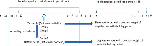
We rebalance our portfolio every period and the holding period is the interval between two rebalancing time points. Denote the beginning of period t as time t − 1 and its end as time t. To form the past winner and loser portfolios used in the cross-sectional momentum strategy proposed by Jegadeesh and Titman (1993), at time t − 1 we rank stocks based on their cumulative returns from K periods before to one period before the formation date (i.e. the $(t-K)$ to $(t-2)$-period return), ${\Pi }_{i=t-K}^{i=t-2}(1+r_i^b)-1,$ in ascending order. The one-period gap here is used to avoid short-term reversal, some of the bid-ask spread, price pressure, and lagged reaction effects mentioned in Lehmann (1990) and Jegadeesh and Titman (1993). Based on these rankings, the past winner portfolio for period t is constructed by value weighting the bottom decile stocks, denoted as W_t, and the past loser portfolio for period t is composed by value weighting the top decile stocks, represented by L_t. To obtain the value weight of stock b in W_t or L_t, the stock price, $S_{t-1}^b,$ and the number of shares outstanding, $O_{t-1}^b,$ of stock b at time t − 1 are used. More specifically, for $b\in W_t,$ the value weight in period t is (1) $$v_t^b=\frac{S_{t-1}^b{O}_{t-1}^b}{\sum _{a\in W_t}{S}_{t-1}^a{O}_{t-1}^a}$$(1)

Similarly, the value weight of $b\in L_t$ in period t is (2) $$v_t^b=\frac{S_{t-1}^b{O}_{t-1}^b}{\sum _{a\in L_t}{S}_{t-1}^a{O}_{t-1}^a}$$(2)

Consequently, the return rates of past winner and loser portfolios in period t, $r_t^W$ and $r_t^L,$ are the value-weighted average of returns in period t of the stocks composing the winner and loser portfolios in the look-back period, respectively: (3) $$r_t^W\equiv \sum _{b\in W_t}{v}_t^b{r}_t^b$$(3) and (4) $$r_t^L\equiv \sum _{b\in L_t}{v}_t^b{r}_t^b$$(4)

The construction of the cross-sectional momentum strategy is illustrated in Figure 1. This strategy has weight one on the past winner portfolio, negative one on the past loser portfolio, and zero on the risk-free asset. To avoid redundancy, we refer to the past winner and past loser portfolios simply as winner and loser portfolios, respectively, for the rest of the paper, unless otherwise noted.

Figure 1. Illustration of cross-sectional momentum strategy.

3. Stochastic Mean-CVaR Optimization Model with Time-Varying Risk Aversion

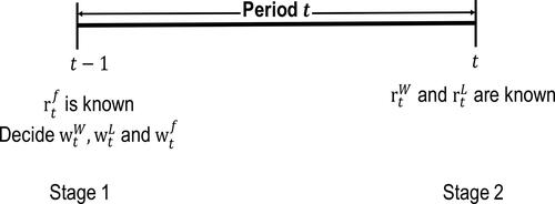
In this section, we introduce a two-stage stochastic optimization model to dynamically allocate funds between the cross-sectional momentum portfolio and a risk-free asset. At time t − 1, investors must determine the proportions of wealth, $w_t^W,w_t^L,$ and $w_t^f,$ to invest in the winner and loser portfolios and the risk-free asset, respectively, to maximize the total return and minimize the investment risk of the constructed portfolio in period t. However, the actual returns for the winners and the losers, $r_t^W$ and $r_t^L,$ in which we invest at time t − 1 will not be known until time t. This model is solved on a rolling basis. More specifically, we use the observation of the risk-free rate in period t and the scenarios for the cross-sectional momentum portfolio return at time t to rebalance the investment at time t − 1. After solving the model at time t − 1, the returns of the momentum portfolios in period t will be realized and stocks in loser and winner portfolios will be updated, according to which we can obtain new scenarios for the return rates of momentum portfolios in period t + 1. The new scenarios, along with the updated observation of the risk-free rate in period t + 1, are input to the optimization model to optimally rebalance at time t. This rebalancing process will be continued through period T. The decision point and information release schedule of each period are illustrated in Figure 2.

Figure 2. Timeline of period t.

3.1. Mean-CVaR Optimization Model

To balance the tradeoff between return and risk, Daniel and Moskowitz (2016) derive a rebalancing strategy to maximize the Sharpe ratio over the long term subject to a constraint on variance. However, the variance constraint considers gains and losses equally, which does not characterize the investors’ attitudes toward risk accurately when the distribution of the investment loss is not symmetric. As an alternative to variance, we consider a downside risk measure, conditional value-at-risk (CVaR) in each period. The CVaR of a loss random variable, Z, at a given probability, α, is defined as the conditional expectation of the loss of the portfolio exceeding or equal to value at risk, $\eta (\alpha ):$ (5) $${\text{CVaR}}_{\alpha }\left[Z\right]=\mathrm{E}\left[Z\right|Z\ge \eta (\alpha )]$$(5) where $\eta (\alpha )\equiv \min \left\{z|P(Z\le z)\ge \alpha ,\alpha \in [0,1]\right\}$ is the α-quantile of Z. Rockafellar and Uryasev (2002) further demonstrate that CVaR can be computed as follows: (6) $${\text{CVaR}}_{\alpha }\left[Z\right]=\eta (\alpha )+\frac{1}{1-\alpha }\mathrm{E}\left[{\left(Z-\eta (\alpha )\right)}_{+}\right]$$(6) where ${(Z-\eta (\alpha ))}_{+}\equiv \max (Z-\eta (\alpha ),0).$ By controlling CVaR, we can reduce the expected investment loss during the infrequent but devastating momentum crash periods and, thus, mitigate momentum crashes. In our model, Z represents the negative return of the optimized portfolio realized at time t. Therefore, the objective at time t − 1, to maximize the expected total portfolio return while minimizing the investment risk measured by CVaR, can be formulated as (7) $$\underset{{}_{w_t^W,w_t^L,w_t^f,{\eta }_t}}{\min }(1-{\lambda }_t)\mathrm{E}\left[-\left(R_t^W{w}_t^W+R_t^L{w}_t^L+r_t^f{w}_t^f\right)\right]+{\lambda }_t\left({\eta }_t+\frac{1}{1-{\alpha }_t}\mathrm{E}\left[{\left(-\left(R_t^W{w}_t^W+R_t^L{w}_t^L+r_t^f{w}_t^f\right)-{\eta }_t\right)}_{+}\right]\right)$$(7) where $R_t^W$ and $R_t^L$ are the random variables of the winner and loser returns, respectively, at time t. The risk-aversion coefficient λ_t represents how risk-averse the investors want the investment strategy to be: The larger the value of λ_t, the more conservative the strategy. Traditional mean-CVaR models (Chen et al., 2012; Cui et al., 2020; Lim et al., 2011)) use constant tail probability, $1-\alpha ,$ and risk-aversion parameter, λ. However, in reality, investors’ attitude toward risk or behavior in response to perceived risk may fluctuate over time due to the rapidly-shifting financial market. Hence, we extend the traditional mean-CVaR models by allowing α and λ to change over time.

Furthermore, when the joint distribution of $R_t^W$ and $R_t^L$ is approximated by a finite number of probabilistic scenarios, model (7) is transformed into a linear program (Rockafellar & Uryasev, 2000). Upon approximating the joint distribution of $R_t^W$ and $R_t^L$ by J scenarios ${\{(r_{t,j}^W,r_{t,j}^L)\}}_{j=1}^{j=J}$ with the joint probabilities ${\left\{p_{t,j}\right\}}_{j=1}^{j=J},$ the optimization model for period t is the linear program: (8) $$\underset{{}_{w_t^W,w_t^L,w_t^f,{\eta }_t,{\left\{{\nu }_{t,j}\right\}}_{j=1}^J}}{\min }(1-{\lambda }_t)\left[-\sum _{j=1}^J{p}_{t,j}(r_{t,j}^W{w}_t^W+r_{t,j}^L{w}_t^L)-r_t^f{w}_t^f\right]+{\lambda }_t\left({\eta }_t+\frac{1}{1-{\alpha }_t}\sum _{j=1}^J{p}_{t,j}{\nu }_{t,j}\right)$$(8) (9a) $$\mathrm{s}.\mathrm{t}.\hspace{1em}-1\le w_t^W\le 1,$$(9a) (9b) $$-1\le w_t^L\le 1,$$(9b) (9c) $$w_t^W+w_t^L=0,$$(9c) (9d) $$w_t^W+w_t^L+w_t^f=1$$(9d) (9e) $${\nu }_{t,j}\ge -p_{t,j}(r_{t,j}^W{w}_t^W+r_{t,j}^L{w}_t^L)-r_t^f{w}_t^f-{\eta }_t,j=1,\dots ,J$$(9e) (9f) $${\nu }_{t,j}\ge 0,j=1,\dots ,J$$(9f)

As shown in (8), the objective function takes a convex combination of mean and CVaR to achieve the goal of maximizing the expected overall return while minimizing CVaR at time t. Note that the cross-sectional momentum strategy (Jegadeesh & Titman, 1993) is to long winners and short losers, which can be expressed as $w_t^W\equiv 1$ and $w_t^L\equiv -1$ for $\forall t\in \{1,\dots ,T\}.$ To be consistent with the original momentum strategy, we allow short sale for the loser portfolios, represented by (9b). However, the setting of (9a) and (9b) is not exactly the same as the original momentum strategy because these two constraints not only allow us to follow the momentum strategy of shorting losers and longing winners but also grant the permission to long losers and short winners. Furthermore, the original momentum strategy for the investment in the winners and losers is zero-cost, which can be expressed as the sum of the weight of the loser and the weight of the winner must be zero, as presented in (9c). By forcing the investment in the momentum portfolios to be zero-cost and restricting the weights on the losers and winners to the interval $[-1,1],$ (9a)-(9c) include the original momentum strategy coupled with the risk-free asset as a feasible solution to this optimization model. Constraint (9d) enforces the total budget to invest in the winner and loser portfolios and the risk-free asset to equal the current wealth, which means the weights of all investment sum to one. Lastly, constraints (9e) and (9f) combine to compute the deviation of the weighted returns of the winner, the loser, and the risk-free asset below this value in scenario j as a non-negative simple recourse variable: ${\nu }_{t,j}={(-p_{t,j}(r_{t,j}^W{w}_t^W+r_{t,j}^L{w}_t^L)-r_t^f{w}_t^f-{\eta }_t)}_{+}.$

For each period t, the model (8) - (9f) can be reduced to the following form, suppressing the subscript t for clarity. (10) $$\underset{{}_{w^W,\eta ,{\left\{{\nu }_j\right\}}_{j=1}^J}}{\min }(1-\lambda )\left[-\sum _{j=1}^J{p}_j(r_j^W-r_j^L)w^W-r^f\right]+\lambda \left(\eta +\frac{1}{1-\alpha }\sum _{j=1}^J{p}_j{\nu }_j\right)$$(10) (11a) $$\mathrm{s}.\mathrm{t}.\hspace{1em}-1\le w^W\le 1,$$(11a) (11b) $${\nu }_j\ge -p_j(r_j^W-r_j^L)w^W-r^f-\eta ,j=1,\dots ,J$$(11b) (11c) $${\nu }_j\ge 0,j=1,\dots ,J$$(11c)

A simple structure for the optimal solution to the model (10) - (11c) can be derived in a manner similar to Proposition 1 in Guo and Ryan (2021a). Since CVaR is a coherent risk measure, the risk-free rate at each time is a deterministic constant and expectation is linear, we find the optimal weight to allocate to the past winner portfolios as follows. (12) $$w^{W*}=\{\begin{array}{cc}-1,\hfill & \text{ if }{c}^2(\lambda ,\alpha )>0\text{ and }{c}^1(\lambda ,\alpha )>-c^2(\lambda ,\alpha )\hfill \\ 0,\hfill & \text{ if }{c}^1(\lambda ,\alpha )\ge 0\text{ and }{c}^2(\lambda ,\alpha )\le 0\hfill \\ 1,\hfill & \text{ if }{c}^1(\lambda ,\alpha )<0\text{ and }{c}^2(\lambda ,\alpha )<-c^1(\lambda ,\alpha )\hfill \end{array}$$(12) where $c^1(\lambda ,\alpha )=(\lambda -1){\sum }_{j=1}^J{p}_j(r_j^w-r_j^l)+\lambda (\eta +\frac{1}{1-\alpha }{\left[-{\sum }_{j=1}^J{p}_j(r_j^w-r_j^l)-\eta \right]}_{+}),$ and $$c^2(\lambda ,\alpha )=(\lambda -1)\sum _{j=1}^J{p}_j(r_j^w-r_j^l)-\lambda \left(\eta +\frac{1}{1-\alpha }{\left[\sum _{j=1}^J{p}_j(r_j^w-r_j^l)-\eta \right]}_{+}\right).$$

Another way to interpret this result is to use Corollary 1 in Guo and Ryan (2021 2021a), where $w^{W*}$ depends on the relationship between the expectation and the downside risk of the difference between winner and loser returns: (13) $$w^{W*}=\{\begin{array}{cc}-1,\hfill & \text{ if }(1-\lambda )\mathrm{E}[R^W-R^L]<-\lambda \text{CVaR}[R^W-R^L]\hfill \\ 0,\hfill & \text{ if }-\lambda \text{CVaR}[R^W-R^L]\le (1-\lambda )\mathrm{E}[R^W-R^L]\le \lambda \text{CVaR}[-(R^W-R^L)]\hfill \\ 1,\hfill & \text{ if }(1-\lambda )\mathrm{E}[R^W-R^L]>\lambda \text{CVaR}[-(R^W-R^L)]\hfill \end{array}$$(13)

According to this result, we should long winners and short losers, as in the cross-sectional momentum strategy, when the expected return of winners minus losers exceeds a positive multiple of the downside risk of losers minus winners; reverse the strategy to short winners and long losers when the expected winner-minus-loser return is less than a negative multiple of its downside risk; and invest only in the risk-free asset if the expected winner-minus-loser return falls between these extremes. Using the scenarios, $\mathrm{E}[R^W-R^L]$ is approximated by ${\sum }_{j=1}^J{p}_j(r_j^W-r_j^L)$ and $\text{CVaR}[-(R^W-R^L)]$ is approximated by $(\eta +\frac{1}{1-\alpha }{\left[-{\sum }_{j=1}^J{p}_j(r_j^W-r_j^L)-\eta \right]}_{+}).$ Note that, according to the representation of CVaR in Pflug and Pichler (2016), when ${\alpha }_t=1,\text{CVaR}[-(R_t^W-R_t^L)]=:\text{ess} \text{sup}[-(R_t^W-R_t^L)]\approx {\max }_{j=1,\dots ,J}\{r_{t,j}^L-r_{t,j}^W\}.$

3.2. Time-Varying Tail Probability and Risk-Aversion Parameter

Because momentum crashes happen in periods of high market volatility, we consider three volatility-related measures: 1) the volatility of market index returns, 2) the ratio of estimated market return to market volatility, and 3) the CBOE Volatility Index (VIX), to define the time-varying probability, α_t, and the risk-aversion parameter, λ_t.

We base our volatility estimate on a recent observation of market index returns. Guo and Ryan (2021, 2021a) find that S&P 500 stock market index returns can be well characterized by a normal distribution with a time-dependent mean estimated by the weighted moving average of the past P-period returns and volatility estimated using the difference between the past G-period returns and the time-dependent mean. We apply the same approach to estimate the market return and volatility. Let i_t be the realized market return, which is the value-weighted return of all stocks listed in B, σ_t be the volatility of the stock market estimated in period t, $u_t\equiv i_t-m_t,$ and ${\overline{u}}_t\equiv \frac{1}{G}{\sum }_{k=1}^{k=G}{u}_{t-k}.$ Then we have (14) $$i_t=\sum _{b\in B}\frac{S_t^b{O}_t^b}{\sum _{a\in B}{S}_t^a{O}_t^a}{r}_t^b,$$(14) (15) $$m_t={\left[\frac{(1+P)P}{2}\right]}^{-1}\sum _{k=1}^P(P-k+1)i_{t-k},$$(15) and (16) $${\sigma }_t=\sqrt{\frac{1}{G-1}\sum _{k=t-G}^{t-1}{(u_k-{\overline{u}}_t)}^2}.$$(16)

When the stock market is highly volatile, the stock price becomes less predictable, and thus, investors should be more cautious and conservative to invest in the risky stock market. One famous example is the large increase in risk aversion after the global financial crisis in 2008 (Guiso et al., 2018), which was during the second momentum crash period. On the contrary, when the market is less volatile, the stock price is more predictable, and rational investors are presumed to have confidence in stock investment. Following this logic, we define α_t and λ_t in an expanding horizon to avoid look-ahead bias by the following steps:

1. Compute σ_k using (14)-(16) for $k=1,\dots ,t$

2. Sort these t values in an increasing order and derive the rank of σ_t, denoted as A_t

3. Set ${\alpha }_t={\lambda }_t=\frac{A_t}{t}.$

When A_t is large, we put more weight on CVaR and more focus on the extreme worst cases (smaller tails).

In addition to the standard deviation of market returns, α_t and λ_t can be defined according to the ratio of the estimated market return to market volatility, which is a reward-risk ratio of the stock market reminiscent of the Sharpe ratio. When this ratio is high, it indicates that the market exhibits a bullish trend and a profitable investment in the market is very likely. Thus, a higher reward-risk ratio should lead to lower risk aversion. To use this ratio to derive α_t and λ_t, we must:

1. Calculate $\frac{m_k}{{\sigma }_k}$ using (14)-(16) for $k=1,\dots ,t$

2. Sort these t values in a decreasing order and derive the rank of $\frac{m_t}{{\sigma }_t},$ denoted as B_t

3. Set ${\alpha }_t={\lambda }_t=\frac{B_t}{t}.$

The last factor considered to automate the change in α_t and λ_t is the VIX, which estimates the expected volatility by aggregating the weighted prices of S&P 500 index put and call options over a wide range of strike prices and has been commonly used as a proxy for market uncertainty (Li et al., 2022; Whaley, 2009). Li et al. (2022) demonstrate that VIX is a strong predictor for stock market regime shifts: A lower VIX implies a higher probability of a bull market regime with high returns and low volatility in the next period regardless of current market conditions. This observation indicates that lower VIX should be associated with less risk aversion. Hence, we take the following steps to specify α_t and λ_t:

1. Obtain VIX at each time $k=1,\dots ,t$

2. Sort these t values in increasing order and derive the rank of VIX at time t, denoted as C_t

3. Set ${\alpha }_t={\lambda }_t=\frac{C_t}{t}.$

4. Scenario Generation and Evaluation

In deterministic-equivalent stochastic programs, the uncertain parameters are characterized by scenarios, which discretize or approximate the stochastic process governing the underlying uncertainty so that the optimization model can be solvable. There are various approaches to generating scenarios but no universal choice for a scenario generation method. The selection of the scenario generation method depends on the features of the uncertain parameters, which are the returns of winner and loser portfolios in this paper. To generate scenarios for the winner and loser portfolio returns, we employ a hybrid of heuristic and optimization moment-matching algorithms. After completing scenario generation, a backtesting procedure is applied to evaluate the quality of scenarios.

4.1. Optimization and Heuristic Moment Matching

Momentum crashes occur during times of high uncertainty about the returns of winner and loser portfolios, especially at some turning points, such as when the bear market ends and past losers stop being losers. Generating scenarios that are capable of capturing some inherent structure of the returns of these two momentum portfolios could be helpful to avoid momentum crashes. Although the joint distribution of these two uncertain parameters is unknown, the observation of occasional momentum crashes gives us a hint that this joint distribution has large kurtosis while the regular profitability of the cross-sectional momentum strategy indicates that winner and loser returns are dependent. These observations make the inclusion of kurtosis and correlation necessary in scenario generation, and motivate the use of the non-parametric moment-matching method, proposed by Høyland and Wallace (2001). By matching the first four marginal moments (mean, variance, skewness, and kurtosis) and correlation of scenarios to the corresponding sample estimates as closely as possible, this moment-matching optimization method generates scenarios for winner and loser returns without specifying any distributions for them.

Specifically, the moment-matching optimization problem for generating scenario sets for winner and loser portfolios at time t is: (17a) $$\underset{{}_{{\left\{r_{t,j}^W,r_{t,j}^L,p_{t,j}\right\}}_{j=1}^{j=J}}}{\min }\sum _{m\in M}{v}_m{\left[f_m\left((r_{t,1}^W,r_{t,1}^L,p_{t,1}),\dots ,(r_{t,J}^W,r_{t,J}^L,p_{t,J})\right)-M_{\mathit{VALm},t}\right]}^2$$(17a) (17b) $$\mathrm{s}.\mathrm{t}.\hspace{1em}\sum _{j=1}^J{p}_{t,j}=1$$(17b) (17c) $$p_{t,j}\ge 0,j=1,\dots ,J$$(17c)

Scenarios of winner and loser portfolio returns, $r_{t,j}^W$ and $r_{t,j}^L,$ and their corresponding probabilities, $p_{t,j},$ are constructed by matching the statistical properties of the approximating distribution, $f_m((r_{t,1}^W,r_{t,1}^L,p_{t,1}),\dots ,(r_{t,J}^W,r_{t,J}^L,p_{t,J})),$ to the prespecified statistical properties, $M_{\mathit{VALm},t}.$ Here, $M_{\mathit{VALm},t}$ is estimated using the historical data of winner and loser returns and v_m is a user-specified weight for statistical property m. The function to compute the statistic m of the input scenarios is denoted by f_m. For example, for winner portfolios, if m = 1 denotes mean, then $f_1\equiv {\sum }_{j=1}^J{p}_{t,j}{r}_{t,j}^W.$ Similarly, if m = 2 represents variance, then f₂ for winner portfolios expands to ${\sum }_{j=1}^J{p}_{t,j}{(r_{t,j}^W)}^2-f_1^2.$ To summarize, the objective (17a) minimizes the Euclidean distance between the statistical properties of the constructed distribution and the specifications, subject to constraint (17b) ensuring the probabilities of scenarios sum up to one and constraint (17c) defining the probabilities to be nonnegative.

In this model, the success of the scenario generation relies heavily on the input parameters, $M_{\mathit{VALm},t}.$ Realistic estimates of $M_{\mathit{VALm},t}$ should produce high-quality scenarios. To estimate the first four moments and the correlation of past winner and loser returns, we assume the returns of past winner/loser portfolios can be estimated by the past H-period returns of the stocks that constitute winners/losers in the previous period. This assumption is supported by the cross-sectional momentum observation that stocks constituting winners at time t − 1 will still be winners at time t. Considering the finding in Jegadeesh and Titman (1993) that cross-sectional momentum exists only when the look-back period is between 3 and 12 months, H should be chosen within the range of 3 - 12 months. Accordingly, the estimates of the first four moments for past winner portfolio returns are (18) $$M_{\mathit{VAL}1,t}=\frac{1}{H}\left(\sum _{b\in W_t}{v}_{t-1}^b{r}_{t-H}^b+\cdots +\sum _{b\in W_t}{v}_{t-1}^b{r}_{t-1}^b\right)$$(18) (19) $$M_{\mathit{VAL}2,t}=\frac{1}{H}\sum _{i=1}^H{\left(\sum _{b\in W_t}{v}_{t-1}^b{r}_{t-i}^b-M_{\mathit{VAL}1,t}\right)}^2$$(19) (20) $$M_{\mathit{VAL}3,t}=\frac{\frac{1}{H}\sum _{i=1}^H{\left(\sum _{b\in W_t}{v}_{t-1}^b{r}_{t-i}^b-M_{\mathit{VAL}1,t}\right)}^3}{M_{\mathit{VAL}2,t}^{3/2}}$$(20) (21) $$M_{\mathit{VAL}4,t}=\frac{\frac{1}{H}\sum _{i=1}^H{\left(\sum _{b\in W_t}{v}_{t-1}^b{r}_{t-i}^b-M_{\mathit{VAL}1,t}\right)}^4}{M_{\mathit{VAL}2,t}^2}$$(21)

By replacing W_t in (18)-(21) by L_t, we can obtain the first four moments for past loser portfolio returns. The estimated correlation for past winner and loser portfolio returns is (22) $$M_{\mathit{VAL}5,t}=\frac{\sum _{i=1}^H\left(\sum _{b\in W_t}{v}_{t-1}^b{r}_{t-i}^b-M_{\mathit{VAL}1,t}\right)\sum _{i=1}^H\left(\sum _{b\in L_t}{v}_{t-1}^b{r}_{t-i}^b-M_{\mathit{VAL}1,t}\right)}{\sqrt{\sum _{i=1}^H{\left(\sum _{b\in W_t}{v}_{t-1}^b{r}_{t-i}^b-M_{\mathit{VAL}1,t}\right)}^2\sum _{i=1}^H{\left(\sum _{b\in L_t}{v}_{t-1}^b{r}_{t-i}^b-M_{\mathit{VAL}1,t}\right)}^2}}$$(22)

We tested the use of simple moving average, weighted moving average, and exponential moving average to estimate mean. To balance the tradeoff between overfitting and underfitting of the covariance matrix estimate, we tested the naive approach, exponential weighted moving average, and various shrinkage estimators, including the single-index shrinkage estimator (Ledoit & Wolf, 2003), the constant-correlation shrinkage estimator (Ledoit & Wolf, 2004 2003a), the one-parameter shrinkage estimator (Ledoit & Wolf, 2004 2003b), and the diagonal shrinkage estimator (Ledoit & Wolf, 2004 2003b). In addition, the use of the composite winner or loser returns, agnostic to the changing composition of these portfolios, to estimate $M_{\mathit{VALm},t}$ has been investigated (Guo & Ryan, 2021 b). We find that only the combination of using the simple moving average to estimate $M_{\mathit{VAL}1,t}$ and the naive approach to estimate $M_{\mathit{VAL}2,t}$ and $M_{\mathit{VAL}5,t},$ which are illustrated by (18), (19) and (22), respectively, avoids momentum crashes and provides robust performance in all market conditions. Therefore, in this paper, we document the performance of this combination of methods only.

To select the number of scenarios, J, Høyland and Wallace (2001) propose a rule of thumb, that the degree of freedom in (17a)-(17c) should be no smaller than the number of specifications, to avoid over- and underspecifications while using the optimization moment-matching algorithm. In our problem, we have 3 J decision variables, ${\left\{r_{t,j}^W,r_{t,j}^L,p_{t,j}\right\}}_{j=1}^{j=J},$ each of which contributes one degree of freedom. Constraint (17b) eliminates one degree of freedom. Hence, the degrees of freedom of (17a)-(17c) are $3J-1.$ The number of specifications is 9 (2 times 4 marginal moments plus 1 correlation). The minimum J that allows for matching 9 statistical specifications is 4, which means at least 4 scenarios need to be generated at each rebalancing point.

Although the cardinality of scenario sets is controllable, solving this highly nonlinear program may end up with non-globally optimal solutions. To avoid such occurrences, a heuristic moment-matching algorithm, proposed by Høyland et al. (2003), is applied to obtain the initial values for the decision variables in (17a)-(17c). In this heuristic algorithm, scenarios of past winner and loser returns are generated in two phases. In the input phase, based on the prespecified statistical properties, $M_{\mathit{VALm},t},$ the transformed moments can be calculated using Cholesky decomposition. In the output phase, scenarios of past winner and loser returns are first generated individually to match their corresponding transformed marginal moments by cubic transformation, neglecting the pre-specified correlation. Then Cholesky decomposition, matrix transformation, and linear transformation are applied to achieve the correct correlations without changing the marginal moments.

4.2. Reliability of Scenarios

Upon generating scenarios, an evaluation of their quality is needed. This step is critical for two reasons. First, this reliability test assists with selecting values of the parameters used to generate scenarios. Second, the quality of scenarios directly determines the quality of the final investment decision. In this paper, we apply mass transportation distance (MTD) rank histograms, developed and implemented as an R package by Sar I et al. (2016), to assess the scenario reliability, which is defined as the similarity of distributions of the generated scenarios and corresponding observations (Hsu & Murphy, 1986). Sar I et al. (2016) points out that the uniformity of the rank histograms is an indicator of the reliability of scenarios. More specifically, a flat rank histogram indicates that the generated scenarios are reliable. The degree of the flatness (or uniformity) can be evaluated by the Cramér-von Mises W² statistic (Choulakian et al., 1994), which measures the distance between the discrete uniform distribution and the empirical distribution of the MTD ranks and can be calculated using the R package dgof (Arnold & Emerson, 2011).

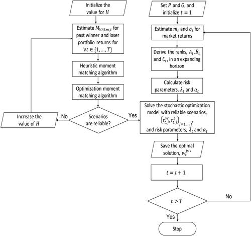
The procedure for scenario generation, reliability evaluation and stochastic portfolio optimization is outlined in Figure 3. To avoid data leakage, ideally we should use the early portion of the dataset as the training data set and the rest as the test data set, conduct scenario evaluation and parameter estimation using the training data, and apply the fixed parameter values to the test data. However, considering that the first momentum crash happened in 1932, there would not be sufficient training data to identify a suitable value of H while including this momentum crash in the test data set.

Figure 3. Flowchart for scenario generation, evaluation, and portfolio optimization.

5. Performance Evaluation

Suitable performance measures can provide straightforward quantitative criteria to evaluate the trading strategy derived by the stochastic program, the mean-variance model in Daniel and Moskowitz (2016), and the cross-sectional momentum heuristic ($w_t^W\equiv 1,w_t^L\equiv -1,$ and $w_t^f\equiv 1$), especially but not exclusively in market downturns.

Daniel and Moskowitz (2016) avoid momentum crashes using a variant of the Markowitz mean-variance model. They build an optimization model with the objective to maximize the Sharpe ratio of the portfolios, constructed by the winner minus loser portfolio and a risk-free asset, for the whole simulation horizon. This optimization model is equivalent to maximizing the long-term expected excess return of the winner minus loser portfolio subject to a constraint on return variance over the simulation horizon. They derive that the optimal weight on the past winner portfolio is $w_t^{W*}=\frac{{\mu }_t}{2\gamma {\delta }_t^2},$ where in period t, μ_t is the expectation of the difference between the past winner and past loser returns, in excess of the risk-free rate, and ${\delta }_t^2$ is the variance of the difference between the past winner and past loser returns. The parameter γ is chosen so that the in-sample annualized volatility, $\sqrt{\frac{N}{4{\gamma }^{2}T}{\sum }_{t=1}^{t=T}\frac{{\mu }_t^2}{{\delta }_t^2}},$ is 19%, which is the same as the annualized volatility of the CRSP value-weighted index over the full sample. Daniel and Moskowitz (2016) use a time series regression model to estimate μ_t and a GJR-GARCH model to forecast ${\delta }_t^2.$ As their strategy does not impose a limit on the proportion of wealth invested in the past winner and loser portfolios, the net short position of the past loser portfolios in their strategy would have reached a maximum of 5.37 in November 1952, which would incur a much higher transaction cost than the cross-sectional momentum heuristic and our mean-CVaR model. To allow a valid comparison between strategies, we compute μ_t as the difference between $M_{\mathit{VALmean},t}$ for past winners and $M_{\mathit{VALmean},t}$ for past losers, less $r_t^f,$ and ${\delta }_t^2$ as the variance of the difference between past winner and past loser returns in the past H periods; and we impose the constraint $-1\le w_t^{W*}\le 1.$

To evaluate these three types of strategies, multiple annualized performance measures, including the excess return, maximum drawdown, Sharpe ratio, upside potential ratio, and time series cumulative returns are considered.

A backtesting simulation is conducted to obtain these performance measures. Let $w_t^{W*}$ be the optimal weight for the winner portfolio in period t, and $r_t^W$ (resp. $r_t^L$) be the observed return for the winner (loser) portfolio in period t. Then we can derive the realized return for the constructed portfolio in period t, r_t, for $t=1,\dots ,T$: (23) $$r_t=w_t^{W*}(r_t^W-r_t^L)+r_t^f$$(23)

Annualized excess returns and annualized volatility are two basic measures of the overall gain and risk. They are calculated respectively as (24) $$EX=\frac{N}{T}\sum _{t=1}^T(r_t-r_t^f)$$(24) and (25) $$VO=\sqrt{\frac{N}{T-1}\sum _{t=1}^T{\left(r_t-\frac{\sum _{i=1}^T{r}_i}{T}\right)}^2}.$$(25)

However, volatility suffers from the weakness of treating upside potential and downside risk equally. This implies that using volatility as risk guidance may abandon a seemingly high-risk strategy that actually has high returns. Maximum drawdown (Young, 1991), the maximum observed loss from a peak to a trough of a portfolio before a new peak is attained, can overcome the drawback of volatility by only studying the downside risk and better detect the occurrence of momentum crashes. We calculate it using the maxDrawdown function in the PerformanceAnalytics R package (Peterson et al., 2014).

All the performance measures mentioned above focus on either risk or return but not both. They cannot tell investors whether the risk is worth the reward. The Sharpe ratio (Sharpe, 1966) is one of the most widely-used risk-adjusted metrics which takes account of both investment’s profit and the degree of risk that is taken to achieve it. Annualized Sharpe ratio can be calculated as (26) $$SR=\frac{EX}{VO}.$$(26)

Similar to the disadvantage of using volatility as the risk measure, Sharpe ratio is not able to differentiate between the upside reward and the downside risk. Compared to the Sharpe ratio, the upside potential ratio (UP ratio), proposed by Sortino and Van Der Meer (1991), is a more appropriate risk-adjusted performance measure, which measures the upside performance of portfolio returns for each unit of downside risk. The annualized UP ratio can be calculated as (27) $$UP=\frac{\frac{N}{T}\sum _{t=1}^T\max (0,r_t-r_t^f)}{\sqrt{\frac{N}{T}\sum _{t=1}^T{\left(\max (0,r_t^f-r_t)\right)}^2}}$$(27)

Finally, to investigate whether our proposed mean-CVaR optimization model with time-varying risk aversion can avoid momentum crashes and make profit in all market conditions, the time series cumulative absolute return is plotted. The cumulative absolute return up to time t is (28) $$C{A}_t={\Pi }_{i=1}^{i=t}(1+r_i).$$(28)

6. Numerical Results

Our data source is the Center for Research in Security Prices (www.crsp.com), where all monthly returns and prices of stocks listed on NYSE, AMEX, and NASDAQ with the returns of the common shares (with CRSP sharecode of 10 or 11) and VIX can be found. Following Daniel and Moskowitz (2016), the look-back period K = 12, and the holding period H = 1. The simulation horizon for the scenario generation process covers the end of each month from January 31, 1927, to December 31, 2020. VIX is available only from Feb 1, 1990. The number of generated scenarios, J, is set to be 10 for each instance. It is larger than the minimum J so that overspecifications can be avoided and differences in the value of α_t are meaningful, but small enough to avoid underspecification. The user-specified weights, v_m, for all statistics in the moment-matching scenario generation procedure are set to be 1/9. The values of pre-specified statistical properties, $M_{\mathit{VALm},t},$ are calculated using the preceding 3, 6, 9 and 12-month returns on a rolling basis; i.e., $H\in \{3,6,9,12\}.$ The number of months used to estimate the mean of index returns, P, and the number of months used to estimate the market volatility, G, are both selected from {3, 6, 9, 12}. All the statistical simulations and analyses are conducted using the R language.

Table 1 displays the value of the W² statistic and its p-value in the reliability test for three types of scenarios generated using different numbers of months to calculate each $M_{\mathit{VALm},t}.$ This table indicates that using past 12-month data to calculate $M_{\mathit{VALm},t}$ provides the smallest value of W² for the scenarios of the winner and loser returns, and thus, the best reliability for these two types of scenarios. By comparing the value of W² for winners and losers, we can see that the W² value of winners is smaller than that of losers for all tested values, which is consistent with the observation in Daniel and Moskowitz (2016) that the trend of loser portfolio returns is harder to predict and the momentum crashes are due mostly to such unforeseeable behavior of loser portfolios. Figure 4 displays the empirical density plots of returns for the winner and loser returns during the whole simulation horizon. The large excess kurtosis value of the loser returns also verifies that the loser has extreme returns occasionally, making its scenario generation less reliable. In terms of the reliability for the joint scenarios, using the past 9-month returns to calculate $M_{\mathit{VALm},t}$ shows the best performance and is the only one passing the reliability test. By examination of this table, we find that using H = 9 provides not only the best reliability for joint scenarios but also a decent performance for the scenarios of the winner and loser returns.

Figure 4. Empirical density plot of returns for the past winner and loser portfolios with mean, median, mode, skewness, and excess kurtosis shown during the whole simulation horizon.

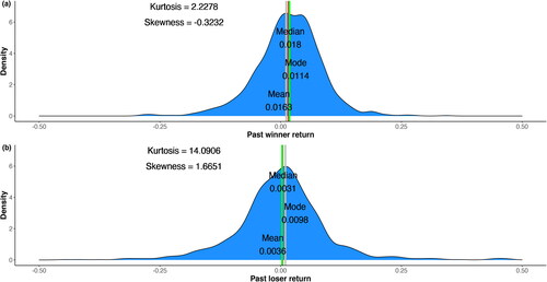
Table 1. W² statistic for the reliability of scenarios generated using various numbers of months, H, to calculate each $M_{\mathit{VALm},t}.$ The p-values computed by the dgof package are shown in parentheses.

H	3	6	9	12
Joint scenarios	5.5357 (0.0000)	2.5632 (0.0000)	0.2980 (0.1371)	1.3193 (0.0003)
Scenarios of past winner returns	4.3766 (0.0000)	1.2742 (0.0003)	0.1418 (0.4124)	0.0888 (0.6330)
Scenarios of past loser returns	7.6213 (0.0000)	2.2046 (0.0002)	0.6347 (0.0186)	0.1464 (0.3979)

Note that the simulation rather than the default approximation had to be used for at least one value in the table.

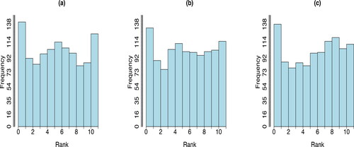
Figure 5 displays the generated scenarios for the joint winner and loser, winner marginal, and loser marginal returns when H = 9. All three subplots appear nearly flat, which further confirms that using past 9-month data to estimate $M_{\mathit{VALm},t}$ in this hybrid moment-matching algorithm produces scenarios that well represent the underlying uncertainty. Most importantly, the flatness of these plots promotes confidence that, upon employing these reliable scenarios in the stochastic portfolio optimization model on a rolling basis, asset allocation decisions derived from the solutions may avoid momentum crashes. Therefore, H = 9 is fixed for the following analysis.

Figure 5. MTD rank histogram for (a) joint past winner and loser scenarios, (b) scenarios of past winner returns, and (c) scenarios of past loser returns using past 9-month data to calculate $M_{\mathit{VALm},t}$ on a rolling basis and scenario sets of cardinality 10.

Table 2 presents a performance comparison among the baseline strategy (cross-sectional (CS) momentum heuristic), the mean-variance optimization model, and mean-CVaR optimization models with time-varying risk aversion defined by estimated market volatility in terms of annualized excess return, maximum drawdown, Sharpe ratio, and UP ratio. Different numbers of months to estimate the mean ($P\in \{3,6,9,12\}$) and to estimate the volatility of market index returns ($G\in \{3,6,9,12\}$) are considered for adjusting α_t and λ_t. This table indicates that the performance of the mean-CVaR models dominates the cross-sectional momentum heuristic and the mean-variance model. No matter which candidate value of P and G is selected, mean-CVaR always provides a higher excess return, Sharpe ratio, and UP ratio, as well as a smaller maximum drawdown, than the cross-sectional momentum heuristic or the mean-variance model. When p = 6 and G = 3, mean-CVaR offers the highest excess return, Sharpe ratio, and UP ratio, as well as the smallest maximum drawdown. Furthermore, the difference in the performance of all mean-CVaR models is trivial, which indicates that the mean-CVaR model with volatility-adjusted risk aversion is robust to the values of P and G.

Table 2. Annualized performance comparison among the baseline strategy (CS momentum heuristic), the mean-variance optimization model, and the mean-CVaR optimization models with time-varying risk aversions defined by estimated market volatility when H = 9.

Strategy	Excess return	Maximum drawdown	Sharpe ratio	UP ratio
p = 6, G = 3	0.1669	0.5118	0.7757	2.5176
p = 12, G = 3	0.1657	0.5118	0.7684	2.5026
p = 9, G = 3	0.1650	0.5118	0.7637	2.4886
p = 3, G = 3	0.1635	0.5118	0.7585	2.4847
p = 3, G = 9	0.1643	0.5118	0.7754	2.4610
p = 6, G = 12	0.1642	0.5118	0.7805	2.4505
p = 9, G = 9	0.1606	0.5118	0.7626	2.4488
p = 6, G = 9	0.1610	0.5118	0.7649	2.4486
p = 9, G = 12	0.1606	0.5248	0.7586	2.4278
p = 12, G = 9	0.1568	0.5118	0.7454	2.4213
p = 12, G = 12	0.1592	0.5248	0.7520	2.4195
p = 6, G = 6	0.1615	0.6325	0.7596	2.4142
p = 3, G = 6	0.1591	0.6325	0.7522	2.3959
p = 9, G = 6	0.1570	0.6325	0.7387	2.3898
p = 3, G = 12	0.1601	0.5118	0.7492	2.3872
p = 12, G = 6	0.1554	0.6325	0.7332	2.3806
Mean-variance	0.1109	0.5118	0.6349	2.1496
CS momentum heuristic	0.1512	0.9674	0.5076	1.8855

This table is sorted by the descending up ratio.

For the performance of mean-CVaR with time-varying risk aversion parameters defined using the reward-risk ratio or VIX, we find that neither of them can provide a stronger performance than setting these parameter values using volatility. When using the reward-risk ratio to automate risk aversions, the mean-CVaR models underperform the mean-variance model and the cross-sectional momentum heuristic for all tested numbers of months used to estimate the market return and volatility. The mean-CVaR models using the VIX to define risk aversions produce a better maximum drawdown, Sharpe ratio, and UP ratio than the mean-variance model and the cross-sectional momentum heuristic but a lower excess return than the cross-sectional momentum heuristic. The details of the performance comparison are included in the online supplement.

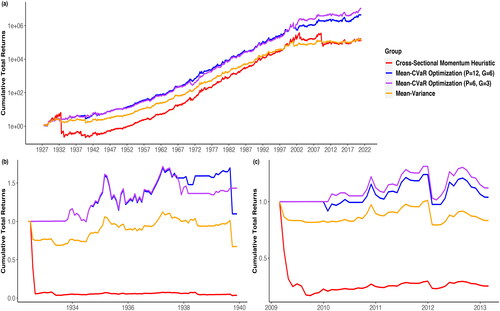
To check whether our mean-CVaR model with time-dependent risk aversion defined using estimated market volatility is profitable in various market conditions and avoids two momentum crashes, Figure 6 plots the time-series cumulative returns of the worst-performing ($P=6,G=3$) and the best-performing ($P=12,G=6$) mean-CVaR models during the whole simulation horizon in subplot (a), the first momentum crash in (b), and the second momentum crash in (c). Both mean-CVaR models consistently produce higher cumulative returns than either the cross-sectional momentum heuristic or the mean-variance model. One notable exception occurs during the Great Depression period (August 1929—March 1933), but the slopes of mean-CVaR returns are still positive, implying mean-CVaR still would have made a profit during the Great Depression. What is more, in both mean-CVaR models, there is no drastic decline during 1926-2020. The underperformance of the cross-sectional momentum heuristic is mostly due to the two momentum crashes. In the online supplement, we show that the cross-sectional momentum heuristic yields the best performance among these four strategies in terms of the cumulative total returns from January 1940 to December 2002, when the momentum crash periods are excluded. Note that Daniel and Moskowitz report much higher returns for the mean-variance strategy but they do not enforce the weight constraint for winner and loser portfolios. Very interestingly, we notice that despite the steep decline in the stock market due to COVID-19 in early 2020, there is no momentum crash for any strategy tested during the recovery period from April 2020 to December 2020, although the S&P 500 index increased by over 45%. This observation might be explained by the relatively modest stock market decline during the whole pandemic compared to the Great Depression or the Global Financial Crisis. For the two momentum crash periods, different from the dramatic sustained drawdown in the cross-sectional momentum heuristic, the cumulative returns of both mean-CVaR models are almost continuously above one, which means no great loss will be incurred during these two periods. Hence, our mean-CVaR model with time-dependent risk aversion successfully avoids momentum crashes. Note that the flat segments of the cumulative reward curves for the mean-CVaR optimization occur when it places zero weight on the winner-minus-loser portfolio. No optimal weights of −1 are observed in this backtest.

Figure 6. Time series cumulative returns of the cross-sectional momentum strategy, the mean-variance optimization model, and the mean-CVaR optimization model with time-varying risk aversions defined using the estimated market volatility during (a) the whole simulation horizon, (b) june 1932 - December 1939, the first momentum crash, following the Great Depression, and (c) March 2009 - March 2013, the second momentum crash, following the 2008-2009 financial crisis, when H = 9.

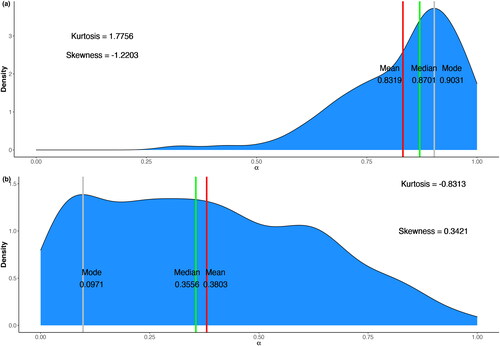
To further investigate the relationship between the risk parameters, α (= λ), defined using estimated market volatility and the optimal weight on the winner-minus-loser, $w^{*},$ we plot the conditional density distribution of α given (a) $w^{*}=0$ and (b) $w^{*}=1$ when p = 6 and G = 3. As shown in Figure 7, when α is 1, $w^{*}$ could be 1 or 0. This observation is consistent with Equation (13)(13) $$w^{W*}=\{\begin{array}{cc}-1,\hfill & \text{ if }(1-\lambda )\mathrm{E}[R^W-R^L]<-\lambda \text{CVaR}[R^W-R^L]\hfill \\ 0,\hfill & \text{ if }-\lambda \text{CVaR}[R^W-R^L]\le (1-\lambda )\mathrm{E}[R^W-R^L]\le \lambda \text{CVaR}[-(R^W-R^L)]\hfill \\ 1,\hfill & \text{ if }(1-\lambda )\mathrm{E}[R^W-R^L]>\lambda \text{CVaR}[-(R^W-R^L)]\hfill \end{array}$$(13) that the optimal weight on the winner-minus-losers relies on the combination of 1) generated scenarios, 2) α, and 3) λ. Although the optimal weight on the winner-minus-loser cannot be simply determined by the value of α or λ, Figure 7 shows it is more likely to have $w^{*}$ of 0 when α is close to 1 and have $w^{*}$ of 1 when α is close to 0, suggesting that it is more likely for the mean-CVaR model to recommend not longing the winner-minus-loser portfolio during an extreme volatile period to mitigate investment loss.

Figure 7. Empirical conditional density plot of α(λ) given (a) $w^{*}=0$ and (b) $w^{*}=1$ with mean, median, mode, skewness, and excess kurtosis shown during the whole simulation horizon.

7. Conclusion

The cross-sectional momentum strategy exhibits strong and consistent performance across many diverse asset classes and periods. However, the severe and unpredictable momentum crashes make this strategy unfavorable by many investors. In this paper, we develop a stochastic mean-CVaR optimization model with time-varying risk aversion, which successfully avoids momentum crashes. Furthermore, the simple structure of the optimal trading solution to our mean-CVaR model is an added value for its usage in the industry due to its efficient computation.

In this strategy, we deal with the uncertainty of the stock market that causes momentum crashes by a combination of three solutions. First, as momentum crashes are infrequent but costly, and thus can be regarded as extreme events, we utilize a downside risk measure, CVaR, to control the expected loss under the extreme case. Second, momentum crashes happen in panic states when the stock market is volatile. Therefore, we adopt time-dependent risk aversion, calculated based on estimated market volatility, which outperforms the estimated reward-risk ratio or volatility index, to flexibly and automatically adjust the investment strategy according to the changing market condition. Third, the return of momentum portfolios (past losers and past winners) is uncertain when making investment decisions. However, the existence of momentum crashes is a signal that the distribution of momentum portfolio returns has large kurtosis and the remarkable performance of the cross-sectional momentum strategy indicates momentum portfolios are highly correlated. To capture the inherent structure of the momentum portfolio returns, we apply a hybrid of heuristic and optimization moment-matching algorithms and generate scenarios that well represent the underlying uncertainty. The reliability of the generated scenarios is evaluated based upon Cramér-von Mises hypothesis testing for the uniformity of the MTD rank histogram.

By carrying out computational studies over a 95-year interval on common shares of all stocks listed on NYSE, AMEX, and NASDAQ, we find that reliable scenarios for the joint returns of the winners and losers, the winners only, and the losers only are generated when using nine months’ worth of past data to estimate the parameters in this scenario generation approach. Upon employing these reliable scenarios in the mean-CVaR model with time-dependent risk aversion parameters defined using estimated market volatility, the rebalanced portfolio shows performance that is robust to the number of periods for estimating market volatility and achieves higher excess returns, Sharpe ratio, and upside potential ratio, as well as lower maximum drawdown, than either the cross-sectional momentum heuristic or the mean-variance model. We observe no drastic decline in the time series cumulative returns throughout the whole simulation horizon. Particularly during the two momentum crash periods, the cumulative returns of mean-CVaR are maintained around the level of one, indicating no huge loss is incurred when using this mean-CVaR model and the momentum crashes are avoided. Through further investigation of the empirical conditional density distribution of the risk parameters given the optimal weight on the momentum portfolio, we conclude that, while the optimal weight on the winner-minus-loser cannot be simply determined by the value of risk parameters, it is more likely for our mean-CVaR strategy to suggest not longing the winner-minus-loser when the stock market is extremely volatile.

For future research, we plan to explore various approaches to automate risk aversion. For example, empirical research shows that clients’ risk aversion changes in response to shocks to client demographics (Barsky et al., 1997; Guiso & Paiella, 2008) and market returns and economic conditions (Bucciol & Miniaci, 2018; Guiso et al., 2018). Therefore, in addition to market volatility, reward-risk ratio, and VIX, we can consider other signals to automate the change in risk aversion settings. Moreover, robo-advisors, which collect information from clients about their financial situation, risk attitudes, and future goals through an online survey and then use the data to offer advice and automatically invest client assets, have emerged as an alternative to traditional financial advisors due to their high portfolio personalization, affordable portfolio management, and full automation for portfolio construction and rebalancing (D’Acunto et al., 2019; D’Acunto & Rossi, 2020; Jung et al., 2018). The current approach to incorporate risk aversion in robo-advisors involves human-machine interaction. Extending robo-advising algorithms to automatically adjust risk aversion appears promising. Last but not least, a more general momentum heuristic accounting for volatility that could outperform our mean-CVaR model would be another interesting topic to investigate.

Additional information

Notes on contributors

Xiaoshi Guo

Xiaoshi Guo received a doctoral degree in Industrial Engineering from Iowa State University, USA, in 2021, a master’s degree in Industrial Engineering from the University of Pittsburgh, USA, in 2017, and a bachelor’s degree in Mathematics from Sichuan University, China, in 2015. Her research interests include stochastic programming, risk analysis, and their applications in financial portfolio optimization. She is a member of Institute for Operations Research and the Management Sciences and Institute of Industrial and Systems Engineers.

Sarah M. Ryan

Sarah M. Ryan is the C. G.“Turk” and Joyce A. Therkildsen Department Chair and Professor of Industrial and Manufacturing Systems Engineering at Iowa State University. With expertise in stochastic modeling and optimization under uncertainty, Dr. Ryan directs the DataFEWSion National Research Traineeship for Innovations at the Nexus of Food Production, Renewable Energy, and Water Quality Systems. She previously served as the Editor-in-Chief of The Engineering Economist. Her research has been supported by the National Science Foundation, including a CAREER Award, the US Department of Energy, the Iowa Energy Center, an AT&T Industrial Ecology Faculty Fellowship, and industry consortia. She is a Fellow of the Institute of Industrial and Systems Engineers.

References

- Ahmadi-Javid, A. (2012). Entropic value-at-risk: A new coherent risk measure. Journal of Optimization Theory and Applications, 155(3), 1105–1123. https://doi.org/10.1007/s10957-011-9968-2
- Ahmadi-Javid, A., & Fallah-Tafti, M. (2019). Portfolio optimization with entropic value-at-risk. European Journal of Operational Research, 279(1), 225–241. https://doi.org/10.1016/j.ejor.2019.02.007
- Arnold, T. B., & Emerson, J. W. (2011). Nonparametric goodness-of-fit tests for discrete null distributions. R Journal, 3(2), 34–39.
- Asness, C. S., Frazzini, A., & Pedersen, L. H. (2012). Leverage aversion and risk parity. Financial Analysts Journal, 68(1), 47–59. https://doi.org/10.2469/faj.v68.n1.1
- Asness, C. S., Liew, J. M., & Stevens, R. L. (1997). Parallels between the cross-sectional predictability of stock and country returns. The Journal of Portfolio Management, 23(3), 79–87. https://doi.org/10.3905/jpm.1997.409606
- Bae, G. I., Kim, W. C., & Mulvey, J. M. (2014). Dynamic asset allocation for varied financial markets under regime switching framework. European Journal of Operational Research, 234(2), 450–458. https://doi.org/10.1016/j.ejor.2013.03.032
- Banihashemi, S., & Navidi, S. (2017). Portfolio performance evaluation in mean-CVaR framework: A comparison with non-parametric methods value at risk in Mean-VaR analysis. Operations Research Perspectives, 4, 21–28. https://doi.org/10.1016/j.orp.2017.02.001
- Barro, D., Canestrelli, E., & Consigli, G. (2019). Volatility versus downside risk: Performance protection in dynamic portfolio strategies. Computational Management Science, 16(3), 433–479. https://doi.org/10.1007/s10287-018-0310-4
- Barroso, P., & Santa-Clara, P. (2015). Momentum has its moments. Journal of Financial Economics, 116(1), 111–120. https://doi.org/10.1016/j.jfineco.2014.11.010
- Barsky, R. B., Juster, F. T., Kimball, M. S., & Shapiro, M. D. (1997). Preference parameters and behavioral heterogeneity: An experimental approach in the health and retirement study. The Quarterly Journal of Economics, 112(2), 537–579. https://doi.org/10.1162/003355397555280
- Benati, S., & Conde, E. (2022). A relative robust approach on expected returns with bounded CVaR for portfolio selection. European Journal of Operational Research, 296(1), 332–352. https://doi.org/10.1016/j.ejor.2021.04.038
- Bergk, K., Brandtner, M., & Kürsten, W. (2021). Portfolio selection with tail nonlinearly transformed risk measures—A comparison with mean-CVaR analysis. Quantitative Finance, 21(6), 1011–1025. https://doi.org/10.1080/14697688.2020.1856912
- Bucciol, A., & Miniaci, R. (2018). Financial risk propensity, business cycles and perceived risk exposure. Oxford Bulletin of Economics and Statistics, 80(1), 160–183. https://doi.org/10.1111/obes.12193
- Chen, A. H., Fabozzi, F. J., & Huang, D. (2012). Portfolio revision under mean-variance and mean-CVaR with transaction costs. Review of Quantitative Finance and Accounting, 39(4), 509–526. https://doi.org/10.1007/s11156-012-0292-1
- Choulakian, V., Lockhart, R. A., & Stephens, M. A. (1994). Cramér-von Mises statistics for discrete distributions. Canadian Journal of Statistics, 22(1), 125–137. https://doi.org/10.2307/3315828
- Cui, T., Bai, R., Ding, S., Parkes, A. J., Qu, R., He, F., & Li, J. (2020). A hybrid combinatorial approach to a two-stage stochastic portfolio optimization model with uncertain asset prices. Soft Computing, 24(4), 2809–2831. https://doi.org/10.1007/s00500-019-04517-y
- D’Acunto, F., Prabhala, N., & Rossi, A. G. (2019). The promises and pitfalls of robo-advising. The Review of Financial Studies, 32(5), 1983–2020. https://doi.org/10.1093/rfs/hhz014
- D’Acunto, F., & Rossi, A. G. (2020). Robo-advising. Available at SSRN 3545554.
- Daniel, K., & Moskowitz, T. J. (2016). Momentum crashes. Journal of Financial Economics, 122(2), 221–247. https://doi.org/10.1016/j.jfineco.2015.12.002
- Grinblatt, M., & Titman, S. (1993). Performance measurement without benchmarks: An examination of mutual fund returns. The Journal of Business, 66(1), 47–68. https://doi.org/10.1086/296593
- Grobys, K., Ruotsalainen, J., & Äijö, J. (2018). Risk-managed industry momentum and momentum crashes. Quantitative Finance, 18(10), 1715–1733. https://doi.org/10.1080/14697688.2017.1420211
- Guiso, L., & Paiella, M. (2008). Risk aversion, wealth, and background risk. Journal of the European Economic Association, 6(6), 1109–1150. https://doi.org/10.1162/JEEA.2008.6.6.1109
- Guiso, L., Sapienza, P., & Zingales, L. (2018). Time varying risk aversion. Journal of Financial Economics, 128(3), 403–421. https://doi.org/10.1016/j.jfineco.2018.02.007
- Guo, X., Chan, R. H., Wong, W.-K., & Zhu, L. (2019). Mean–variance, mean–VaR, and mean–CVaR models for portfolio selection with background risk. Risk Management, 21(2), 73–98. https://doi.org/10.1057/s41283-018-0043-2
- Guo, X., & Ryan, S. M. (2021). Reliability assessment of scenarios generated for stock index returns incorporating momentum. International Journal of Finance & Economics, 26(3), 4013–4031. https://doi.org/10.1002/ijfe.2002
- Guo, X., & Ryan, S. M. (2021a). Portfolio rebalancing based on time series momentum and downside risk. IMA Journal of Management Mathematics, 34(2), 355–381. https://doi.org/10.1093/imaman/dpab037
- Guo, X., & Ryan, S. M. (2021b). Scenario generation for asset returns in a cross-sectional momentum strategy. In Proceedings of the 2021 IISE Annual Conference.
- Høyland, K., Kaut, M., & Wallace, S. W. (2003). A heuristic for moment-matching scenario generation. Computational Optimization and Applications, 24(2/3), 169–185. https://doi.org/10.1023/A:1021853807313
- Høyland, K., & Wallace, S. W. (2001). Generating scenario trees for multistage decision problems. Management Science, 47(2), 295–307. https://doi.org/10.1287/mnsc.47.2.295.9834
- Hsu, W-r., & Murphy, A. H. (1986). The attributes diagram a geometrical framework for assessing the quality of probability forecasts. International Journal of Forecasting, 2(3), 285–293. https://doi.org/10.1016/0169-2070(86)90048-8
- Jegadeesh, N., & Titman, S. (1993). Returns to buying winners and selling losers: Implications for stock market efficiency. The Journal of Finance, 48(1), 65–91. https://doi.org/10.1111/j.1540-6261.1993.tb04702.x
- Jung, D., Dorner, V., Weinhardt, C., & Pusmaz, H. (2018). Designing a robo-advisor for risk-averse, low-budget consumers. Electronic Markets, 28(3), 367–380. https://doi.org/10.1007/s12525-017-0279-9
- Kim, K., & Park, C. S. (2021). Pricing real options based on linear loss functions and conditional value at risk. The Engineering Economist, 66(1), 3–26. https://doi.org/10.1080/0013791X.2020.1867273
- Kim, Y. S., Giacometti, R., Rachev, S. T., Fabozzi, F. J., & Mignacca, D. (2012). Measuring financial risk and portfolio optimization with a non-Gaussian multivariate model. Annals of Operations Research, 201(1), 325–343. https://doi.org/10.1007/s10479-012-1229-8
- Ledoit, O., & Wolf, M. (2003). Improved estimation of the covariance matrix of stock returns with an application to portfolio selection. Journal of Empirical Finance, 10(5), 603–621. https://doi.org/10.1016/S0927-5398(03)00007-0
- Ledoit, O., & Wolf, M. (2004 a). Honey, I shrunk the sample covariance matrix. The Journal of Portfolio Management, 30(4), 110–119. https://doi.org/10.3905/jpm.2004.110
- Ledoit, O., & Wolf, M. (2004 b). A well-conditioned estimator for large-dimensional covariance matrices. Journal of Multivariate Analysis, 88(2), 365–411. https://doi.org/10.1016/S0047-259X(03)00096-4
- Lehmann, B. N. (1990). Fads, martingales, and market efficiency. The Quarterly Journal of Economics, 105(1), 1–28. https://doi.org/10.2307/2937816
- Li, H., Wu, C., & Zhou, C. (2022). Time-varying risk aversion and dynamic portfolio allocation. Operations Research, 70(1), 23–37. https://doi.org/10.1287/opre.2020.2095
- Lim, A. E., Shanthikumar, J. G., & Vahn, G.-Y. (2011). Conditional value-at-risk in portfolio optimization: Coherent but fragile. Operations Research Letters, 39(3), 163–171. https://doi.org/10.1016/j.orl.2011.03.004
- Markowitz, H. (1952). Portfolio selection. Journal of Finance, 7(1), 77–91. https://doi.org/10.2307/2975974
- Moazeni, S., Coleman, T. F., & Li, Y. (2016). Smoothing and parametric rules for stochastic mean-CVaR optimal execution strategy. Annals of Operations Research, 237(1-2), 99–120. https://doi.org/10.1007/s10479-013-1391-7
- Okunev, J., & White, D. (2003). Do momentum-based strategies still work in foreign currency markets? Journal of Financial and Quantitative Analysis, 38(2), 425–447. https://doi.org/10.2307/4126758
- Peterson, B. G., Carl, P., Boudt, K., Bennett, R., Ulrich, J., & Zivot, E. (2014). PerformanceAnalytics: Econometric tools for performance and risk analysis. R Package Version, 1(3541), 107.
- Pflug, G. C. (2000). Some remarks on the value-at-risk and the conditional value-at-risk. In S. Uryasev (Ed.), Probabilistic constrained optimization: methodology and applications (pp. 272–281). Springer.
- Pflug, G. C., & Pichler, A. (2016). Time-inconsistent multistage stochastic programs: Martingale bounds. European Journal of Operational Research, 249(1), 155–163. https://doi.org/10.1016/j.ejor.2015.02.033
- Ripley, B. D. (1987). Stochastic simulation. John Wiley & Sons.
- Rockafellar, R. T., & Uryasev, S. (2000). Optimization of conditional value-at-risk. The Journal of Risk, 2(3), 21–41. https://doi.org/10.21314/JOR.2000.038
- Rockafellar, R. T., & Uryasev, S. (2002). Conditional value-at-risk for general loss distributions. Journal of Banking & Finance, 26(7), 1443–1471. https://doi.org/10.1016/S0378-4266(02)00271-6
- Sar I, D., Lee, Y., Ryan, S., & Woodruff, D. (2016). Statistical metrics for assessing the quality of wind power scenarios for stochastic unit commitment. Wind Energy, 19(5), 873–893. https://doi.org/10.1002/we.1872
- Sharifi, M., & Kwon, R. H. (2018). Performance-based contract design under cost uncertainty: A scenario-based bilevel programming approach. The Engineering Economist, 63(4), 291–318. https://doi.org/10.1080/0013791X.2018.1467990
- Sharifi, M., Kwon, R. H., & Jardine, A. K. (2016). Valuation of performance-based contracts for capital equipment: A stochastic programming approach. The Engineering Economist, 61(1), 1–22. https://doi.org/10.1080/0013791X.2015.1081711
- Sharpe, W. F. (1966). Mutual fund performance. The Journal of Business, 39(S1), 119–138. https://doi.org/10.1086/294846
- Sortino, F. A., & Van Der Meer, R. (1991). Downside risk. The Journal of Portfolio Management, 17(4), 27–31. https://doi.org/10.3905/jpm.1991.409343
- Thomann, A. (2021). Multi-asset scenario building for trend-following trading strategies. Annals of Operations Research, 299(1–2), 293–315. https://doi.org/10.1007/s10479-020-03547-2
- Topaloglou, N., Vladimirou, H., & Zenios, S. A. (2011). Optimizing international portfolios with options and forwards. Journal of Banking & Finance, 35(12), 3188–3201. https://doi.org/10.1016/j.jbankfin.2011.05.003
- Whaley, R. E. (2009). Understanding the VIX. The Journal of Portfolio Management, 35(3), 98–105. https://doi.org/10.3905/JPM.2009.35.3.098
- Xiong, J. X., & Idzorek, T. M. (2011). The impact of skewness and fat tails on the asset allocation decision. Financial Analysts Journal, 67(2), 23–35. https://doi.org/10.2469/faj.v67.n2.5
- Young, T. W. (1991). Calmar ratio: A smoother tool. Futures, 20(1), 40.
- Yu, L.-Y., Ji, X.-D., & Wang, S.-Y. (2003). Stochastic programming models in financial optimization: A survey. AMO - Advanced Modeling and Optimization, 5(1), 1–26.
- Zou, J., Ahmed, S., & Sun, X. A. (2019). Stochastic dual dynamic integer programming. Mathematical Programming, 175(1–2), 461–502. https://doi.org/10.1007/s10107-018-1249-5