The Tax Benefits of Separating Alpha from Beta

Abstract

Long-only active investment strategies have an inherent flaw: Investors pay capital gains taxes on market-related gains as well as on the alpha created. By separating alpha and beta, taxes can be reduced and returns enhanced. 

Using both simulated and historical data, we show that separating active returns (i.e., alpha) from market exposure (i.e., beta) may have significant tax benefits. We find that an investment strategy that invests separately in a passive index portfolio and an actively managed long–short portfolio is more tax efficient than a long-only actively managed strategy with similar risk and style exposures. The turnover of a traditional active strategy causes capital gain realizations in both the active and passive portfolio components. In contrast, the turnover of a strategy that separates alpha from beta is concentrated in the long–short component and enables the deferral of capital gain realizations in the passive market component. Separating alpha from beta is different from systematic tax management as described in the literature. Our approach provides a practical solution for taxable investors in a world dominated by tax-agnostic managers.

Disclosure: AQR Capital Management is a global investment management firm that may or may not apply investment techniques or methods of analysis similar to those described herein. The views expressed here are those of the authors and not necessarily those of AQR. The reader should conduct his or her own analysis and consult with professional advisers prior to making any investment decisions. AQR is not a tax adviser. This material is intended for informational purposes only and should not be construed as legal or tax advice, nor is it intended to replace the advice of a qualified attorney or tax adviser.

Editor’s Notes

Submitted 22 March 2019

Accepted 11 September 2019 by Stephen J. Brown

This article was externally reviewed using our double-blind peer-review process. When the article was accepted for publication, the authors thanked the reviewers in their acknowledgments. Benjamin Schneider, CFA, was one of the reviewers for this article.

Traditional long-only active strategies often require high turnover to implement the views of the portfolio manager, which triggers the realization of capital gains from both the active and the passive exposures. In contrast, an investment portfolio that separates active and passive exposures enables deferral of the realization of capital gains in the passive component.¹ Thus, the separation of alpha from beta is relevant for taxable investors—such as individuals and family offices, in particular, because they do not face regulatory constraints on their ability to implement strategies requiring leverage and short selling.

The alpha–beta separation approach to enhancing the tax efficiency of actively managed strategies in a taxable account is distinct from two other approaches proposed in the literature—namely, systematic tax management² and relaxed-constraint portfolio construction.³ Although a number of active tax-managed and relaxed-constraint funds exist and some asset management platforms offer active tax-managed strategies through separate accounts, the universe of investment offerings is dominated by traditional long-only funds and accounts, long–short funds, and passive indexed mutual funds and exchange-traded funds (ETFs). As a result, our alpha–beta separation approach can improve the tax efficiency of an investment portfolio in many realistic scenarios where desired strategies are offered only through typical tax-agnostic long-only and long–short vehicles.⁴

In this article, we illustrate the tax benefits of our approach to investment portfolio design by comparing two quantitative investment strategies. The first strategy is a traditional “long-only” (LO) strategy that overweights stocks with favorable factor exposures and underweights stocks with unfavorable factor exposures in order to outperform the market. The strategy turns over portfolio positions as stocks’ relative attractiveness changes over time. The second strategy is a “composite long–short” (CLS) strategy that allocates separately to a passively managed index portfolio and an actively managed long–short portfolio. The index portfolio component constitutes a beta-one exposure to the equity market and requires minimal turnover (for example, it might be a broadly diversified index mutual fund or ETF). The active component of the allocation corresponds to a market-neutral long–short portfolio that is constructed to achieve desired style factor exposures with no exposure to the aggregate equity market. Like the long-only portfolio, the long–short component of the composite strategy requires turnover to reflect changes in the relative attractiveness of stocks. The LO and CLS strategies are designed in such a way that they target similar exposures to the market and other factors. Although our analysis focuses on quantitative factor-based strategies, our results can be generalized to other active strategies.

A comparison of such investment approaches was originally performed by Means (2002). Means used a numerical example with deterministic returns, turnover, and levels of realization of long-term and short-term capital gains. In the study reported here, we confirmed Means’s conclusions pertaining to the tax benefits of separating alpha from beta and expanded his analysis as follows. First, we used trading patterns of well-known quantitative factor strategies to model tax outcomes. Second, we used a Monte Carlo simulation environment where we could control and vary return distribution parameters and compare the tax efficiency of factor strategies constructed within this environment. Finally, we constructed factor strategies from historical data to test whether the conclusions of the Monte Carlo simulations held when real data were used.⁵

The Monte Carlo simulation methodology allowed us to generate numerous return histories for diversified portfolios implementing a value/momentum strategy. We found that for a similar level of pretax returns, the composite long–short strategy reliably outperformed the long-only strategy after taxes. For example, the long-only strategy based on value and momentum generated an average after-tax return of 8.1% and an after-tax alpha of 0.6% per year. In contrast, a composite long–short strategy generated an average after-tax return of 9.4% and an after-tax alpha of 1.9% per year. Separating alpha from beta resulted in higher after-tax returns in each of our 100 simulated return histories. Moreover, the tax benefits of separating the active and passive components of a portfolio increased with the expected market return and the strategy portfolio turnover. We document that our results are robust to alternative assumptions about return distribution, different tax rates, transaction and financing costs, expenses and management fees, and liquidation taxes.

Historical strategy simulations with real US market data for the period 1985 to 2018 confirmed these Monte Carlo results. The after-tax alphas gross of costs and fees were 1.7% for the CLS strategy and –0.2% for the LO strategy. Consistent with the Monte Carlo simulations, we found that the tax savings of the composite strategy increased with the level of market return and portfolio turnover. The fact that we observed similar outcomes in the Monte Carlo environment and historical data indicates that our results are neither driven by Monte Carlo parameterization nor confined to a specific market history.

The superior performance of the composite strategy occurs because the necessary turnover of a long-only strategy generates taxes on both the passive market return and the active excess return whereas the turnover of the combined strategy is focused solely on the long–short active component. The composite strategy thus realizes taxable capital gains only on the actively managed long–short component; the passive component enables the deferral of capital gains. The deferral of capital gains is beneficial for several reasons. First, taxes on long-term capital gains are lower than taxes on short-term capital gains. Second, the present value of the tax burden decreases if the payment of capital gains taxes is deferred to future years. Third, capital gains taxes can be completely avoided if the appreciated assets pass through an estate (because of the step-up of the cost basis at death) or if the assets are donated to a charity.

A composite strategy also has significant tax advantages when an investor decides to switch active managers. The replacement of a manager leads to capital gain realizations if the manager’s portfolio has a capital gains overhang. Because of the reluctance of investors to realize capital gains, they might be “locked in” with respect to their manager allocations, as discussed by, among many others, Holt and Shelton (1962), Stein and Narasimhan (1999), and Lucas and Sanz (2016). This lock-in effect is mitigated for composite long–short strategies because the investor needs to replace only the active component of the strategy. The passive component, which might have experienced a significant appreciation over time, remains untouched. Furthermore, manager changes typically occur as a result of disappointing performance. Thus, liquidating the active portion of the strategy might not cause large capital gains realizations and might even lead to the benefit of realizing capital losses.

This article contributes to the literature on the taxation of active investment strategies. Jeffrey and Arnott (1993); Dickson and Shoven (1995); Bergstresser and Poterba (2002); Bergstresser and Pontiff (2013); Arnott, Kalesnik, and Schuesler (2018); and Sialm and Zhang (forthcoming) documented that the tax costs of active long-only investment strategies often more than offset the pretax manager alpha. Goldberg, Hand, and Cai (2019) examined the tax efficiency of various factor-based strategies and showed that systematic tax management may add significant value for taxable investors. Israel, Moskowitz, Ross, and Serban (2017) compared several tax-managed long-only momentum mutual funds with funds implementing identical strategies but without tax management and found that, on average, tax management improved after-tax returns by 80 basis points (bps) per year. Sialm and Sosner (2018) and Sosner, Krasner, and Pyne (2019) showed that the after-tax performance of factor-based tax-managed strategies can be enhanced by relaxing the long-only constraint. Whereas the tax benefits of systematic tax management and shorting are well documented in the literature, the benefit of separating alpha from beta is rarely mentioned, even though it might be the most practical approach to tax efficiency in a world dominated by tax-agnostic active strategies. Moreover, as we also show in this article, alpha–beta separation can be combined with tax management of the alpha strategy to further enhance tax efficiency.

Performance of Strategies in Monte Carlo Simulations

In this section, we compare the Monte Carlo simulation results of a long-only strategy with the results of a composite strategy that allocates to a passive investment in the market portfolio and an actively managed market-neutral long–short strategy. In the base case, transaction and financing costs and fees are not included.

Methodology and Assumptions.

We explain here the main aspects of the methodology and the assumptions used in our Monte Carlo simulations. The detailed methodology is provided in Appendix A.

We simulated returns from a multifactor distribution for 500 stocks. The simulated portfolios were updated monthly for a period of 25 years. Furthermore, each return history was simulated 100 times to obtain a distribution of return histories. Most of our results correspond to the average results over the 100 simulations. Where relevant, however, we report the distribution of results across simulations. We assumed that all the returns are price returns and did not model dividend payments. Hence, our simulated strategy generated only capital gains, no dividend income. This simplifying assumption was reasonable for our purpose of measuring differences between long-only and composite long–short strategies because their dividends are likely to be similar.

Our model incorporated market, value, and momentum factors. The value factor was proxied by a long-term reversal and depended negatively on the performance over the prior 60 months. The momentum factor depended positively on the performance over the prior 12 months excluding the most recent month. This specification was motivated by the fact that value and momentum styles have persisted among various asset classes, markets, and time periods, as documented by Asness, Moskowitz, and Pedersen (2013). From a tax perspective, value signals are negatively related to past returns, whereas momentum signals are positively related to past returns, which generates interesting tax dynamics, as documented by Israel and Moskowitz (2012).

In the base case, we assumed for the market factor an annualized mean return of 8% and a volatility of 15%. For the value and momentum style factors, we assumed an annual average return of 2% and a volatility of 4% each.⁶ The market factor was assumed to be uncorrelated with the value and momentum factors, whereas the correlation between the value and momentum factors was set at −0.7.⁷ All stocks were assumed to have a constant beta of 1.0 to the market factor. Stocks’ exposures to the value and momentum factors varied dynamically on the basis of the stocks’ simulated price histories. The annualized stock-specific volatility was set equal to 25% for each stock.

In the Monte Carlo simulations, we used a simple heuristic method for portfolio construction. We ranked stocks on the basis of their value and momentum exposures, summed up the value and momentum ranks, and ranked again to obtain a combined value/momentum rank. The ranks were then demeaned so that half of the stocks had a positive factor score and half of the stocks had a negative factor score. For the long-only strategy, the negative ranks were dismissed and the positive ranks were rescaled to sum to 100%. For the long–short component of the composite strategy, positive and negative scores were each rescaled to sum to 50%, resulting in a total gross notional exposure of 100%. The investor used each $1 of capital invested in the passive index fund—for example, an ETF or open-end mutual fund—to margin $1 of gross notional exposure of the long–short strategy, $0.50 long and $0.50 short. For practical purposes, the long–short portion of the composite strategy can be thought of as investment in a market-neutral hedge fund or a market-neutral mutual fund.

We calibrated the two-sided turnover as a percentage of portfolio net asset value (NAV) of the value/momentum strategies at 180% per year. Two-sided turnover takes into account both acquisitions and dispositions of stocks. An annual two-sided turnover of 180% is consistent with the turnover of actively managed US open-end mutual funds, as reported by Edelen, Evans, and Kadlec (2013). The simulation environment allowed us to control the return characteristics in such a way that returns and risk exposures of long–short and long-only portfolios closely matched each other. Thus, we could focus on the tax implications of the two approaches while holding the pretax returns approximately constant.

Tax Computation.

We assumed that long-term gains were taxed at a 20% rate and short-term gains were taxed at a 35% rate.⁸ We kept track of the individual tax lots of the portfolio holdings and used highest-in, first-out (HIFO) accounting for managing tax lots.⁹

In each calendar year, capital gains taxes were computed after an appropriate netting of capital gains and capital losses. Net capital losses were carried forward to future years. ¹⁰ Taxes on net capital gains were funded by liquidating portfolio positions: Once a year, the initial NAV of the strategy was reduced by the amount of tax liabilities in the previous year, effectively changing portfolio positions into cash that could then be used to cover the tax obligations. These withdrawals of capital from the strategy resulted in some additional taxes and portfolio turnover.

Return Distribution across Simulations.

Figure 1 depicts the distribution of average returns of the two strategies during the 25-year investment horizon across the 100 simulations. The horizontal axes depict the performance of the long-only strategy, and the vertical axes depict the performance of the composite long–short strategy. Each data point in Figure 1 corresponds to one of the 100 simulations. The lines correspond to 45-degree lines, where the returns of the two strategies would be identical. Panel A confirms that the pretax returns of the composite strategy closely correspond to the pretax returns of the long-only strategy. The correlation between the two sets of returns is 0.995. Panel B shows that the distribution of the alphas (i.e., strategy returns minus market returns) is also highly correlated across the two strategies. The correlation between the alphas for the two strategies is 0.826.

Figure 1. Relationship between Performance of Long-Only and Composite Long–Short Strategies

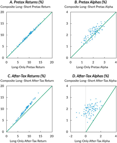
Whereas pretax returns and alphas of the long-only and composite long–short strategies are similar, their after-tax returns differ substantially, as shown in Panels C and D. The composite strategy outperformed the long-only strategy in all 100 simulations after taxes.

Table 1 summarizes the distribution of the annualized returns and alphas across the 100 simulations. The pretax return for the long-only strategy averaged 9.5% per year and ranged between 1.3% and 16.6% across the 100 simulations. The alphas exhibited a lower dispersion because most of the variation in simulated returns resulted from changes in the market returns. The LO pretax alphas averaged 2.0% per year and ranged between 1.0% and 3.2% across simulations.

Table 1. Distribution of Pretax and After-Tax Returns and Alphas across Simulations

	Returns				Alphas
	Long-Only	Composite Long–Short	Difference		Long-Only	Composite Long–Short	Difference
Pretax
Mean	9.5%	9.7%	0.2%		2.0%	2.2%	0.2%
Std. dev.	2.9	2.9	0.3		0.5	0.5	0.3
Minimum	1.3	1.2	–0.4		1.0	1.0	–0.4
Median	9.8	10.0	0.2		2.0	2.3	0.2
Maximum	16.6	17.1	0.9		3.2	3.3	0.9
Proportion positive	100.0	100.0	77.0		100.0	100.0	75.0
Taxes
Mean	–1.4%	–0.2%	1.1%		–1.4%	–0.2%	1.1%
Std. dev.	0.5	0.1	0.5		0.5	0.1	0.5
Minimum	–2.6	–0.5	–0.1		–2.6	–0.5	–0.1
Median	–1.5	–0.2	1.2		–1.5	–0.2	1.2
Maximum	–0.3	0.0	2.4		–0.3	0.0	2.4
Proportion positive	0.0	0.0	99.0		0.0	0.0	99.0
After tax
Mean	8.1%	9.4%	1.3%		0.6%	1.9%	1.3%
Std. dev.	2.4	2.9	0.6		0.7	0.4	0.6
Minimum	0.9	1.0	0.1		–1.2	0.8	0.1
Median	8.4	9.8	1.3		0.6	2.0	1.3
Maximum	14.0	17.0	3.0		2.1	2.9	2.9
Proportion positive	100.0	100.0	100.0		84.0	100.0	100.0

Table 1 also indicates that the combined long– short portfolio was slightly superior to the long-only implementation. The average pretax return for the CLS strategy was 0.2% per year higher than the corresponding return for the LO strategy. In fact, the return of the CLS strategy exceeds the return of the LO strategy in 77 out of the 100 simulations. This difference in pretax returns occurs because the composite strategy enables the investor to implement negative views of stocks. The weights of a long-only strategy are constrained at zero, but a composite long–short strategy can implement negative weights on stocks with negative factor exposures.

Although the pretax performance difference between the two strategies is small, the average after-tax outperformance for the composite strategy relative to the long-only strategy is substantial at 1.3% per year, as shown in Table 1. This significant tax benefit occurs because the necessary turnover of a long-only strategy realizes taxable capital gains on both the market exposure and the active exposure. The passive component in our simulation was assumed to have minimal turnover. Thus, the composite strategy realizes taxable capital gains only on the active long–short component.

Figure 2 shows the distribution of average tax costs for the two strategies across 100 simulated return histories. The lines depict ordinary least-squares (OLS) regressions of average tax costs on average returns and alphas. Panel A shows that the tax costs of the long-only strategy are almost always higher than the tax costs of the composite long–short strategy. Furthermore, the tax costs of the LO strategy increase strongly with the strategy returns, whereas the tax costs of the CLS strategy decrease slightly as strategy returns increase.

Figure 2. Relationship between Pretax Returns and Tax Costs

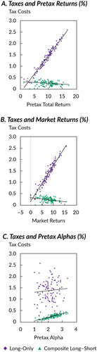
Panels B and C show a decomposition of the strategies’ total returns into market and alpha components. Panel B documents that the positive relationship between total returns and tax costs for the LO strategy is a direct result of the taxation of the aggregate market return. This result is an unintended consequence of the rebalancing of an actively managed long-only strategy. Panel C shows that the tax costs increase for both strategies with the magnitude of the alpha. The reason is that both strategies realize gains on the alpha component through active turnover. The long-only strategy has a substantially higher level of tax costs, however, because it also incurs taxes on the market exposure. Furthermore, whereas the tax costs of the CLS strategy are closely associated with the level of alpha, as is evidenced by the clustering of the tax costs around the regression line, the tax costs of the LO strategy have a high dispersion around the regression line. The tax costs of the CLS strategy are primarily driven by factor performance, and the tax costs of the LO strategy are mostly driven by market performance.¹¹

These results provide evidence that strategies that separate alpha from beta have significant tax benefits when compared with strategies that combine alpha and beta in one long-only portfolio. The composite strategies in which alpha and beta portfolios are managed separately enable the deferral of taxes on the passive market component and allow the rebalancing of the active alpha factor– driven component to take advantage of time-varying factor exposures without generating unnecessary tax costs. Because the tax benefits of separating alpha from beta are robust across simulations, in the remainder of this section, we report solely the average realizations across the 100 simulations .

Different Turnover.

On the one hand, high turnover enables an investment strategy to closely mirror the performance of an ideal factor-based portfolio and to thereby take advantage of favorable factor returns. On the other hand, high turnover can create a significant tax burden because high-turnover strategies tend to exhibit a high propensity to realize capital gains. Strategies that allocate separately to a passive investment in the market portfolio and an actively managed long–short portfolio mitigate the punitive tax consequences of active management because the turnover incurred by the long–short component does not affect the passive component.

Figure 3 depicts the alphas before and after taxes for the long-only and composite long–short strategies. The reported turnover is two-sided turnover that includes establishment and liquidation of portfolio positions; it is reported as a percentage of portfolio NAV.

Figure 3. Relationship between Turnover and Alpha

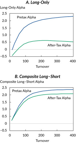
Panel A shows that the pretax performance of the LO strategy increases monotonically with the turnover as a result of superior implementation of the factor exposures. The after-tax alpha for the LO strategy is significantly lower than the pretax alpha, and the gap widens as the turnover increases. At a turnover of around 200% a year, the after-tax alpha of the LO strategy is maximized.

Panel B shows that the tax burden for the CLS strategy also increases with the turnover. The tax burden of the composite strategy is drastically smaller, however, than that of the LO strategy at all turnover levels. The maximum after-tax alpha for the composite strategy is reached at a turnover of around 350%. A stark difference is visible in the magnitudes of maximum after-tax alpha for the LO and CLS strategies: The maximum after-tax alpha of the LO strategy is 62 bps, whereas the maximum after-tax alpha of the CLS strategy is 206 bps. Most of the improvement comes from the higher tax efficiency of the composite strategy.

Table 2 summarizes the performance of the two strategies at different turnover levels. At the base-case turnover of 180%, the pretax information ratio (IR), defined as the ratio of the active return to the active risk of a portfolio, is higher for the composite strategy than for the long-only strategy (0.94 vs. 0.83) because of the superior implementation of the value/momentum factor views. The higher IR for the composite strategy arises from both a slight increase in the pretax alpha and a slight reduction in the active risk. The increase in the pretax return occurs because the implementation of negative views in the composite strategy is not limited by short-selling constraints. The decrease in active risk occurs because the long–short strategy enables a superior diversification of company-specific risks.

Table 2. Performance at Various Turnover Levels

	90% Turnover			180% Turnover			360% Turnover
	LO	CLS		LO	CLS		LO	CLS
Active return
Pretax	1.5%	1.7%		2.0%	2.2%		2.3%	2.3%
Taxes	– 1.1	– 0.2		– 1.4	– 0.2		– 1.7	– 0.3
After tax	0.4	1.5		0.6	1.9		0.5	2.1
Active risk
Pretax	2.0%	2.3%		2.4%	2.3%		2.6%	2.3%
After tax	2.0	2.3		2.4	2.3		2.7	2.3
Information ratio
Pretax	0.74	0.73		0.83	0.94		0.87	1.00
After tax	0.18	0.65		0.25	0.84		0.21	0.90

The advantage of the composite strategy is substantially magnified after taxes. At the base-case turnover of 180%, the IR after taxes equals 0.84 for the composite strategy and just 0.25 for the long-only strategy. This difference occurs because the alpha for the LO strategy is significantly reduced after taxes. In contrast, separating alpha from beta allows investors to dynamically adjust their alpha-driven positions without exposing themselves to unnecessary taxes on their market exposure.

Table 2 also shows the performance of the two strategies at various turnover levels. The pretax IR for both strategies improves with increasing turnover because higher-turnover portfolios enable a better implementation of the factor exposures. The difference between the after-tax IRs of the two strategies grows with the turnover, from 0.47 at a 90% turnover to 0.59 at a 180% turnover and to 0.69 at a 360% turnover. The reason is that the turnover is used efficiently by the CLS strategy to rebalance only the factor exposures but used inefficiently by the LO strategy, where the factor-related turnover affects both factor and market exposures.

Different Market Returns.

We assumed for our base case an average market return of 8%. Table 3 illustrates how the tax burden changes with different average market returns. At a turnover of 180% and an average market return of 0%, both the long-only and the composite long –short strategies generate tax costs of 0.3% per year. In this case, the tax burden is primarily driven by the factor returns. The tax burden of the LO strategy increases from 0.3% at an average market return of 0% to 2.0% at an average market return of 12%. In contrast, the tax burden of the CLS strategy decreases slightly from 0.3% to 0.2% at the same market return levels.¹²

Table 3. Taxes at Different Average Market Return Levels

Average Market Return	90% Turnover			180% Turnover			360% Turnover
	LO	CLS		LO	CLS		LO	CLS
0%	–0.2%	–0.2%		–0.3%	–0.3%		–0.4%	–0.3%
4%	–0.6	–0.2		–0.8	–0.3		–1.0	–0.3
8%	–1.1	–0.2		–1.4	–0.2		–1.7	–0.3
12%	–1.7	–0.2		–2.0	–0.2		–2.5	–0.2

Table 3 illustrates another important aspect of the tax inefficiency of the LO strategy. An interaction effect between turnover and average market return occurs. Specifically, the tax costs of long-only strategies are particularly punitive if those strategies require a high turnover and if the market return is high. For example, if the average market return is 0%, a 90% turnover LO strategy generates tax costs of 0.2% and a 360% turnover strategy generates only slightly higher tax costs of 0.4%. When the average market return is 12%, however, the tax costs of the LO strategy jump from 1.7% at a 90% turnover to 2.5% at a 360% turnover. In contrast, the composite long–short strategy is largely immune to such interaction effects: The tax costs of the CLS strategy vary in a narrow range between 0.2% and 0.3% across different levels of market return and strategy turnover.

Different Factor Returns.

The average factor return in our base-case specification was set at 2% per year. Table 4 summarizes the performance measures of the two strategies —the long-only strategy and the composite long–short strategy—for various levels of factor returns ranging between −2% and +2%. These returns can also be interpreted as manager-specific investment skill.

Table 4. Performance at Various Factor Return Levels

	Factor Return = –2%			Factor Return = 0%			Factor Return = 2%
Metric	LO	CLS		LO	CLS		LO	CLS
Active return
Pretax	–2.0%	–2.1%		0.0%	0.0%		2.0%	2.2%
Taxes	–0.8	0.0		–1.1	0.0		–1.4	–0.2
After tax	–2.7	–2.1		–1.1	0.0		0.6	1.9
Active risk
Pretax	2.3%	2.2%		2.4%	2.3%		2.4%	2.3%
After tax	2.3	2.2		2.4	2.3		2.4	2.3
Information ratio
Pretax	– 0.85	– 0.96		– 0.01	0.00		0.83	0.94
After tax	– 1.16	– 0.96		– 0.45	0.00		0.25	0.84
Turnover	180%	180%		180%	180%		180%	180%

As Table 4 shows, even with an average factor return of −2% a year, the LO strategy still generates tax costs of 0.8% a year. This finding can be explained by the fact that the active return of around −2% is more than offset by the positive return on the market portfolio of around 8%, so the strategy continues to realize capital gains as a result of the market appreciation. The CLS strategy, however, realizes almost no taxable capital gains because it insulates the well-performing passive portfolio from the turnover of the active strategy.

Different Tax Scenarios.

Table 5 shows four alternative tax scenarios in addition to the base case. For these alternatives, we used the base-case assumptions about market and factor return distributions and the active strategy turnover level. The first row restates our base-case results. The second row uses 2019 top tax bracket rates.¹³ The third row assumes a uniform tax rate on all capital gains to indicate how much of the benefit of alpha–beta separation results from the difference between short-term and long-term tax rates. The fourth row assumes that all the tax losses are used immediately to offset capital gains of the same category, which is different from the other scenarios, for which we assumed that losses were carried forward. For example, for the results shown in the fourth row, if the strategy realized a short-term loss and a long-term gain, the short-term loss was assumed to offset short-term gains from other, unrelated investments rather than to offset the long-term gain of the strategy. The assumption for the last row was that the long–short component of the composite strategy was managed by an open-end mutual fund. This assumption led to two significant disadvantages from a tax perspective. First, long–short mutual funds might implement their strategies by trading single equity swaps rather than physical equities because of asset coverage requirements.¹⁴ Assuming that profits on single equity swaps are treated (electively and conservatively) as mark- to-market ordinary income, a mutual fund will pay all its annual profits each year as ordinary dividends. Second, although mutual funds can carry forward capital losses indefinitely, they cannot carry forward ordinary losses.¹⁵

Table 5. Tax Benefits in Different Tax Rate Scenarios

Tax Assumption	LO	CLS
Base-case tax rates (short-term = 35%, long-term = 23.8%)	–1.4%	–0.2%
2019 tax rates (short-term = 40.8%, long-term = 23.8%)	–1.6%	–0.3%
Uniform tax rate (short-term = 20%, long-term = 20%)	–1.3%	–0.2%
Offset of capital gains of the same category	–1.0%	0.3%
Open-end mutual fund	–1.4%	–0.9%

Table 5 shows that in all the tax rate scenarios, the composite long–short strategy has a lower tax cost than the long-only strategy—even when the long –short component has a mutual fund structure.

Manager Termination.

The conventional view is that switching asset managers may have significant tax consequences because the new manager often desires to hold different positions from those held by the old manager, resulting in at least a partial liquidation of old positions and realization of gains accumulated in those positions. Because of these taxes triggered by manager changes, investors may be reluctant to switch managers and thus may be effectively locked into their manager allocations (see, e.g., Holt and Shelton 1962; Stein and Narasimhan 1999; and Lucas and Sanz 2016).

On one end of the spectrum, a very tax-inefficient manager, who realizes most of a strategy’s gains, has high ongoing tax costs but a relatively low tax on termination. On the other end, a very tax-efficient manager, who defers most of the strategy’s gains, has low ongoing tax costs but a relatively high tax on termination. We found that the composite approach allows investors to effectively “have their cake and eat it too.” A strategy that separates alpha from beta enables investors to liquidate only the active component of the portfolio and continue the deferral of capital gains taxes on the tax-efficient passive component. Furthermore, if a market-neutral manager’s termination occurs in response to poor absolute performance, liquidating the active component may provide tax benefits resulting from the realization of capital losses.

Table 6 illustrates the tax consequences of manager termination at various horizons of up to 25 years for the two strategies. Negative values correspond to tax costs, and positive values correspond to tax benefits. We assumed that the manager termination required a complete liquidation of all positions for a long-only strategy and a complete liquidation of the long–short active component for the composite long –short strategy. Because the passive component of the CLS strategy was unaffected by a manager change, it was not liquidated. To evaluate the tax implications of such manager terminations, we multiplied the short-term capital gain or loss realizations as a result of a manager change by the short-term rate and the long-term capital gain or loss by the long-term rate.

Table 6. Tax Consequences of Manager Termination at Various Horizons

Investment Horizon (years)		Factor Return = –2%			Factor Return = 0%			Factor Return = 2%
		LO	CLS		LO	CLS		LO	CLS
5		–0.5%	3.7%		–1.7%	0.9%		–2.6%	–1.6%
10		–1.1	4.6		–2.3	0.5		–3.2	–2.5
20		–0.5	4.8		–2.0	–0.3		–3.0	–2.7
25		–0.7	4.5		–2.3	–0.3		–3.3	–2.5

We focus this discussion on the outcomes shown in Table 6 corresponding to a factor return of –2% because manager termination is more likely for poorly performing managers. Note that the tax costs of a manager termination after a 10-year investment period amount to 1.1% for the long-only strategy. The termination of such a poorly performing manager still causes tax costs because the return of the market exceeds the underperformance of the fund manager. In contrast, the termination of a poorly performing long–short manager after 10 years results in a tax benefit of 4.6% because the passive component of the portfolio is insulated from the active component. The tax implications of manager turnover are qualitatively similar at the different investment horizons because the LO manager is tax inefficient. Manager termination is particularly costly in the case of tax-efficient managers because of their propensity to accumulate substantial unrealized gains. The important finding here, however, is that, even for tax-inefficient managers, a substantial difference in termination tax costs exists between the two strategies.

The differences in tax implications between the long-only and composite long–short strategies decrease as manager ability increases. Nevertheless, the CLS strategy generates lower tax costs than the LO strategy, even if the active manager has a positive pretax alpha. For example, Table 6 shows that the tax costs amount to 3.2% for the LO strategy and 2.5% for the CLS strategy if a manager with a 2% alpha is terminated after 10 years.

Liquidation Taxes.

In the previous subsection, we measured the costs of active manager termination. In this subsection, we report results for the case in which we assumed that the investment was fully liquidated—that is, the liquidation included the passive component of the composite strategy, resulting in the realization of deferred capital gains.

In our analysis, we assumed that no capital gains were realized in the investor’s portfolio outside our strategy. As a result, all the net capital losses were carried forward to future years in their character as either long-term or short-term. For example, in environments of negative expected factor returns, the CLS strategy tended to realize more losses than gains and, as a result, accumulated significant loss carryforwards over time. The liquidation tax liabilities or benefits of a strategy might vary significantly depending on the specific situation of the investor (e.g., the existence of current or expected tax liabilities from other strategies) and the investment vehicle used to manage the strategy. If the strategy is managed in a separate account, carryforward losses remain with the investor to be used to offset current and future capital gains, including gains realized as a result of liquidation. If the strategy is managed by a limited partnership, a complex set of laws, regulations, and practices applies to the liquidation of an investor’s interest.¹⁶ An investor who sells shares of a mutual fund pays tax on the appreciation of those shares without being exposed either to taxes resulting from the fund’s liquidation of securities or to the fund’s carryforward losses.

For simplicity, we reduced these various possible scenarios to two cases. In the first case, we assumed that all the losses of our simulated strategy, including carryforward losses, could be netted against gains of the same character from other investments at the time of liquidation. In other words, long-term capital losses of the strategy (if such existed) were netted with long-term capital gains from other sources and short-term capital losses of the strategy (if such existed) were netted with short-term capital gains from other sources. In the second case, the investor could not benefit from net capital loss realizations. Thus, all the realized net losses, including any remaining loss carryforwards at the time of liquidation, were ignored, but taxes on net gains were paid at the applicable long-term or short-term rates. This scenario might occur if, for example, the investor passed away shortly after liquidating the portfolio, because capital losses cannot be carried forward to future generations.

Figure 4 depicts the cumulative values of the two strategies, assuming that they were completely liquidated after 25 years. In Panels A and B, the expected factor return in this simulation was set at –2.0%. Panel A considers the case of using all the losses in their character to offset gains from other strategies; Panel B considers the case in which all the losses at the time of liquidation are ignored. In the first case, an initial investment of $1 accumulates to $2.95 for the long-only strategy and to $3.20 for the composite long–short strategy. The change in after-tax values during the last month primarily reflects the liquidation taxes. The CLS strategy exhibits a liquidation tax of 12.2% during the last month, whereas the LO strategy exhibits a liquidation tax of only 0.7%. The liquidation taxes are substantially larger for the CLS strategy because it deferred the taxation of most of the market return. Despite the substantially higher liquidation taxes, the composite strategy compounds to a higher after-tax value than the long-only strategy. As shown in Panel B, even in the case where all the liquidation losses are ignored, the CLS strategy accumulates to $3.11, a higher value than the LO strategy. In the cases depicted in Panels A and B, the relative tax efficiency of the composite strategy leaves more capital available for reinvestment, leading to faster wealth accumulation.

Figure 4. Average Simulated Cumulative Portfolio Values with Liquidation

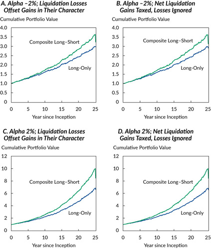
As Panels C and D of Figure 4 show, the effect of faster wealth accumulation (in this case, 2% alpha) is more pronounced when the strategies are more profitable because of the higher alpha. In the full-loss-utilization case shown in Panel C, $1 invested appreciated after liquidation taxes to $6.60 for the long-only strategy and to $8.43 for the composite long–short strategy. Note that the CLS strategy yielded around a one-quarter improvement in value over the LO strategy, even though the deferred gains on the passive component were realized. The liquidation tax for the CLS strategy amounted to 16.8%, whereas the liquidation tax for the LO strategy amounted to only 3.3%. The results were very similar if we ignored losses, as summarized in Panel D.

Results with Management Fees and Transaction and Financing Costs.

In this subsection, we report our investigation of how our results were affected by management fees and transaction costs. We made the following assumptions about fees: For the long-only strategy, we used a fixed fee (inclusive of administrative and other expenses) of 55 bps. This fee level corresponds to the 2018 asset-weighted average expense ratio of equity mutual funds as reported by the Investment Company Institute (ICI 2019).¹⁷ For the composite long–short strategy, we assumed a 10 bp fixed fee on the passive component and the following fees on the active long–short side: a 50 bp fixed fee (inclusive of administrative and other expenses) and a 20% performance fee charged on alpha net of transaction costs, financing costs, and a fixed fee.¹⁸

For transaction costs, we used the estimates in Frazzini, Israel, and Moskowitz (2015). They estimated that the average market impact cost for a large institutional investor managing quantitative strategies in the large-cap developed-markets universe was less than 20 bps of the trading value over the period between 1998 and 2013. Such market impact costs correspond to average trade sizes of around $500,000, amounting to about 1% of a stock’s average daily trading volume. We assumed that transaction costs were 20 bps per dollar traded. For example, using the 20 bp estimate results in 36 bps of annual transaction costs at an annual turnover of 180% of NAV.

For the costs of leverage, following Sorensen, Shi, Hua, and Qian (2007) and Sialm and Sosner (2018), we assumed financing costs of 100 bps per unit of leverage. So, for a long–short portfolio with a leverage of 50% corresponding to a gross notional value of 100%, the financing costs were estimated at 50 bps (i.e., 0.5 × 100 bps).

Finally, we assumed that none of the costs and fees were tax deductible and that they simply reduced the pretax returns. The tax deductibility of fees is a complex topic—especially for partnerships and separately managed accounts—that is beyond the scope of this article. ¹⁹

Although individual investors might encounter significantly higher transaction and financing costs when investing on their own, they are likely to get an exposure to the systematic strategies described in this article through either a commingled vehicle (for example, an open-end mutual fund or a hedge fund) or a separate account managed by a professional manager.

Table 7 reports performance results of the strategies after fees, transaction costs, and taxes at three turnover levels. The pretax gross- of-costs-and-fees results are identical to those shown in Table 2. The trading costs amount to 36 bps per year for both the long-only and composite long–short strategies at a turnover of 180%. Transaction costs increase proportionally with the turnover of the strategies. Whereas transaction costs affect both strategies equally, financing costs are incurred only by the composite long–short strategy. Financing costs reduce the pretax returns for the CLS strategy below the pretax returns of the LO strategy.

Table 7. Performance Net of Fees, Trading Costs, and Financing Costs

	90% Turnover			180% Turnover			360% Turnover
Metric	LO	CLS		LO	CLS		LO	CLS
Active return
Pretax, gross	1.5%	1.7%		2.0%	2.2%		2.3%	2.3%
Transaction costs	–0.2	–0.2		–0.4	–0.4		–0.7	–0.7
Financing costs	0.0	–0.5		0.0	–0.5		0.0	–0.5
Fees	–0.6	–0.7		–0.6	–0.8		–0.6	–0.7
Pretax, net	0.8	0.3		1.1	0.6		1.0	0.4
Taxes	–1.1%	–0.2%		–1.4%	–0.2%		–1.7%	–0.3%
After tax, net	–0.4	0.1		–0.3	0.3		–0.7	0.1
Active risk
Pretax	2.0%	2.3%		2.4%	2.3%		2.6%	2.3%
After tax	2.0	2.3		2.4	2.3		2.7	2.3
Information ratio
Pretax, net	0.38	0.13		0.45	0.24		0.38	0.17
After tax, net	– 0.18	0.04		– 0.12	0.14		– 0.27	0.05

The fees of the long-only strategy are 55 bps; the fees of the composite strategy, which include 10 bps for the passive index component and 60–70 bps for the long–short component, amount to 70–80 bps. The higher fees reduce the pretax attractiveness of the CLS strategy as compared with the LO strategy. Because of the significant tax savings, however, which vary between 0.9% and 1.4%, depending on the strategy turnover, the CLS strategy exhibits substantially higher performance after taxes, fees, and costs than the LO strategy.

Table 7 also shows that the IR net of all the expenses for both strategies is highest at a turnover of around 180%. Not surprisingly, because transaction costs are accounted for in Table 7, the results in that table look different from those in Table 2, where the gross IR continues to increase with turnover. Nonetheless, fees and trading and financing costs do not qualitatively affect the conclusions of our study: The composite long–short strategy has significant tax benefits relative to a long-only strategy with similar factor exposures.

These results also relate to the insight of Siegel, Waring, and Scanlan (2009) that investors should pay active fees for alpha exposure and index fees for beta exposure. A separation of alpha from beta can also, therefore, increase the transparency of the fee structure of asset managers.

Performance of Strategies in Historical Data Simulations

The benefit of Monte Carlo simulations is the ability of the analyst to vary return distribution parameters one at a time and observe their effects on the after-tax performance of the strategies. Modeling the strategies with real data, however, captures the full richness of historical stock returns, including different market regimes, time-varying factor premiums, and fluctuations in the level and dispersion of stock-specific risk.

In this section, we report our tests of whether the main conclusions we reached when we used Monte Carlo simulations remained valid if we instead used historical data. In particular, we asked whether, for the period tested, (1) separating alpha from beta yielded a tax benefit, (2) the tax benefit of separation increased with the level of the market return, and (3) the tax benefit of separation increased with turnover.

Our data were for a US large-capitalization stock universe similar to the Russell 1000 Index and spanned the period 1985–2018.

Methodology.

With real historical data, our portfolio construction methodology closely followed Sialm and Sosner (2018). The optimized portfolio construction allowed us to maintain the same level of active risk through different risk regimes—something that we did not need to worry about with simulated returns drawn from fixed distributions. Thus, our active returns were directly comparable over a long history. In addition, this approach allowed us to introduce tax awareness without changing the key parameters of the strategy (such as active risk, leverage, and turnover), which makes the comparison of tax-aware and tax-agnostic strategies more natural. Details of the methodology are provided in Appendix B.

We used monthly returns and rebalanced our portfolios monthly. Our universe of large-cap US stocks (approximately corresponding to the Russell 1000) excluded REITs, IPO stocks (for 18 months), and multiple share classes of the same company (we retained only the largest market-cap share class).

We constrained the two-sided turnover of the strategies to 180% of portfolio NAV and targeted an active risk of 2%. These levels of risk and turnover closely correspond to our Monte Carlo simulations. In addition, to match the leverage of the long–short component of the composite strategy, we targeted leverage of 50% long and 50% short.

For comparability with the long-only strategy constructed with the universe similar to the Russell 1000, for the passive component of the composite strategy, we replicated the Russell 1000 with the assumption that this investment distributes only dividends, no capital gains, as would likely be the case for an ETF.

Dividends on long positions were treated as qualified dividend income taxed at 20%, and in lieu dividends on the short positions were treated as an expense that could be offset by any type of investment income, including ordinary income and short-term capital gains.²⁰

To calculate tax costs, we applied the same methodology as in the base-case Monte Carlo results. We also used the same assumptions about transaction and financing costs and management fees as in the previous section.

Main Results.

The first two data columns of Table 8 show the historical strategy simulation results in a format similar to that of Table 7. The main result for our purposes is that the tax benefit of separating alpha from beta is 1.2%— similar to what we found in Monte Carlo simulations.

Table 8. Performance of Tax-Agnostic and Tax-Aware Strategies in Historical Simulations, 1985–2018

	Tax-Agnostic Strategy			Tax-Aware Strategy
Metric	LO	CLS		LO	CLS
Active return
Pretax, gross	1.3%	2.0%		1.2%	1.9%
Transaction costs	–0.4	–0.4		–0.3	–0.4
Cost of leverage	0.0	–0.5		0.0	–0.5
Fees	–0.6	–0.7		–0.6	–0.7
Pretax, net	0.4	0.4		0.3	0.4
Taxes	–1.5%	–0.3%		–0.8%	0.0%
After tax, net of costs	–1.1	0.2		–0.5	0.3
Active risk
Pretax	2.1%	2.3%		2.1%	2.3%
After tax	2.1	2.3		2.1	2.3
Information ratio
Pretax, net	0.18	0.19		0.14	0.16
After tax, net	–0.53	0.07		–0.23	0.15
Realization of gains and losses in excess of benchmark
Long-term capital gains (losses)	4.7%	3.0%		5.3%	3.5%
Short-term capital gains (losses)	0.9	–2.2		–1.9	–5.5
All capital gains (losses)	5.6	0.8		3.4	–2.0
Portfolio characteristics
Annual turnover, % of NAV	180%	182%		169%	182%
Gross notional value, % of NAV	100	195		100	195
Active leverage, % of NAV	97	95		95	95

As the bottom panel of Table 8 shows, not only do the active risk levels of the long-only and composite long–short strategies closely match but also their turnover and active leverage—the sum of absolute active weights —are virtually identical. Despite this close match in the high-level strategy characteristics, the CLS strategy achieves a gross pretax alpha, as shown in the final column, that is significantly higher than that of the LO strategy. The reason for this difference in alpha is the ability of the CLS strategy to implement factor signals more efficiently than the LO strategy, as discussed by Clarke, de Silva, and Thorley (2002, 2006). As a result, when we implemented a realistic optimized portfolio construction in the historical simulations, the separation of alpha from beta improved both pretax and after-tax returns—even when management fees and trading and financing costs were accounted for. Because the purpose of our study was to analyze the tax benefits of alpha –beta separation, however, we continue to focus on tax results rather than on the potential pretax benefits of the separation.

Sialm and Sosner (2018) showed that tax awareness can significantly reduce the tax burdens of both long-only and long–short strategies. Our optimized portfolio construction allowed us to easily introduce tax awareness while holding constant other portfolio characteristics —such as target turnover, leverage, and active risk. The results for the tax-aware strategy are shown in the last two columns of Table 8. For the LO strategy, tax awareness reduced the tax cost from 1.5% to 0.8%. For the CLS strategy, the tax cost was reduced from 0.3% to zero. The reason the tax-aware CLS strategy did not realize a tax benefit as in Sialm and Sosner (2018) is that we made the assumption that losses were carried forward. Sialm and Sosner assumed that losses could be used immediately to offset gains from other, unrelated investments. The modeling of tax-aware strategies in addition to tax-agnostic strategies shows that, although the LO strategy obtains substantial benefits from tax awareness, the CLS strategy still has significantly lower tax costs than the LO strategy. Moreover, we found that even the tax-agnostic CLS strategy had a lower tax cost than the tax-aware LO strategy (0.3% compared with 0.8%) and a meaningfully higher after-tax net-of-fees-and-costs alpha (0.2% compared with –0.5%).

Different Tax Scenarios.

As in our Monte Carlo simulations, we tested the robustness of our historical simulation results to different tax rate assumptions. Table 9 shows that for all considered tax treatments, the composite long–short strategy resulted in substantially lower tax costs than the long-only strategy. The tax results in Table 9 for historical data are qualitatively and quantitatively similar to the tax results in Table 5 that we obtained using Monte Carlo simulations. In addition, the CLS strategy realized substantially higher after-tax returns than the LO strategy.

Table 9. Tax Benefits in Various Tax Scenarios in Historical Simulations, 1985–2018

Metric	LO	CLS
Active return
Pretax, gross	1.3%	2.0%
Transaction costs	–0.4	–0.4
Cost of leverage	0.0	–0.5
Fees	–0.6	–0.7
Pretax, net	0.4	0.4
Taxes in various tax scenarios
Base-case tax rates (short-term = 35%, long-term = 23.8%)	–1.5%	–0.3%
2019 tax rates (short-term = 40.8%, long-term = 23.8%)	–1.7	–0.3
Uniform tax rate (short-term = 20%, long-term = 20%)	–1.2	–0.3
Offset capital gains of the same category	–1.3	0.3
Open-end mutual fund	–1.5	–0.7
After-tax net return in different tax scenarios
Base-case tax rates (short-term = 35%, long-term = 23.8%)	–1.1%	0.2%
2019 tax rates (short-term = 40.8%, long-term = 23.8%)	–1.3	0.1
Uniform tax rate (short-term = 20%, long-term = 20%)	–0.8	0.2
Offset capital gains of the same category	–0.9	0.7
Open-end mutual fund	–1.1	–0.3

The Tax Benefits of Separating Alpha and Beta for Various Levels of Market Return.

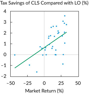
Our Monte Carlo simulations showed that the tax benefits of alpha–beta separation increase with the level of the average market return. Although we have only one return history, during which the average market return was 11.5%, we can still test the prediction that the tax benefits of separation will vary positively with the market return. Figure 5 plots for the 34 years in our sample the relationship between annual market return and tax savings resulting from the separation. We also plot the univariate OLS regression line. The slope of the line is highly significant with a t-statistic of 3.8.

Figure 5. Relationship between Market Return and Tax Savings for the CLS Strategy Compared with the LO Strategy in Historical Data Simulations, 1985– 2018

The Tax Benefits of Alpha–Beta Separation and Strategy Turnover.

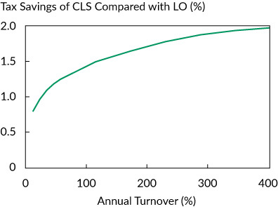
In our historical sample period, the market return was high and positive; therefore, according to our Monte Carlo simulations, the historical simulations should exhibit a strong positive relationship between strategy turnover and the tax benefit of separating alpha from beta. We varied target turnover over a wide range and plotted the results for our strategies in Figure 6. The historical strategy simulation is consistent with Monte Carlo simulations shown in Figure 3: The tax benefits of separation increase with turnover.

Figure 6. Relationship between Annual Turnover and Tax Savings for the CLS Strategy Compared with the LO Strategy in Historical Data Simulations, 1985–2018

Conclusions

Commonly offered advice for taxable investors is to stay away from actively managed strategies. The rationale in favor of passive investing is that any extra pretax returns achieved through active management might not be enough to compensate the investor for the associated tax costs. Our results show that the average alpha of a long-only strategy decreases from 2.0% before taxes to 0.6% after taxes. Thus, taxes have a significant impact on after-tax portfolio returns. After transaction costs, fees, and taxes are taken into account, the alpha of a long-only strategy is, on average, negative. According to our estimates (which are consistent for the Monte Carlo and historical data simulations), a long-only manager’s gross pretax alpha needs to be as high as 2.3%–2.4% to overcome all the costs.

We have presented an approach that significantly reduces the tax burden of active strategies by separating alpha and beta exposures. Importantly, our approach is effective even when an investor has access only to tax-agnostic strategies. As a result, our approach is a practical solution to tax efficiency in a world dominated by tax-agnostic managers.

We compared the after-tax performance of the traditional approach of expressing views on stocks via a long-only strategy with that of an alternative approach where such views are expressed as a market-natural long–short strategy while the market exposure is implemented via a separate passively managed portfolio. The traditional approach combines alpha and beta, whereas our alternative approach separates them.

We first tested our strategies in Monte Carlo simulations where we controlled the levels of both the market return and the active strategy return. This approach allowed us to arrive at general conclusions that did not depend on the market’s performance or the performance of various actively managed strategies over a given sample period. We then complemented our Monte Carlo analysis by using real, historical data.

Our main conclusion is that for a taxable investor, separating alpha from beta is beneficial. Separate exposure to market-neutral long–short alpha strategies and passive beta indexes allows taxable investors to defer gains on market appreciation and thus significantly reduce their tax costs. This conclusion is robust to the level of market return, an active strategy’s alpha and turnover, various tax rate assumptions, management fees and transaction and financing costs, and the tax costs of strategy liquidation.

Finally, we considered the tax costs of manager replacement. Our results show that an ability to replace only the alpha manager without changing the beta exposure results in significant tax benefits. Those benefits are particularly large in a realistic scenario —that is, when an active manager is replaced as a result of poor performance.

Acknowledgment

We are grateful for the comments and suggestions of Michele Aghassi, CFA, Phil Balzafiore, Stephen Brown, Daniel Giamouridis, Pete Hecht, Lukasz Pomorski, Ted Pyne, Scott Richardson, Benjamin Schneider, CFA, Stathis Tompaidis, one anonymous referee, and the participants at the 2017 AQR Capital Management Research Conference.

Notes

¹ Clarke, de Silva, and Thorley (2009) provided a comprehensive analysis of the pretax costs and benefits of separating alpha from beta. They did not discuss the tax consequences of this separation.

² See, for example, Israel and Moskowitz (2012); Vadlamudi and Bouchey (2014); Santodomingo, Nemtchinov, and Li (2016); Ehling, Gallmeyer, Srivastava, Tompaidis, and Yang (2018); Sialm and Sosner (2018); and Goldberg, Hand, and Cai (2019).

³ See, for example, Gallmeyer, Kaniel, and Tompaidis (2006); Berkin and Luck (2010); Sialm and Sosner (2018); and Sosner, Krasner, and Pyne (2019).

⁴ Individual investors and small family offices might be de facto constrained in their ability to short directly in their accounts. For such investors, commingled vehicles managing long–short market-neutral strategies might be a practical solution for separating alpha from beta. Although tax-efficient wrappers such as insurance dedicated funds are available in the market, a significant portion of private wealth is invested through taxable accounts.

⁵ See Ang (2014) for a general discussion of factor investing.

⁶ The assumption of 2% average return and 4% volatility for the value and momentum factors implies an information ratio of 0.5. In simulations not reported here, we increased the volatility of these factors to 6% and then to 8% while holding the average return at the 2% level. We found that the tax benefits of separating alpha from beta are virtually identical for alternative factor volatilities in the 4%–8% range.

⁷ The –0.7 correlation is more negative than the correlation between the Fama and French value (high book to market minus low book to market, or HML) and momentum (up minus down, or UMD) factors, which are available on Kenneth French’s website ( https://mba.tuck.dartmouth.edu/pages/faculty/ken.french/data_library.html). Our value factor exposures were based on the most recent price, following Asness and Frazzini (2013) and Asness et al. (2013), rather than the lagged price as in Fama and French (1993). The correlation between the Asness–Frazzini version of HML and the Fama–French UMD is –0.7. In simulations not reported here, we found similar results using correlations ranging between –0.4 and –0.7.

⁸ The tax rates of 35% on short-term gains and 20% on long-term gains correspond approximately to the average tax rates of investment income over recent decades in the United States. These rates are slightly lower than the top federal marginal investment tax rates in the United States in 2019, which were 23.8% for long-term gains and 40.8% for short-term gains (including the 3.8% net investment income tax under IRC Section 1411). IRC Section 1222 defines the holding periods for the determination of long-term and short-term capital gains and losses, and IRC Section 1 provides the applicable tax rates for short-term and long-term capital gains. Note that many states impose additional taxes on capital gains, which are not included in these rates. Unless explicitly stated, we assumed that the strategies invested in physical stocks, not in equity swaps. We also assumed that the investment funds had not made the IRC Section 475(f) mark-to-market ordinary election. For physical stocks, gains and losses are generally taxed at the time of realization (IRC Section 1001) and evolve from short-term to long-term when a position is held for more than one year (IRC Section 1222). We used these rules of stock taxation in our modeling.

⁹ See Dickson, Shoven, and Sialm (2000); Berkin and Ye (2003); and Israel and Moskowitz (2012) for a discussion of accounting methods for the tax lot selection.

¹⁰ The capital gains netting and carryforward rules are governed by, respectively, IRC Sections 1222 and 1212(b). In our simulations, we did not incorporate the fact that investors can annually subtract capital losses of up to $3,000 from their ordinary income.

¹¹ Our results were not affected qualitatively by using alternative investment strategies based on value, momentum, or short-term reversal.

¹² The CLS strategy was required to reduce the size of the long–short component after a poor market performance to maintain the desired balance between the passive and active portfolios. Such partial liquidations can trigger the realization of taxable capital gains. In contrast, in an increasing market, a combined strategy can simply expand both the long and the short positions of the active component, which does not cause capital gains realizations.

¹³ In 2019, under IRC Section 1, the top-bracket federal tax rates for short-term and long-term capital gains were 37% and 20%, respectively. In addition, a net investment income tax of 3.8% was imposed under IRC Section 1411.

¹⁴ Section 18 (“Capital Structure”) of the Investment Company Act of 1940.

¹⁵ IRC Section 852(b)(2)(B).

¹⁶ See Sosner, Balzafiore, and Du (2018) for a brief description of some of the partnership taxation rules. A discussion of the tax consequences of liquidating partnership interests is outside the scope of this article.

¹⁷ The value-weighted expense ratio of equity mutual funds in 2018 amounted to 0.55%, whereas the equal-weighted expense ratio amounted to 1.26%, according to the 2019 ICI Factbook (ICI 2019), p. 120.

¹⁸ The fee for the passive index approximates the gross expense ratio of the SPDR S&P 500 ETF (traded under the ticker symbol SPY), which is the largest and most liquid ETF as of this writing. The long–short fee is derived from the data in the Hedge Fund Research (HFR) database ( www.hedgefundresearch.com/hfr-database). The 70 funds that composed the HFR Equity Market Neutral Index as of June 2019 exhibit asset-weighted and equal-weighted management fixed fees of, respectively, 112 bps and 135 bps and performance fees of, respectively, 16.8% and 18.3%. These funds are not directly comparable, however, to the long–short fund we modeled in our study. We targeted an active risk of 2%, whereas the equity market-neutral funds in the HFR database are run at a much higher risk level. The performance fee mechanically reflects this low level of risk, and we simply rounded up the performance fee to 20%. The management fixed fee requires an adjustment, however, for the lower level of risk. To estimate the risk of the funds, we used the 55 funds that had at least 36 months of returns. We then computed the annualized volatility of net-of-fee returns for each fund. The asset-weighted and equal-weighted average annualized return volatilities of these funds were, respectively, 6.8% and 7.9%. Because the returns are net of fees, and performance fees reduce return volatility, it is plausible that an average hedge fund in the HFR database targets 8% or higher gross-of-fees risk. At a 2% target risk, the appropriate management fixed fee should be a quarter of the fee of the funds in the HFR database, or approximately 30 bps. Adding to this fee other administrative costs and fund expenses and rounding up, we obtained the fixed fee estimate of 50 bps.

¹⁹ Sosner, Pyne, and Chandra (2019) discussed some of the complexities related to fee deductibility in the light of the Tax Cuts and Jobs Act of 2017.

²⁰ See Sialm and Sosner (2018) for further details about the treatment of long-term and short-term dividends and specific tax code sections that sanction that treatment.

²¹ Our universe was different from the Russell 1000 for the following reasons: (1) REITs were excluded because they are often considered a distinct asset class; (2) stocks that had an IPO within the last 18 months were also excluded; and (3) for companies with multiple share classes, we retained only the share class with the largest market cap.

²² Israel, Liberman, Sosner, and Wang (2019) found that dividend avoidance has a negative impact on after-tax expected returns.

Appendix A.

Monte Carlo Simulation Methodology

Factor Signals.

We analyzed a three-factor model with a market factor, a value factor, and a momentum factor. We simulated monthly returns from a multifactor distribution for 500 stocks. The vector of cross-sectional stock returns for month t, r_t, is defined as $r_t=X_t{f}_t+{\epsilon }_t,$(A1) where X_t is the matrix of stock-level factor exposures at time t, f_t is the realization of factor returns at time t, and ${\epsilon }_t$ is the vector of stock-specific returns at time t. Factor return realizations are jointly normally distributed with a time-invariant vector of mean returns µ and a time-invariant return covariance matrix F:

$f_t\sim N\left(\mu ,F\right).$(A2)

The idiosyncratic returns of the stocks were assumed to be uncorrelated and to come from an independent normal distribution with a mean of zero and a variance of ${\sigma }^2$ for each stock i:

${\epsilon }_{i,t}\sim N\left(0,{\sigma }^2\right).$(A3)

We assumed that all the returns were price returns and ignored dividend payments. Hence, our simulated strategy generated only capital gains, no dividend income.

The first column of the exposure matrix X_t represents market betas. The market betas were assumed to be constant over time and to equal 1.0 for all stocks. The exposures to the three style factors were computed as follows: At the end of month t for each stock i, we computed the exposure of stock i to style j. We began by defining raw style signals as $s_{i,j,t}={\theta }_j{\displaystyle \sum _{h=t-K_j+1}^{t-L_j}{}_{\epsilon i,h}},$(A4) where ${}_{\epsilon i,h}$ is a stock-specific return of stock i in month h and the set of parameters $\left\{{\theta }_j,K_{j,}{L}_j\right\}$ defines the investment style j—value (V) or momentum (M). The parameter ${\theta }_j$ captures the sign of the signals, and the parameters K_j and L_j capture the lag structure of the signals. The value signal depends inversely on the idiosyncratic returns over the prior 60 months (i.e., ${\theta }_V=-1$, $K_V=60$, and $L_V=0$). The momentum signal depends positively on the idiosyncratic performance of a stock over the prior 12 months excluding the most recent month (i.e., ${\theta }_M=1$, $K_M=12$, and $L_M=1$).

To obtain style factor exposures as of the end of month t, we ranked the raw signals $s_{i,j,t}$ from the lowest to the highest, where a stock with the lowest rank is the least attractive according to the signal and a stock with the highest rank is the most attractive. The ranks were then demeaned and standardized in the cross section to obtain the factor exposures $x_{i,j,t}$ that determined style factor–related stock returns in month t + 1.

Portfolio Formation.

We constructed long-only and long–short portfolios on the basis of total stock returns. This total return–based portfolio construction methodology is plausible because investors and portfolio managers generally observe total returns. For each individual style factor, using returns as defined by the multifactor model, we computed the style signals at the end of month t as follows:

$q_{i,j,t}={\theta }_j{\displaystyle \sum _{h=t-K_j+1}^{t-L_j}{r}_{i,h}.}$(A5)

The sets of parameters $\left\{{\theta }_j,K_j,L_j\right\}$ are as defined in the previous section: ${\theta }_V=-1,K_V=60,$ and $L_V=0$ for value; and ${\theta }_M=1,K_M=12,$ and $L_M=1$ for momentum.

The raw signals for a given style portfolio were ranked from the lowest to the highest. The ranks were then demeaned. Subsequently, value and momentum demeaned ranks were combined with equal weights, and the combined signal was ranked and demeaned again. For the long-only strategies, only positive demeaned ranks were used as weights; for the long–short strategies, both positive and negative demeaned ranks were used. For comparability of the results, both long-only and long–short strategy weights were rescaled to the gross notional value of 1.0 so that the long-only strategy weights added up to 100% and the long–short strategy was 50% long and 50% short. We refer to such weights as v_i,t, where i stands for a stock and t stands for the month when the weights were constructed.

The weights for the long-only and long–short strategies were updated monthly, resulting in a potentially large turnover. To scale turnover to more realistic levels, we smoothed the strategy weights by averaging the current weights prescribed by the preceding process. That is, for each stock i, we computed the grown portfolio weight as $g{w}_{i,t}=w_{i,t-1}\left(1+r_{i,t}\right),$(A6) where $w_{i,t-1}$ is the previous period’s weight of stock i and $r_{i,t}$ is the return of stock i during month t.

We rescaled these grown weights to the gross notional value of 1.0 to get grown rescaled weights h_i,t (long-only to sum up to 100% and long–short to sum up to 50% long and 50% short). Then, we computed the smoothed weights as a weighted average of these grown rescaled weights and the current weights v_i,t derived from stock rankings:

${\tilde{w}}_{i,t}=\lambda h_{i,t}+\left(1-\lambda \right)v_{i,t}.$(A7)

We then performed a final rescaling of ${\tilde{w}}_{i,t}$ to sum to 100% for long-only strategies and to 50% long and 50% short for long– short strategies. The initial smoothed weights ${\tilde{w}}_{i,0}$ were set equal to the initial unsmoothed weights (i.e.,$$ ${\tilde{w}}_{i,0}=v_{i,0}$). We iteratively calibrated the smoothing coefficient λ every month so that the turnover as a percentage of NAV was 180%.

Appendix B.

Historical Simulation Methodology

The methodology we used when using historical data closely followed Sialm and Sosner (2018). We focus here on a quantitative strategy that combined the value and momentum style factors.

Alpha Model.

We began the portfolio construction process with an alpha model that yielded stock-level alphas. Black and Litterman (1992) showed that alpha forecasts consistent with risk and correlation forecasts are more effective in portfolio optimization. Jones, Lim, and Zangari (2007) adapted this insight to factor investing in the context of equity portfolios. We used their methodology to obtain stock-level alphas because our tax-aware approach relies on optimization to achieve a balance between the pretax alpha and the tax costs of portfolio rebalancing.

The starting point for our alpha forecasts was a model portfolio, $\tilde{v}$, which is long attractive stocks and short unattractive stocks. The determination of relative attractiveness for each factor in the model—in our case, value and momentum—was done at the end of every calendar month with data available at that time. The model portfolio $\tilde{v}$ is a vector of long–short portfolio weights that captures the combined exposures of stocks to value and momentum factors. For example, stocks with high value and momentum exposures exhibit positive weights, whereas stocks with low value and momentum exposures exhibit negative weights.

Following the methodology of Jones et al. (2007), at every month-end, we converted the model portfolio into a vector of stock-level alphas by multiplying it by the stock-level covariance matrix $\Sigma$ from MSCI Barra’s USE3L risk model (discussed in more detail later in the appendix):

$\alpha =\Sigma \tilde{v}.$(B1)

The alpha forecasts used in the optimization relied on only the information available at the time of portfolio construction.

Model Portfolio Construction.

We constructed factor-based model portfolio $\tilde{v}$ as follows: We first constructed long–short value and momentum factor portfolios within a US large-cap stock universe that approximately corresponded to the Russell 1000.²¹

For our measure of value, we used the book-to-market ratio, in which the denominator was the most recently available market cap (Asness and Frazzini 2013). Book values came from the Compustat annual files. We lagged the annual book values by six months relative to the fiscal year-end to ensure that they were available at the time of model construction. For our measure of momentum, we used the total return over the past 12 months excluding the most recent month.

The book-to-market and momentum raw scores were then turned into industry-relative ranks. For the industry classification, we used the industry levels of the Global Industry Classification Standard developed by MSCI and Standard & Poor’s. We ranked the stocks within each industry according to their book-to-market and momentum scores. These ranks within each industry were demeaned (by subtracting the average rank within an industry) and standardized (by dividing by the standard deviation of the ranks within an industry) to create an industry-neutral portfolio. Because the weights of a portfolio summed to zero within each industry, the weights of the whole portfolio also summed to zero. These long –short portfolio weights for the two signals are denoted here by $v_{VAL}$ for value and $v_{MOM}$ for momentum. This rank-based portfolio formation method is similar to that of Asness, Ilmanen, Israel, and Moskowitz (2015).

The value and momentum portfolios were then normalized by their respective volatility forecasts:

${\tilde{v}}_{VAL}=\frac{1}{{\sigma }_{VAL}}{v}_{VAL}$(B2)

and

${\tilde{v}}_{MOM}=\frac{1}{{\sigma }_{MOM}}{v}_{MO\mathrm{M.}}$$$(B3)

Using a covariance matrix produced by the MSCI Barra USE3L risk model, we computed the volatility forecasts. The risk model yielded a stock-level covariance matrix every month. We used this covariance matrix, $\Sigma$, lagged by one month, to compute ${\sigma }_{VAL}$ and ${\sigma }_{MOM}$ as follows:

$\begin{array}{c}{\sigma }_{VAL}=\sqrt{{v^{\prime }}_{VAL}\Sigma v_{VAL}}\\ \end{array}$(B4) $\text{and}$${\sigma }_{MOM}=\sqrt{{v^{\prime }}_{MOM}\Sigma v_{MO\mathrm{M.}}}$$$(B5)

Lagging the covariance matrix by one month accounts for the fact that it takes a few days after the month-end for the risk model to be released, and it ensures that the covariance matrix used in the volatility calculations was available at the time of factor portfolio formation.

The model portfolio was then constructed as an equal-weighted average of the value and momentum portfolios:

$$v=\frac{1}{2}{\tilde{v}}_{VAL}+\frac{1}{2}{\tilde{v}}_{MOM}.$$(B6)

Finally, the model was normalized by its predicted volatility:

$\tilde{v}=\frac{1}{\sigma }v.$(B7)

The model volatility, σ, was computed in the same way as the value and momentum factor volatilities.

Covariance Matrix.

Similar to Asness et al. (2015), we used covariance matrixes from MSCI Barra, which applies a multifactor approach to covariance matrix estimation. The MSCI Barra USE3L risk model provides a covariance matrix of all stocks traded on US exchanges. The model uses 52 industries and 13 risk factors—including volatility, size, value, momentum, and leverage—to capture the common variation in stock returns. The model is updated monthly from information about stock returns and fundamentals available at month-end.

Similar to the Fama and MacBeth (1973) procedure, our model first used past data to compute factor loadings and then estimated cross-sectional regressions of stock-level returns on those factor loadings. The regression coefficients estimated in each period are factor returns for that period, and the regression residuals are stock-specific returns for that period. Time-series factor returns up to that period were then used to compute a forward-looking forecast of the factor covariance matrix. Stock-specific returns up to that period were used to compute forward-looking stock-specific volatility forecasts. More details about the model estimation are available in the model handbook (Barra 1998).

Portfolio Construction.

Using stock-level alpha and covariance matrix estimates, we constructed long-only and long–short portfolios, which we updated every month-end. The portfolio weights of the individual securities in long-only strategies were all positive and summed to 100%. For the long-only portfolios, the betas relative to the Russell 1000 were constrained to be close to 1.0. The weights of a long–short portfolio summed to zero. The betas of the long–short portfolios relative to the Russell 1000 were constrained to be close to zero. Longs and shorts of the long–short portfolio were limited to 50% of the NAV each. Thus, the long–short portfolio’s gross notional value could not exceed 100% of the NAV.

Note that optimization allowed us to construct both tax-agnostic and tax-aware strategies. Tax awareness was implemented through a penalty term that incorporated tax costs into the portfolio’s objective function.

The optimization problem for the long-only strategy was defined as follows:$\underset{w_1\dots w_N}{\max }{\displaystyle {\sum }_i{w}_i{\alpha }_i-\gamma T}$(B8) subject to${\displaystyle {\sum }_i{\displaystyle {\sum }_j{w}_i{w}_j{\sigma }_{ij}\le T{E}^2}}$ ${\displaystyle {\sum }_i\left(b_i+w_i\right)=1}$ $0.98\le {\displaystyle {\sum }_i\left(b_i+w_i\right){\beta }_i\le 1.02}$ ${\displaystyle {\sum }_i\left|w_i-w_{i,0}\right|}\le 1.8,$ where w_i and α_i correspond to the active portfolio weight and the alpha of security i, γ is the tax aversion coefficient (equal to zero for tax-agnostic optimization and 0.1 for tax-aware optimization), T is the tax cost of rebalancing the portfolio in the current period, c is transaction costs, ${\sigma }_{ij}$ is the covariance between the returns of securities i and j derived from MSCI Barra’s risk model, TE is the target tracking error of 2% annually, b_i is the benchmark weight of security i, β_i corresponds to the beta of security i with respect to the Russell 1000 predicted by the MSCI Barra risk model, and w_i,0 corresponds to the pre-rebalance weight of security i, which was used to set a constraint on the strategy’s turnover.

For the long–short strategy, the weights were not defined relative to a benchmark; thus, the optimization problem was defined slightly differently:$$\underset{w_1\dots w_N}{\max }{\displaystyle {\sum }_i{w}_i{\alpha }_i}-\gamma T-c$$(B9) subject to${\displaystyle {\sum }_i{\displaystyle {\sum }_j{w}_i{w}_j{\sigma }_{ij}\le R^2}}$ ${\displaystyle {\sum }_i{w}_i}=0$ $-0.02\le {\displaystyle {\sum }_i{w}_i{\beta }_i\le 0.02}$ ${\displaystyle {\sum }_i\left|w_i-w_{i,0}\right|\le 1.8}$ ${\displaystyle {\sum }_i{w}_i^{+}\le 0.5,{\displaystyle {\sum }_i\left|w_i^{-}\right|}}\le 0.5,$where R is the target risk level of 2% annually for the long–short portfolio and $w_i^{+}$ and $w_i^{-}$ denote positive and negative portfolio weights that defined leverage constraints.

The tax cost of rebalancing a portfolio was defined as $T=t_{LT}{g}_{LT}+t_{ST}{g}_{ST},$(B10) where t_LT and t_ST are, respectively, the long- and short-term capital gain tax rates, and g_LT and g_ST are, respectively, the net long-term and short-term capital gains computed from individual tax lots. The tax burden, T, is expressed as a proportion of the strategy’s NAV. Although dividend taxes and in lieu short dividend deductions were not explicitly incorporated into the optimization, they are included in the reported after-tax returns.²² Unrealized gains were also not included in the optimization problem. We used the HIFO tax lot accounting method throughout this article.

References

- Ang, A.. 2014. Asset Management: A Systematic Approach to Factor Investing. New York: Oxford University Press https://doi.org/10.1093/acprof:oso/9780199959327.001.0001.
- Arnott, R.D., V.Kalesnik, and T.Schuesler. 2018. “Is Your Alpha Big Enough to Cover Its Taxes? A Quarter-Century Retrospective.” Journal of Portfolio Management, vol. 44, no. 5: 78–102 https://doi.org/10.3905/jpm.2018.44.5.078.
- Asness, C.S., and A.Frazzini. 2013. “The Devil in HML’s Details.” Journal of Portfolio Management, vol. 39, no. 4: 49–68 https://doi.org/10.3905/jpm.2013.39.4.049.
- Asness, C.S., A.Ilmanen, R.Israel, and T.J.Moskowitz. 2015. “Investing with Style.” Journal of Investment Management, vol. 13, no. 1: 27–63.
- Asness, C.S., T.J.Moskowitz, and L.H.Pedersen. 2013. “Value and Momentum Everywhere.” Journal of Finance, vol. 68, no. 3: 929–85 https://doi.org/10.1111/jofi.12021.
- Barra. 1998. United States Equity: Version 3 (E3) Barra Risk Model HandbookNew York: Barra.
- Bergstresser, D., and J.Pontiff. 2013. “Investment Taxation and Portfolio Performance.” Journal of Public Economics, vol. 97: 245–57 https://doi.org/10.1016/j.jpubeco.2012.04.005.
- Bergstresser, D., and J.Poterba. 2002. “Do After-Tax Returns Affect Mutual Fund Inflows?” Journal of Financial Economics, vol. 63: 381–414 https://doi.org/10.1016/S0304-405X(02)00066-1.
- Berkin, A.L., and C.G.Luck. 2010. “Having Your Cake and Eating It Too: The Before- and After-Tax Efficiencies of an Extended Equity Mandate.” Financial Analysts Journal, vol. 66, no. 4: 33–45 https://doi.org/10.2469/faj.v66.n4.3.
- Berkin, A.L., and J.Ye. 2003. “Tax Management, Loss Harvesting, and HIFO Accounting.” Financial Analysts Journal, vol. 59, no. 4: 91–102 https://doi.org/10.2469/faj.v59.n4.2548.
- Black, F., and R.Litterman. 1992. “Global Portfolio Optimization.” Financial Analysts Journal, vol. 48, no. 5: 28–43 https://doi.org/10.2469/faj.v48.n5.28.
- Clarke, R., H.de Silva, and S.Thorley. 2002. “Portfolio Constraints and the Fundamental Law of Active Management.” Financial Analysts Journal, vol. 58, no. 5: 48–66 https://doi.org/10.2469/faj.v58.n5.2468.
- Clarke, R., H.de Silva, and S.Thorley. 2006. “The Fundamental Law of Active Portfolio Management.” Journal of Investment Management, vol. 4, no. 3: 54–72.
- Clarke, R., H.de Silva, and S.Thorley. 2009. Investing Separately in Alpha and Beta. Charlottesville, VA: Research Foundation of CFA Institute.
- Dickson, J.M., and J.B.Shoven. 1995. “Taxation and Mutual Funds: An Investor Perspective.” Tax Policy and the Economy, vol. 9: 151–80 https://doi.org/10.1086/tpe.9.20061830.
- Dickson, J.M., J.B.Shoven, and C.Sialm. 2000. “Tax Externalities of Equity Mutual Funds.” National Tax Journal, vol. 53: 607–28 https://doi.org/10.17310/ntj.2000.3S.01.
- Edelen, R., R.Evans, and G.Kadlec. 2013. “Shedding Light on ‘Invisible’ Costs: Trading Costs and Mutual Fund Performance.” Financial Analysts Journal, vol. 69, no. 1: 33–44 https://doi.org/10.2469/faj.v69.n1.6.
- Ehling, P., M.Gallmeyer, S.Srivastava, S.Tompaidis, and C.Yang. 2018. “Portfolio Tax Trading with Carryover Losses.” Management Science, vol. 64, no. 9: 4156–76 https://doi.org/10.1287/mnsc.2017.2733.
- Fama, E.F., and K.R.French. 1993. “Common Risk Factors in the Returns on Stocks and Bonds.” Journal of Financial Economics, vol. 33, no. 1: 3–56 https://doi.org/10.1016/0304-405X(93)90023-5.
- Fama, E.F., and J.D.MacBeth. 1973. “Risk, Return, and Equilibrium: Empirical Tests.” Journal of Political Economy, vol. 81, no. 3: 607–36 https://doi.org/10.1086/260061.
- Frazzini, A., R.Israel, and T.J.Moskowitz. 2015. “Trading Costs of Asset Pricing Anomalies.” Working paper. http://faculty.som.yale.edu/Tobiasmoskowitz/documents/TradingCostofAssetPricingAnomalies.pdf.
- Gallmeyer, M., R.Kaniel, and S.Tompaidis. 2006. “Tax Management Strategies with Multiple Risky Assets.” Journal of Financial Economics, vol. 80, no. 2: 243–91 https://doi.org/10.1016/j.jfineco.2004.08.010.
- Goldberg, L.R., P.Hand, and T.Cai. 2019. “Tax-Managed Factor Strategies.” Financial Analysts Journal, vol. 75, no. 2: 79–90 https://doi.org/10.1080/0015198X.2019.1567191.
- Holt, C., and J.Shelton. 1962. “The Lock-In Effect of the Capital Gains Tax.” National Tax Journal, vol. 15: 337–52.
- ICI. 2019. 2019 Investment Company Factbook: A Review of Trends and Activities in the Investment Company Industry59th ed.Washington, DC: Investment Company Institute www.ici.org/pdf/2019_factbook.pdf.
- Israel, R., J.Liberman, N.Sosner, and L.Wang. 2019. “Should Taxable Investors Shun Dividends?” Journal of Wealth Management, vol. 22, no. 3: 49–69 https://doi.org/10.3905/jwm.2019.1.080.
- Israel, R., and T.J.Moskowitz. 2012. “How Tax Efficient Are Equity Styles?” Working paper.
- Israel, R., T.J.Moskowitz, A.Ross, and L.Serban. 2017. “Implementing Momentum: What Have We Learned?” Working paper.
- Jeffrey, R.H., and R.D.Arnott. 1993. “Is Your Alpha Big Enough to Cover Its Taxes?” Journal of Portfolio Management, vol. 19, no. 3: 15–25 https://doi.org/10.3905/jpm.1993.710867.
- Jones, R., T.Lim, and P.J.Zangari. 2007. “The Black–Litterman Model for Structured Equity Portfolios.” Journal of Portfolio Management, vol. 33, no. 2: 24–33 https://doi.org/10.3905/jpm.2007.674791.
- Lucas, S., and A.Sanz. 2016. “Pick Your Battles: The Intersection of Investment Strategy, Tax, and Compounding Returns.” Journal of Wealth Management, vol. 19, no. 2: 9–16 https://doi.org/10.3905/jwm.2016.19.2.009.
- Means, K.. 2002. “A Proposal for Tax-Efficient Active Equity Investing: Active Long Portfolio = Index Portfolio + Market Neutral Portfolio.” Journal of Wealth Management, vol. 5, no. 3: 57–66 https://doi.org/10.3905/jwm.2002.320456.
- Santodomingo, R., V.Nemtchinov, and T.Li. 2016. “Tax Management of Factor-Based Portfolios.” Journal of Index Investing, vol. 7, no. 2: 78–86 https://doi.org/10.3905/jii.2016.7.2.078.
- Sialm, C., and N.Sosner. 2018. “Taxes, Shorting, and Active Management.” Financial Analysts Journal, vol. 74, no. 1: 88–107 https://doi.org/10.2469/faj.v74.n1.1.
- Sialm, C., and H.Zhang Forthcoming. “Tax-Efficient Asset Management: Evidence from Equity Mutual Funds.” Journal of Finance.
- Siegel, L.B., M.B.Waring, and M.H.Scanlan. 2009. “Five Principles to Hold Onto (Even When Your Boss Says the Opposite).” Journal of Portfolio Management, vol. 35, no. 2: 25–41 https://doi.org/10.3905/JPM.2009.35.2.025.
- Sorensen, E.H., J.Shi, R.Hua, and E.Qian. 2007. “Aspects of Constrained Long–Short Equity Portfolios.” Journal of Portfolio Management, vol. 33, no. 2: 12–20 https://doi.org/10.3905/jpm.2007.674790.
- Sosner, N., P.Balzafiore, and Z.Du. 2018. “Partnership Allocations and Their Effects on Tax-Aware Fund Investors.” Journal of Wealth Management, vol. 21, no. 1: 8–17 https://doi.org/10.3905/jwm.2018.21.1.008.
- Sosner, N., S.Krasner, and T.Pyne. 2019. “The Tax Benefits of Relaxing the Long-Only Constraint: Do They Come from Character or Deferral?” Journal of Wealth Management, vol. 21, no. 4: 10–31.
- Sosner, N., T.Pyne, and S.Chandra. 2019. “Understanding the Tax Efficiency of Relaxed-Constraint Equity Strategies.” Working paper, AQR Capital Management.
- Stein, D.M., and P.Narasimhan. 1999. “Of Passive and Active Equity Portfolios in the Presence of Taxes.” Journal of Private Portfolio Management, vol. 2, no. 2: 55–63 https://doi.org/10.3905/jwm.1999.320359.
- Vadlamudi, H., and P.Bouchey. 2014. “Is Smart Beta Still Smart after Taxes?” Journal of Portfolio Management, vol. 40, no. 4: 123–34 https://doi.org/10.3905/jpm.2014.40.4.123.