Evolutionary Finance for Multi-Asset Investors

Abstract

Standard strategic asset allocation procedures usually neglect market interaction. However, returns are not generated in a vacuum but the result of the market’s price discovery mechanism. Evolutionary finance accounts for this and endogenizes asset prices.

This paper develops a multi-asset evolutionary finance model. Requiring little more than dividend and interest rate data, it provides a valuable guide to this class of models. While traditional mean/variance optimization is concerned with finding the optimal allocation, evolutionary finance’s focus is on finding the optimal strategy. This paper shows that yield-based strategies outperform competing alternatives and are evolutionarily advantageous for multi-asset investors.

Keywords:

• evolutionary finance
• multi-asset
• portfolio choice
• strategic asset allocation

PL Credits: 2.0:

Introduction

Evolutionary finance studies financial markets using concepts rooted in biology. Investment strategies compete for market share and only the best survives—finance’s equivalent to the “survival of the fittest” popularized by Darwin (1869).

In nature, many interactions and dependencies exist. Foxes decimate rabbits until there are too few of them to feed the many foxes at which point the population of rabbits starts growing again. A finance parallel might be momentum strategies that invest until prices have moved so far away from fundamentals that value investors’ approach becomes profitable again and the market is pushed in the opposite direction.

Evolutionary portfolio theory puts these ideas to work in the realms of portfolio choice. Most importantly, it allows prices to be determined within the model, which is certainly one of its most exciting features. Moreover, in the traditional asset allocation literature, the interaction between investment strategies is little studied. However, especially for big multi-asset investors such as sovereign wealth funds or large pension plans, their actions (e.g., asset allocation changes) have the potential to move prices. Moreover, even small occupational pension plans often follow very similar investment strategies and their collective impact can also affect market prices. Therefore, many investors are increasingly concerned with understanding their investment strategy’s impact¹ on financial markets—and whether their investment strategy is set up to be successful, i.e., survives, in the long run. A topical example would also be how the increased adoption of sustainable (ESG) investing might impact returns. Evolutionary finance allows testing one’s strategy with (and against) investment strategies followed by other market participants in a hypothetical environment that might materialize in the future. Moreover, it shifts the strategic asset allocation discussion away from mere optimization towards scenario analyses and an investigation of how a fund’s strategy might assert itself in the market. This paper shows how the mathematical framework of evolutionary portfolio theory can be applied to the decisions faced by multi-asset investors.

A Brief History of Evolutionary Finance

The memorable metaphor of financial markets and biological evolution has led to a lot of interest in evolutionary finance by scholars and practitioners alike²—a field that is based on research in financial economics, game theory and behavioral finance.

In most of the asset allocation and mathematical finance literature, returns are treated as exogenous. This is different in evolutionary finance where returns are endogenous. Indeed, a game theoretic perspective is probably more appropriate—after all, prices and thus returns are generated by trading among investors. Evolutionary finance also introduces dynamics to an otherwise often static asset allocation decision. Another way to accomplish that is to employ for example a vector autoregression approach (e.g., Campbell, Chan, and Viceira 2003; Campbell and Viceira 2005; Hoevenaars et al. 2008) or techniques such as bootstrapping. The main difference to those approaches is that in evolutionary finance, returns are not predicted based on historical data or taken from a distribution but are generated endogenously by trading and market clearing among market participants with different strategies. This paper is therefore also very interesting for decision makers who already employ stochastic models but long for a different perspective that takes market interaction into account. Moreover, the paper provides investors who do not yet have (or do not have licensed) a sophisticated economic scenario generator with a tool to set up a first dynamic piece in their asset allocation process.

Whereas in classic mean/variance optimization, investors search for a mean variance-optimal allocation and that usually at one point in time, evolutionary portfolio theory—which is an application of evolutionary finance to portfolio theory—tries to find an optimal strategy (i.e., a sequence of asset allocations over time) that maximizes relative wealth versus competing strategies. Hence, in an evolutionary finance setting, investing according to mean/variance optimization is one of many possible strategies. Moreover, in evolutionary portfolio theory, the optimization to find the best strategy cannot be executed by any investor individually but is indirectly established through market selection. Another important distinction is that contrary to most portfolio choice models which require an investor’s utility function (which is still a much debated topic, see for example Sharpe (2007) or recently Warren (2019)), this is not the case in evolutionary finance.

The focus in evolutionary portfolio theory is therefore not on utility maximization but on finding the investment strategy that achieves the highest growth rate of wealth (Amir et al. 2021). Indeed, as Sciubba (2006, 125) once aptly put it, this survival strategy “might not make you happy, but will definitely keep you alive.” Research in evolutionary finance includes Farmer (2002), Lo (2004), Evstigneev, Hens, and Schenk-Hoppé (2006), Evstigneev, Hens, and Schenk-Hoppé (2008), Lo (2012), Evstigneev, Hens, and Schenk-Hoppé (2016) and Lo (2017) where usually a model similar to Blume and Easley (1992) forms the analysis’ basis.

Blume and Easley (1992) investigated the market selection mechanism for assets with diagonal payoffs³ and endogenous prices and showed that the surviving investment rule corresponded to “betting your beliefs.” This result had up to then only been proven for exogenous prices and was known at least since Breiman (1961) as investing according to the Kelly (1956) criterion.⁴ However, once also non-diagonal payoffs are allowed, the surviving strategy is no longer a basic Kelly rule which allocates according to the maximization of the expected logarithm of wealth (e.g., based on some total return estimate) but a strategy that invests according to expected relative dividends (Evstigneev, Hens, and Schenk-Hoppé 2006). This paper therefore also provides a link between evolutionary finance and the Kelly (1956)-optimal behavior of a log-utility optimizing investor in classic portfolio theory. Moreover, it not only provides the necessary formulas for a practical application of evolutionary portfolio theory but also includes a written explanation of how to build such a system.

Relative wealth growth was studied by Lo, Orr, and Zhang (2018) and Orr (2018) through the lens of population genetics which lends itself especially to investigating more short-term developments. Indeed, relative wealth is often at least as important as absolute wealth (e.g., Robson 1992 or Bakshi and Chen 1996). Lo, Orr, and Zhang (2018) showed that the Kelly criterion was not always optimal in that case and that the optimal strategy in particular depended on an investor’s initial relative wealth. The robustness check with a dominant starting strategy later in the paper investigates this using different starting wealths.

If rational expectations were introduced again, Sandroni (2000)⁵ and Blume and Easley (2006) showed that expected utility maximizers would ultimately achieve market dominance as a consequence of their most appropriate choice of the savings rate. Of course, scholars have also been interested in how investors with incorrect beliefs affect markets. De Long et al. (1990, 1991) showed that so-called noise traders can deter rational arbitrageurs and drive prices away from their fair value. Similarly, Kogan et al. (2006, 2017) found that even if noise traders’ wealth became negligible, they could still have a price impact.⁶ A variation of this issue is studied as a robustness check in this paper.

Advancements in the field of evolutionary finance have managed to generalize many of these findings and helped bring them closer to a practical application. Where the surviving strategy in Evstigneev, Hens, and Schenk-Hoppé (2006) allocated according to relative dividend amounts (given that they were i.i.d.), Amir et al. (2021) were the first to endogenize asset payoffs by production functions as of market capital and found that the surviving strategy needed to allocate according to the return on equity times market capitalization. As dividends are ultimately a function of a firm’s profitability, this is already much closer to a strategy that could be put into practice for example based on dividend yields. This paper extends and applies that idea to multi-asset investing.

Although this paper’s focus remains on asset-only strategic asset allocation for brevity and clarity, the method could be extended to a case with liabilities where for example the yield resulting from investors’ government bonds trading in the evolutionary model could be used as a discount factor. Similarly, De Giorgi (2008) developed an evolutionary model with liabilities for the case of insurance companies or pensions funds and analytically devised which strategy would avoid bankruptcy almost surely in case of unexpectedly large (i.e., indemnities exceeding collected premia and other income) withdrawals. The evolutionary stable strategy was found to be qualitatively similar to the case without liabilities but invested (much) less wealth into the risky asset (De Giorgi 2008). Hence, the presence of liabilities primarily affects sizing in an evolutionary model.

This paper contributes to the literature in several ways. First, it provides a practical guide to evolutionary finance, its theory and methods. Second, it applies evolutionary portfolio theory to multi-asset investing. Evolutionary finance and multi-asset investing indeed form a natural pair. On the one hand and most importantly, multi-asset investing literally encompasses the whole ecosystem of investments. On the other hand, we are able to abstract from an obstacle in the prevalent stock market analyses. Evolutionary finance models need a payout and at the index level there is almost always some sort of payment to investors. Third, this paper empirically investigates and extends several results that have hitherto only been derived analytically. Finally, using simulations that require little more than (real-life) payouts, it shows that relative yield-based strategies outperform alternative allocation approaches for a broadly diversified sample portfolio comprised of government bonds, corporate bonds, REITs and equities.

Methodology

Evolutionary portfolio theory primarily studies relative wealth shares. The strategy that gathers the highest wealth will ultimately dominate the market. In order to get there, it must earn payouts and achieve capital gains larger than those of competing strategies. Contrary to backtests, returns are determined by the strategies’ interaction within the model.⁷

The key to endogenizing returns is to understand market capitalizations as prices. Suppose a stock currently has a market capitalization of USD 100 m. Now, more investors get attracted to this company’s shares and they (collectively) want to invest USD 10 m while the existing investors wish to retain their position. In order for the market to clear, the company’s market capitalization must rise to USD 110 m. Assuming no new issuances or redemptions,⁸ this (i.e., market clearing) can only be achieved if the share price rises by 10%.

Theory

In terms of notation and model setup, we closely follow Evstigneev, Hens, and Schenk-Hoppé (2016). Evolutionary finance models of this type are based on the work of Lucas (1978) and feature three key equations.

Investors $i=1,\dots ,I$ determine their allocation⁹ ${\alpha }^i$ to strategies $s=1,\dots ,S$ at time t. Strategies allocate a fraction λ to asset classes $k=1,\dots ,K$ according to their weighting scheme (e.g., market capitalization weights). Equation 1 describes an asset's (relative) market capitalization where ω expresses relative wealth either of investors ${\omega }_t^i=\frac{w_t^i}{{\sum }_{i=1}^I{w}_t^i}$ or, what we are ultimately interested in, of strategies ${\omega }_t^s=\frac{w_t^s}{{\sum }_{s=1}^S{w}_t^s}.$ 1 $${\lambda }_t^{M,k}={\sum }_{s=1}^S{\lambda }_t^{s,k}{\omega }_t^s\mathrm{ }\text{where}\mathrm{ }{\omega }_t^s={\sum }_{i=1}^I{\alpha }_t^{i,s}{\omega }_t^i$$1

The return for asset class k can be computed according to Equation (2) with D denoting the dividend or interest payment. 2 $$r_{t+1}^k=\frac{{\lambda }_{t+1}^{M,k}+D_{t+1}^k}{{\lambda }_t^{M,k}}$$2

The evolution of wealth for strategy s is then given by Equation (3). 3 $${\omega }_{t+1}^s={\sum }_{k=1}^K{r}_{t+1}^k{\lambda }_t^{\mathrm{s},k}{\omega }_t^s$$3

Equations (1–3) generate a dynamic stochastic model, i.e., a random dynamical system. This can be expressed in matrix notation as in Equation (4)4 $${\omega }_{t+1}={\left[Id-{\mathit{\Theta }}_t{\mathit{\Lambda }}_t\right]}^{-1}{\mathit{\Theta }}_t{d}_t$$4 and solved using linear programming where Id is the identity matrix, $\Theta$ the matrix of asset holdings (i.e., ${\left[\frac{{\lambda }_t^{s,k}{\omega }_t^s}{{\sum }_{s=1}^S{\lambda }_t^{s,k}{\omega }_t^s}\right]}_s^k$), $\Lambda$ the matrix of allocations and d the scaled payout matrix holding each asset’s relative payout (i.e., $d_{k,t}=\frac{D_{k,t}}{D_t}$). The equation’s first part captures (relative) wealth changes due to capital gains or losses and the second part those due to investment income. 4 $${\omega }_{t+1}={\left[Id-{\mathit{\Theta }}_t{\mathit{\Lambda }}_t\right]}^{-1}{\mathit{\Theta }}_t{d}_t$$4

Hence, strategies determine asset demands. Summing the allocation of all strategies to a particular asset class determines its price¹⁰ at time t. At the end of year t, dividends and interest are paid and investors (through strategies) trade again. The return to a strategy is thus comprised of payouts and ultimately the capital gains or losses (the percentage difference between the summed demand at t and t + 1, be careful to account for payouts only once) it receives on its holdings.

The dividend and interest rate processes were assumed to be exogenous. Moreover, we used payouts (coupons (shifted +1 year) minus credit losses times aggregate face value¹¹ or dividend yields times market capitalization (in USD)) which anchors assets to what they are conceivably able to produce in reality. Dividends and interest rate payments are made from cash earned through operating activities in the economy. Prices in financial markets however are determined by supply and demand for financial assets. Financial markets and the real economy are thus viewed similar to two separate ecosystems. Nevertheless, even if dividends were allowed to increase with market value, for example,¹² a unique evolutionary stable investment strategy can still be identified¹³ (Amir et al. 2021).

Investment Strategies

Contrary to stocks where the most popular strategies are those based on factors (e.g., value), the strategy set is more diverse in the multi-asset domain. On the one hand, it includes virtually every investor and asset class and on the other hand, allocation procedures are often less straightforward. Nevertheless, some strategies are very widely-followed and thus represent a good proxy for the power balance present in the markets.

Neither leverage nor negative weights were allowed. If a strategy were to have allocated a non-positive value to an asset class, that weight was set to zero (should all be zero, we resort to 1/n). Although, we did this to best reflect the practice of multi-asset investing, Amir et al. (2022) found in an extension of the evolutionary finance model to short-selling that strategies with non-positive weights cannot even be survival strategies.

Basic Strategies

These four strategies represent the most popular and time-tested approaches and lay the foundation for this paper’s analysis.

1/n Allocation

Equal weights on all asset classes.

Market-Cap Weighted

Using (endogenous) market capitalization weights after t = 0. Corresponds most closely to passive index investing.

Historical Mean Return

Historical mean (total) returns are a popular source for expected returns in practice and this method allocates according to them. If we had only two assets with US equities having achieved a mean return of 10% and US Treasuries one of 5%, they would get an allocation for the next period of $\frac{10}{10+5}=67\%\mathrm{ }\text{and}\mathrm{ }\frac{5}{10+5}=33\%$ respectively. Realized historical returns were used until the simulation started and from then onwards a blend of those and endogenous ones.

Yield

The current yield for bonds and the dividend yield for equity and REIT indices. The same allocation procedure as for the historical mean return variant was used—just using yields instead of returns (i.e., if US Treasuries offered a yield of 5% and US Equities a dividend yield of 5%, the allocation at that point in time would be 50/50).

Additional Strategies

Adding to the basic strategies and later applied to a more exhaustive asset sample, this section introduces a wider array of multi-asset allocation approaches.

60/40 allocation 60% of the wealth allocated to equities and 40% to bonds. Within the equity and bond portion, allocations were made according to the (simulated) market capitalization. Although a very popular approach especially in the US, it was not included into the basic strategies as its weights were frequently very close to those of the market capitalization allocation. In order to see one dominant strategy emerge, strategies should arguably be as orthogonal as possible (i.e., not hold very similar portfolios) at least for the initial evaluation.

Trailing One-Year Return

This is a proxy for time series momentum and allocates according to the previous year return for each asset class.

Risk-Free Rate plus Historical Excess Return

A sensible way to take the current interest rate environment¹⁴ into account when forecasting returns.

Carry-Based Expected Returns

A strategic asset allocation variant using carry-based expected returns as in Schnetzer (2018). The Yield variant neglects an important difference between the asset classes in this analysis, which is that equity holders are entitled to participate in a firm’s future growth. Hence, this allocation uses proper expected returns which for bonds were computed as the yield-to-worst minus (expanding window) historical credit losses plus the rolldown and for REITs and equities as the dividend yield plus the dividend growth rate. Two allocation procedures were included. One variant allocated simply according to expected returns and the other one based on the expected Sharpe ratio.

Insurance

A proxy for a typical (life) insurer's balance sheet. 50% government bonds, 35% corporate bonds and 7.5% each in real estate and equities (market capitalization-weighted within categories). Since REITs are usually more highly levered than the direct real estate holdings of most insurance companies they are a sensible but of course only imperfect proxy.

Mean/Variance Optimization

Traditional mean/variance optimal weights (MVO) based on the seminal work by Markowitz (1952) using historical (and simulated) mean returns and a shrunk covariance matrix.

Description of the Data Set

The base sample consisted of the Bloomberg Barclays US Treasury index, the Bloomberg Barclays US Corporate Bond index, the US Nareit Equity REIT index and the S&P 500 index. The extended sample added indices for government bonds, corporate bonds and equities in the UK, the Eurozone and Japan as well as US high-yield bonds and the MSCI Emerging Markets equity index.

The time period covers data from 1973 to 2020 with the simulation period starting when the necessary data was first available for all indices, namely in 1974 for the base sample and in 2002 for the extended sample with annual intervals.

All data were retrieved from Bloomberg except where stated otherwise. In particular, our source for credit loss data was Moody's Annual Default Study and data for US REITs were retrieved from the Nareit website.¹⁵

Results

Every year in December, asset allocation was carried out and prices were determined within the system. The base evaluation was restricted to only few but very popular strategies. Figure 1 shows each strategy’s wealth share over time.

Figure 1. Wealth Shares

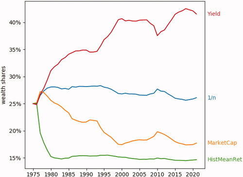
The yield-based strategy outperformed the others in this multi-asset environment, thereby confirming that prior year dividends and interest payments are a good signal for an evolutionary strategy. This also supports a result Evstigneev, Hens, and Schenk-Hoppé (2006) analytically devised for stocks. In particular, the yield-based strategy ate away at the strategy that allocated according to historical returns and the one that was allocated according to market capitalization weights. Simply using past returns was thus not evolutionarily advantageous. Indeed, interest and dividend payments comprise the stable component of total returns and in an evolutionary setting, they ultimately dominate since capital gains are more erratic. Although this sample period was too short for the yield-based strategy to achieve complete dominance (convergence is slow in real life), it is important to note that the more dominant a strategy becomes, the more it also determines prices.

Overall, turnover was low as asset allocation and trading only took place once a year. However, there were of course differences between strategies with the historical return-based strategy exhibiting the highest and the market capitalization-based strategy exhibiting the lowest turnover. These differences are not high enough to break the dominance of the yield-based strategies, which have a turnover in between market capitalization-based strategies and return-based strategies.

More Assets, More Strategies

The main simulation delivered intriguing results but most multi-asset investors have to prove themselves in global markets and against a more diverse set of competing strategies. Hence, the sample was expanded to include a broader and more representative array of asset classes. Moreover, the strategy set was extended to more asset allocation schemes.

Figure 2 depicts the results for this expanded sample.¹⁶

Figure 2. Wealth Shares (More Assets, More Strategies)

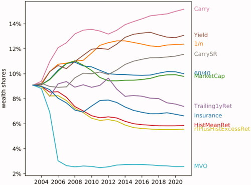
Again, the yield-based strategy achieved a high relative wealth share but was now surpassed by the carry-based strategy. Contrary to the yield-based variant, the carry approach employs a more comprehensive estimate of expected returns. In particular, it extends the equation for equities and REITs by a growth estimate. Also for this expanded strategy set, capital gains-focused approaches were among those that were dominated. A strategy’s relevant factor in a random dynamical system is its growth rate. The intuition behind yield-based strategies’ success can thus be seen as the carry representing the stable component of wealth accumulation. Capital gains on the other hand are noisy and thus evolutionarily fragile. Hence, there always exists a mutant strategy that will able to dominate a capital gains-based strategy.

The biggest disappointment might be the low market share achieved by the mean-variance optimization. However, this might be a consequence of the relatively short period that was available to estimate the covariance matrix which is examined in the robustness checks section. Indeed, despite covariance shrinkage and a no short-selling constraint, it held a particularly heavily concentrated portfolio at the beginning of the simulation period which was much less pronounced in the robustness check with a longer covariance estimation period (and foresight) displayed in Figure 3d later in this paper. Although it was still dominated, its loss in relative wealth share was much more gradual. Allowing it to use an arguably superior expected return estimate such as carry-based expected returns instead of historical returns would have also improved its performance albeit it still finished with the lowest relative wealth share. Moreover, note that even though it was dominated, this need not mean that it lost its investors money in absolute terms. Even the mean/variance optimization achieved a terminal wealth slightly above its starting one (and thus generated a positive annualized return) but it just grew much slower than more evolutionary successful approaches. Additionally, once an investment rule has lost a (large enough) amount of wealth it falls into a state of marginalization (i.e., it does not matter much anymore what the mean-variance optimization strategy achieves in terms of returns). Furthermore, the longer the simulation runs, the more the market is dominated by the surviving strategies which—once have they achieved market dominance alone or as a coherent group—will also determine prices, making it difficult for marginalized strategies to recover. Nevertheless, it is important to note that more evolutionary successful strategies will be able to claw back wealth share as is examined in the robustness check with 50% of the starting wealth allocated to the market capitalization-based strategy. Moreover, the mean-variance optimization strategy has some features of an imitation strategy as it employs realized returns and covariances to determine its asset allocation. Hence, it is also influenced by and learns from the behavior of more evolutionary successful strategies and to some degree also adapts to those. A similar behavior can also be observed from the relative wealth share development of the historical mean-based strategies. Of course, the endogenous returns and those that manifested in reality need not be the same. The mix of realized and simulated returns may thus be a challenge for the mean-variance optimization strategy. Indeed, as the number of endogenous returns in its return and covariance estimation window grows, the asset allocation it generates seems to improve and the strategy slows its wealth share loss. For an investment strategy to become fully extinct however, a much longer time horizon would be needed.

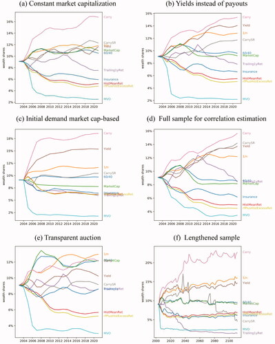
Figure 3. Robustness Checks

Some might be surprised that the volatile year of 2020 did not lead to greater redistributions of wealth. This was a consequence of many firms still having made their 2020 payouts roughly over the amount that was expected (i.e., the argument of remunerating shareholders for and from 2019 profits). Moreover, return volatility tends to decrease over time as the sole source of exogenous variation entering the model is the one in real-life payouts.

Robustness Checks and Variations

Constant Market Capitalization

In order for market capitalizations to correspond to prices, the capital base must stay the same. However, this need not necessarily be the case for indices. For example, the market capitalization of the REIT index has grown substantially over the past decades also because more qualifying securities could be included. In this paper, the payout was determined as yield times (point-in-time) market capitalization. If market capitalization increases simply due to an increasing number of securities, the approximation might not be sufficiently accurate anymore. This robustness check fixed market capitalizations to the value they had in 2002 (the simulation’s start date)¹⁷ and also calculated payouts based on that value. Figure 3a shows that this even increased the most successful payout-based strategy’s lead while it narrowed the distance between the other yield-based ones, the market cap-oriented allocation approaches and the 1/n allocation method.

Yields Instead of USD Payouts

This variant is related to the previous one. Another cure for market cap-agnostic behavior is the use of fixed percentage yields instead of fixed payouts. This is also how most analytical work in evolutionary finance has been done. Although an appealing alternative, its drawback is that an asset class' yield will not decrease at higher prices. Figure 3b depicts the results. Little change was observable to the initial specification.

Initial Demand Market Cap-Based

The main simulation starts by endowing USD 1 to every strategy and letting each one choose the weights according to its specific asset allocation algorithm. However, an alternative would be to assume that the whole world currently invests passively according to market capitalization weights and use those as the starting weights at t = 0. The early points in Figure 3c already show why this solution is not preferable. Such a setup leads to a big price change at t = 1 which then plagues asset allocation approaches that rely on historical returns and/or volatilities over the whole simulation period. On the other hand, this is the only variant where initial (real-life) market capitalizations and strategies’ asset demand are proportional. In any case, the same strategies as in the previous evaluations achieved the highest wealth shares and were therefore evolutionarily superior.

Full Sample for Correlation Estimation

The mean-variance optimization’s dismal performance certainly warrants a closer look given its popularity in practice. It was certainly handicapped by the comparatively short history (three years) available to estimate correlations at sample start. Hence, in this variation, all strategies that required standard deviation or correlation inputs for their asset allocation were allowed to use the entire sample of real-life prices (note that this creates a forward-looking bias). The resulting wealth shares in Figure 3d indeed show that this improved the performance of the mean-variance optimization allocation a bit and that of the Sharpe ratio carry-based approach a lot. However, even despite them having the benefit of using some forward-looking information, they still could not outperform the dominant strategy.

Transparent Auction

In this paper, strategies’ asset demand works similar to them submitting market orders. This can potentially generate large price movements (i.e., slippage) at which investors would maybe no longer be interested in transacting. This variant takes that into account and introduces a price discovery mechanism similar to a transparent (opening) auction. Before actual trading and price determination takes place, investors (i.e., through their strategies) go through five rounds of price negotiation and get the opportunity to adjust their allocation and orders based on the expected clearing price.

Figure 3e shows that this particularly improved the approaches that heavily rely on market capitalizations for their asset allocation. Nevertheless, the carry method as a representative of payout-focused strategies remained in the top group and even started to quickly gain back market share from those strategies. The 60/40 and the market cap allocation also benefited here from their comparable investments. Due to their similar allocation styles, they together have (almost) twice the market power of more orthogonal approaches and can thus quicker reach a state where they can potentially determine prices.

Lengthened Sample Period

Many of the assets in the extended sample have a relatively short data history (∼20 years). As convergence to strategy dominance is relatively slow it would be nice to have a (much) longer evaluation period. This variant simply stacks the same data set 5 times to the original one (always reversed to avoid jumps at joints). This extended version confirmed the main results as is evident from Figure 3f.

However, in particular the Sharpe ratio-based carry version lost a lot of market share towards the middle of the simulated period. One reason was that the Sharpe ratio indeed turned negative for most equity asset classes as dividend growth approached zero over time (i.e., an index with increasing payouts in the main sample will become one with negative dividend growth in a reversed period) and the risk-free rate was higher than the dividend yield leading to no allocation to those assets. A (block) bootstrap analysis will certainly be able to present a more realistic picture.

Bootstrap Analysis

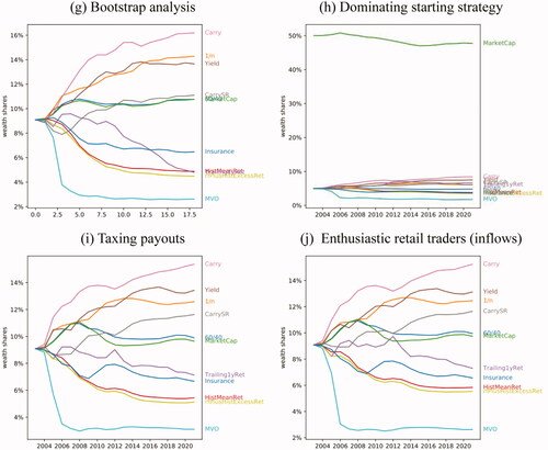
A way to “expand” a data set and investigate it from another perspective is to employ bootstrap analysis. We used the circular block bootstrap of Politis and Romano (1992) and the Politis and White (2004) algorithm¹⁸ to determine the optimal block size. Then, we ran 10 bootstrap iterations and took the average resulting wealth to determine the wealth shares in Figure 3g. This analysis again confirmed the main results.

Dominant Starting Strategy

It could be the case that a dominant strategy can never be pushed out of the market. Hence, this variant endows the market capitalization-based strategic asset allocation which is very popular in practice, an initial relative wealth of 50% (with the other strategies sharing the other half). Figure 3h illustrates that more evolutionary successful strategies will start to eat into the (artificially-set) dominant strategy. However, convergence, as always, is slow.

Taxing Payouts

Yield-based strategies might favor assets with high payout yields which bear a tax disadvantage in most jurisdictions. In this robustness check, payouts were taxed at a (marginal) tax rate of 20%. However, as can be seen in Figure 3i, this did not materially affect the results.

Enthusiastic Retail Traders (Inflows)

So far, we have not assumed any in- or outflows. This variant introduces an outside capital stock (cash) held by retail investors. These investors monitor the strategy that allocates according to trailing one-year returns and if that strategy generated a positive return (i.e., similar to having observed longer-term time series momentum), invest in that strategy. Their collective contribution is 10c in that case (as a reminder, USD 1 was endowed to each strategy at t = 0). Figure 3j shows that these inflows naturally increased the trailing one-year return strategy's wealth share but without being able to challenge the most evolutionary successful strategies’ dominance.

Removing One Strategy

Ultimately, including the relevant strategies is crucial. Although the strategies were carefully chosen with maximum representativeness in mind, it is important to examine how strongly the results depended on the strategy universe.

Table 1 shows that especially the winning (and losing) few strategies did not change substantially if a formerly present asset allocation variant was removed from the sample. Strategic asset allocations based on yields and payouts clearly remained dominant. This also empirically helps confirm the so far most general result in evolutionary finance. Evstigneev et al. (2020) recently derived that for any set of investment strategies and dividend processes the survival strategy was always a contrarian, diversified strategy based on fundamentals.

Table 1. Removing One Strategy

	(1)	(2)	(3)	(4)	(5)	(6)	(7)	(8)	(9)	(10)	(11)
(1) 60/40	–	7	6	6	8	7	7	7	6	6	6
(2) 1/n	8	–	8	8	9	8	8	8	8	8	8
(3) MarketCap	6	6	–	5	7	6	6	6	5	5	5
(4) HistMeanRet	3	3	3	–	5	3	3	3	3	2	3
(5) Trailing1yRet	5	5	5	2	–	5	5	5	2	4	4
(6) Yield	9	9	9	9	6	–	10	9	9	9	9
(7) Carry	10	10	10	10	10	10	–	10	10	10	10
(8) CarrySR	7	8	7	7	3	9	9	–	7	7	7
(9) rfPlusHistExcessRet	2	2	2	3	4	2	2	2	–	1	2
(10) MVO	1	1	1	1	1	1	1	1	1	–	1
(11) Insurance	4	4	4	4	2	4	4	4	4	3	–

Highest rank corresponds to highest terminal wealth.

Sensitivity to Initial Conditions

Table 2 investigates the results’ stability with respect to the conditions that prevailed at the start of the simulation period. Whereas in the former evaluation, the period started in 2002 and lasted until the end of 2020, Table 2 additionally presents the terminal wealth ranking for later simulation start dates. Those strategies that achieved the highest terminal wealths in the main evaluations were usually also those that did so for later starting dates. Moreover, the top places were typically occupied by strategies using fundamentals such as yields as the basis for their asset allocation.

Table 2. Sensitivity to Initial Conditions

	Base	2003	2004	2005	2006	2007	2008	2009	2010
60/40	7	7	7	5	6	6	6	6	6
1/n	9	8	8	10	9	8	7	8	9
MarketCap	6	6	6	3	5	5	5	5	4
HistMeanRet	3	3	4	4	3	4	3	4	2
Trailing1yRet	5	4	3	2	4	1	1	1	3
Yield	10	9	10	11	11	10	9	11	8
Carry	11	11	11	8	10	9	10	9	10
CarrySR	8	10	9	6	8	11	11	10	11
rfPlusHistExcessRet	2	2	2	1	2	2	2	2	1
MVO	1	1	1	9	1	3	8	3	7
Insurance	4	5	5	7	7	7	4	7	5

Highest rank corresponds to highest terminal wealth.

Conclusion

Evolutionary portfolio theory offers a fascinating solution to one of the most prolific problems in asset allocation. By allowing for interaction between investment strategies, it manages to endogenize prices and thereby facilitates a close look at the inner workings of financial markets. Moreover, it presents investors with a tool to test their strategic asset allocation’s prowess in a dynamic and competitive environment.

This paper has shown that value matters also for strategic asset allocation. Be it yields or carry-based metrics, a fundamental anchor is conducive to an investment strategy. The paper thereby also confirmed a theoretical result in evolutionary portfolio theory. The surviving strategy in Evstigneev, Hens, and Schenk-Hoppé (2006) for example allocated according to expected relative dividends. Similar allocation rules performed best in the multi-asset case studied here.

Using only observable market data (i.e., no assumptions on utility functions or investor’s beliefs), this paper provides a novel and valuable vantage point for asset allocation decisions by guiding decision makers attention to how prices are ultimately determined in financial markets—namely, by investors buying and selling securities based on their strategies. Although complex mathematics and game theoretical concepts underpin evolutionary portfolio theory’s analytical framework, it can be modeled relatively straightforward and in an easy to understand fashion which lends itself to applications in practice.

Acknowledgments

We are grateful for very valuable comments by a co-editor of this journal and two anonymous referees.

Disclosure statement

No potential conflict of interest was reported by the author(s).

Additional information

Notes on contributors

Michael Schnetzer

Michael Schnetzer is the Head of Asset Management at Bank von Roll in Zurich, Switzerland.

Thorsten Hens

Thorsten Hens is a Swiss Finance Institute professor at the University of Zurich in Zurich, Switzerland, and a professor at the University of Lucerne and NHH Bergen.

Notes

1 This is related to crowding which is especially of concern for alternative risk premia allocations (cf. Baltas 2019). In evolutionary finance, a strategy’s impact can be measured as every allocation change affects the market capitalization and thus returns (e.g., how does the return of a factor change if 1% more wealth is allocated to it).

2 A great introduction to the wider work in this field is Lo (2017).

3 If payoffs are diagonal, only one asset pays out in each state. For, say, 250 stocks this would be the case if you have 250 trading days and on each trading day exactly one stock paid out its dividend—a rather unrealistic case.

4 Traditionally, the Kelly (1956) criterion was used to compute bet sizes (i.e., for the case of investments how much money to allocate to a trade). Thorp (2006) further derived an optimal allocation $f^{*}$ in continuous time and under a normal distribution assumption to be $f^{*}=\frac{m-r}{s^2}$ where m is some estimate of return, r is the risk-free rate and s the standard deviation (for multiple risky assets $F^{*}=C^{-1}\mathrm{\lfloor }M-R\mathrm{\rfloor }$ with C being the covariance matrix).

5 In complete markets, only the beliefs’ accuracy matters and not an agent’s utility function. For an application to incomplete markets see Sandroni (2005).

6 Even though information is nowadays more readily available, noise trading has not vanished and the abundance of information and the ability to trade immediately can even amplify certain effects (e.g., Peress and Schmidt 2020).

7 This distinction was exemplified in Hens, Schenk-Hoppé, and Woesthoff (2020).

8 This assumption can be challenging for indices but the robustness check using programmatically fixed capital bases shows that the conclusions hold.

9 In the multi-asset case, investors will usually only allocate to one strategy (i.e., ${\alpha }^{i,60/40}=1$ meaning investor i employing the 60/40 asset allocation rule for example).

10 This leads to an inconsistency at t = 0 where the summed asset demand in the simulation and the real-life market capitalizations may (and most probably will) not be the same which is addressed in the robustness check section.

11 The total face value was backed out from the index' average yield-to-maturity, coupon, remaining time to maturity and an assumed face value of 100 per bond. The resulting price was then utilized as a scaling factor to get from the aggregate market capitalization to the aggregate face value.

12 An approximation for this is to use yields instead of payouts which was investigated in the robustness checks section.

13 An investment strategy is evolutionary stable if it drives a new entrant’s wealth share (given the entrant’s initial wealth share is small enough) to zero in the long run (Amir et al. 2021).

14 The risk-free rate and yield curve were both assumed to be exogenous in this paper as they were not directly traded as assets. However, they could for example be inferred from the yield on the US Treasury index.

15 https://www.reit.com/data-research. Accessed October 5, 2021.

16 This also meant a shorter sample period as many asset classes, in particular non-US fixed income indices, only had data available from the early 2000s onward.

17 Using the indices’ average market capitalization over the sample period lead to virtually identical results.

18 See also the correction in Patton, Politis, and White (2009).

References

- Amir, R., S. Belkov, I. V. Evstigneev, and T. Hens. 2022. “An Evolutionary Finance Model with Short Selling and Endogenous Asset Supply.” Economic Theory 73 (2–3): 655–677. doi:https://doi.org/10.1007/s00199-020-01269-x.
- Amir, R., I. V. Evstigneev, T. Hens, V. Potapova, and K. R. Schenk-Hoppé. 2021. “Evolution in Pecunia.” Proceedings of the National Academy of Sciences 118 (26): 1–8. doi:https://doi.org/10.1073/pnas.2016514118.
- Bakshi, G. S., and Z. Chen. 1996. “The Spirit of Capitalism and Stock-Market Prices.” The American Economic Review 86 (1): 133–157.
- Baltas, N. 2019. “The Impact of Crowding in Alternative Risk Premia Investing.” Financial Analysts Journal 75 (3): 89–104. doi:https://doi.org/10.1080/0015198X.2019.1600955.
- Blume, L., and D. Easley. 1992. “Evolution and Market Behavior.” Journal of Economic Theory 58 (1): 9–40. doi:https://doi.org/10.1016/0022-0531(92)90099-4.
- Blume, L., and D. Easley. 2006. “If You're so Smart, Why Aren't You Rich? Belief Selection in Complete and Incomplete Markets.” Econometrica 74 (4): 929–966. doi:https://doi.org/10.1111/j.1468-0262.2006.00691.x.
- Breiman, L. 1961. “Optimal Gambling Systems for Favorable Games.” Proceedings of the Fourth Berkeley Symposium on Mathematical Statistics and Probability, 65–78. University of California Press.
- Campbell, J. Y., Y. L. Chan, and L. M. Viceira. 2003. “A Multivariate Model of Strategic Asset Allocation.” Journal of Financial Economics 67 (1): 41–80. doi:https://doi.org/10.1016/S0304-405X(02)00231-3.
- Campbell, J. Y., and L. M. Viceira. 2005. “The Term Structure of the Risk–Return Trade-off.” Financial Analysts Journal 61 (1): 34–44. doi:https://doi.org/10.2469/faj.v61.n1.2682.
- Darwin, C. 1869. On the Origin of species by Means of Natural Selection, or the Preservation of Favoured Races in the Struggle for Life. London: John Murray.
- De Giorgi, E. 2008. “Evolutionary Portfolio Selection with Liquidity Shocks.” Journal of Economic Dynamics and Control 32 (4): 1088–1119. doi:https://doi.org/10.1016/j.jedc.2007.05.001.
- De Long, J. B., A. Shleifer, L. H. Summers, and R. J. Waldmann. 1990. “Noise Trader Risk in Financial Markets.” Journal of Political Economy 98 (4): 703–738. doi:https://doi.org/10.1086/261703.
- De Long, J. B., A. Shleifer, L. H. Summers, and R. J. Waldmann. 1991. “The Survival of Noise Traders in Financial Markets.” The Journal of Business 64 (1): 1–19. doi:https://doi.org/10.1086/296523.
- Evstigneev, I., T. Hens, V. Potapova, and K. R. Schenk-Hoppé. 2020. “Behavioral Equilibrium and Evolutionary Dynamics in Asset Markets.” Journal of Mathematical Economics 91:121–135. doi:https://doi.org/10.1016/j.jmateco.2020.09.004.
- Evstigneev, I. V., T. Hens, and K. R. Schenk-Hoppé. 2006. “Evolutionary Stable Stock Markets.” Economic Theory 27 (2): 449–468. doi:https://doi.org/10.1007/s00199-005-0607-8.
- Evstigneev, I. V., T. Hens, and K. R. Schenk-Hoppé. 2008. “Globally Evolutionarily Stable Portfolio Rules.” Journal of Economic Theory 140 (1): 197–228. doi:https://doi.org/10.1016/j.jet.2007.09.005.
- Evstigneev, I., T. Hens, and K. R. Schenk-Hoppé. 2016. “Evolutionary Behavioral Finance.” In The Handbook of Post Crisis Financial Modeling, edited by E. Haven, 214–234. London: Palgrave MacMillan.
- Farmer, J. D. 2002. “Market Force, Ecology and Evolution.” Industrial and Corporate Change 11 (5): 895–953. doi:https://doi.org/10.1093/icc/11.5.895.
- Hens, T., K. R. Schenk-Hoppé, and M.-H. Woesthoff. 2020. “Escaping the Backtesting Illusion.” The Journal of Portfolio Management 46 (4): 81–93. doi:https://doi.org/10.3905/jpm.2019.1.123.
- Hoevenaars, R. P., R. D. Molenaar, P. C. Schotman, and T. B. Steenkamp. 2008. “Strategic Asset Allocation with Liabilities: Beyond Stocks and Bonds.” Journal of Economic Dynamics and Control 32 (9): 2939–2970. doi:https://doi.org/10.1016/j.jedc.2007.11.003.
- Kelly, J. L. 1956. “A New Interpretation of Information Rate.” Bell System Technical Journal 35 (4): 917–926. doi:https://doi.org/10.1002/j.1538-7305.1956.tb03809.x.
- Kogan, L., S. A. Ross, J. Wang, and M. M. Westerfield. 2006. “The Price Impact and Survival of Irrational Traders.” The Journal of Finance 61 (1): 195–229. doi:https://doi.org/10.1111/j.1540-6261.2006.00834.x.
- Kogan, L., S. A. Ross, J. Wang, and M. M. Westerfield. 2017. “Market Selection.” Journal of Economic Theory 168:209–236. doi:https://doi.org/10.1016/j.jet.2016.12.002.
- Lo, A. W. 2004. “The Adaptive Markets Hypothesis: Market Efficiency from an Evolutionary Perspective.” The Journal of Portfolio Management 30 (5): 15–29. doi:https://doi.org/10.3905/jpm.2004.442611.
- Lo, A. W. 2012. “Adaptive Markets and the New World Order (Corrected May 2012).” Financial Analysts Journal 68 (2): 18–29. doi:https://doi.org/10.2469/faj.v68.n2.6.
- Lo, A. W. 2017. Adaptive Markets. Princeton: Princeton University Press.
- Lo, A. W., H. A. Orr, and R. Zhang. 2018. “The Growth of Relative Wealth and the Kelly Criterion.” Journal of Bioeconomics 20 (1): 49–67. doi:https://doi.org/10.1007/s10818-017-9253-z.
- Lucas, R. E. 1978. “Asset Prices in an Exchange Economy.” Econometrica 46 (6): 1429–1445. doi:https://doi.org/10.2307/1913837.
- Markowitz, H. 1952. “Portfolio Selection.” The Journal of Finance 7 (1): 77–91.
- Orr, H. A. 2018. “Evolution, Finance, and the Population Genetics of Relative Wealth.” Journal of Bioeconomics 20 (1): 29–48. doi:https://doi.org/10.1007/s10818-017-9254-y.
- Patton, A., D. N. Politis, and H. White. 2009. “Correction to “Automatic Block-Length Selection for the Dependent Bootstrap” by D. Politis and H. White.” Econometric Reviews 28 (4): 372–375. doi:https://doi.org/10.1080/07474930802459016.
- Peress, J., and D. Schmidt. 2020. “Glued to the TV: Distracted Noise Traders and Stock Market Liquidity.” The Journal of Finance 75 (2): 1083–1133. doi:https://doi.org/10.1111/jofi.12863.
- Politis, D. N., and J. P. Romano. 1992. “A Circular Block-Resampling Procedure for Stationary Data.” In Exploring the Limits of Bootstrap, edited by R. LePage and L. Billard, 263–270. New York: John Wiley.
- Politis, D. N., and H. White. 2004. “Automatic Block-Length Selection for the Dependent Bootstrap.” Econometric Reviews 23 (1): 53–70. doi:https://doi.org/10.1081/ETC-120028836.
- Robson, A. J. 1992. “Status, the Distribution of Wealth, Private and Social Attitudes to Risk.” Econometrica 60 (4): 837–857. doi:https://doi.org/10.2307/2951568.
- Sandroni, A. 2000. “Do Markets Favor Agents Able to Make Accurate Predictions?” Econometrica 68 (6): 1303–1341. doi:https://doi.org/10.1111/1468-0262.00163.
- Sandroni, A. 2005. “Market Selection When Markets Are Incomplete.” Journal of Mathematical Economics 41 (1–2): 91–104. doi:https://doi.org/10.1016/j.jmateco.2004.02.004.
- Schnetzer, M. 2018. “Carry-Based Expected Returns for Strategic Asset Allocation.” The Journal of Portfolio Management 45 (2): 68–81. doi:https://doi.org/10.3905/jpm.2018.45.2.068.
- Sciubba, E. 2006. “The Evolution of Portfolio Rules and the Capital Asset Pricing Model.” Economic Theory 29 (1): 123–150. doi:https://doi.org/10.1007/s00199-005-0013-2.
- Sharpe, W. F. 2007. “Expected Utility Asset Allocation.” Financial Analysts Journal 63 (5): 18–30. doi:https://doi.org/10.2469/faj.v63.n5.4837.
- Thorp, E. O. 2006. “The Kelly Criterion in Blackjack Sports Betting, and the Stock Market.” In Handbook of Asset and Liability Management, edited by S. A. Zenios and W. T. Ziemba, 385–428. Amsterdam: Elsevier.
- Warren, G. J. 2019. “Choosing and Using Utility Functions in Forming Portfolios.” Financial Analysts Journal 75 (3): 39–69. doi:https://doi.org/10.1080/0015198X.2019.1618109.