Improving Interest Rate Risk Hedging Strategies through Regularization

Abstract

The effectiveness of duration and convexity hedging strategies deteriorates in the presence of non-parallel shifts of the yield curve. In the absence of appropriate constraints, the extension of these strategies accounting for changes in the shape of the yield curve generates unstable weights and extreme leverage, leading to poor out-of-sample hedging performance. To address this conundrum, we recast the bond portfolio immunization problem as a multifactor optimization program with leverage constraints and weight regularization. These regularized immunization strategies offer a robust improvement in hedging performance and are particularly well-suited to secure future cash flow needs such as pension liabilities.

Keywords:

• interest rate hedging
• pension liability-hedging
• robust bond portfolio immunization

PL Credits: 2.0:

A relatively recent strand of the portfolio selection literature has shown that regularization methods play a central role in the successful implementation of Markowitz (1952) mean-variance analysis. In particular, it has been shown that performing shrinkage of the input risk and return parameters can satisfactorily address the lack of robustness plaguing optimization models documented by Michaud (1989) or DeMiguel, Garlappi, and Uppal (2009). In a nutshell, this approach, applied to expected return estimates by Stein (1956) and Black and Litterman (1992) and to covariance matrix estimates by Ledoit and Wolf (2003, 2004), combines a structured but biased target for a parameter estimator with the unbiased but low convergence sample estimator. In parallel, other authors have documented the positive impact on out-of-sample performance of regularizing the model outputs, i.e., restricting portfolio weights. For instance, Frost and Savarino (1986), and Jagannathan and Ma (2003) show that excluding short sales reduces the gap between ex-ante and ex-post performance, and substantially decreases the out-of-sample volatility for the minimum variance portfolio. These two approaches are actually connected, as the regularization of output weights is under certain conditions equivalent to the regularization of input parameter estimates (see Jagannathan and Ma 2003; DeMiguel et al. 2009).

While this strand of research provides compelling theoretical and empirical arguments in favor of the introduction of regularization constraints in portfolio optimization, its focus has been mostly restricted to mean-variance analysis in equity markets. Our paper extends this literature by showing that regularization also has a fundamental role to play in the construction of robust interest rate hedging portfolios. From a theoretical standpoint the foundational work of Merton (1969, 1971, 1973) has highlighted the importance for long-term investors to hedge against unexpected changes in key state variables impacting the investment opportunity set, including notably interest rates. From a practical standpoint, interest rate hedging is particularly relevant for institutional investors endowed with long-term liabilities, such as pension funds or insurance companies. Furthermore, interest rate hedging portfolios also constitute a fundamental building-block in retirement investing solutions for individuals and households (e.g., Martellini and Milhau 2010, 2012; Martellini, Milhau, and Mulvey 2019, 2020).

Historically the first factor-based approach to interest rate hedging was focused on matching Macaulay’s (1938) duration, introduced in seminal papers by Samuelson (1945), Redington (1952), Fisher and Weil (1971) and Bierwag and Khang (1979).¹ This widely used hedging strategy and its well-known extension to convexity matching are designed to protect against parallel shifts of the term structure of interest rates. However, there is ample evidence that changes in the shape of the yield curve, such as slope and curvature movements, can also be substantial (see Diebold and Li 2006), and can have a strong negative impact on the hedging quality of standard duration and convexity matching strategies (Ingersoll, Skelton, and Weil 1978; Fong and Vasicek 1984). Early papers have proposed to relax the pure parallel shift assumption, starting with Khang (1979) who derived a hedging strategy that accounts for changes in the slope of the yield curve, and Fong and Vasicek (1984) who proposed an immunization strategy to hedge a single future cash flow under general movements of the yield curve. Immunization strategies were then generalized to hedge multiple cash flows in a multifactor (or “multi-directional”) setting in Reitano (1991) and implemented using principal components analysis (PCA) in Barber and Copper (1996). The three principal components that best capture variations in interest rates, estimated from historical yields, are routinely identified with the level, slope and curvature factors of the popular Nelson and Siegel (1987) model.

Multifactor hedging strategies that account for changes in the shape of the yield curve present, however, an important robustness challenge. In the absence of regularization restrictions, multifactor bond portfolio immunization strategies often result in hedging portfolios with extreme weights and high leverage, leading to poor out-of-sample hedging performance.² As confirmed in our empirical analysis, an unconstrained multifactor immunization strategy can lead to inferior hedging performance compared to simple Duration-matching strategies. Investors are thus left with the following dilemma, typical of a bias-variance trade-off. On the one hand, Duration-Convexity strategies that present persistent biases in their exposures to slope and curvature factors leave portfolios exposed to changes in the shape of the yield curve. On the other hand, multifactor strategies that match exposures to the level, slope and curvature factors present important instability in those factor sensitivities, i.e., large variance in their factor exposures, as well as extremely high levels of leverage.

We propose to address this conundrum using techniques borrowed from the machine learning literature. More specifically we recast the factor hedging problem in a flexible regularization framework incorporating an explicit control of the portfolio leverage that presents several key advantages over the unconstrained factor-matching approach. First, the proposed immunization strategies are designed to achieve a superior bias-variance trade-off, because they minimize exposure biases to any number of yield factors considered (such as level, slope, and curvature) but also present stable out-of-sample factor exposures due to the regularization and control of the hedging portfolio weights and leverage. Our empirical analysis confirms that these regularized general immunization strategies offer a remarkable improvement in terms of out-of-sample robustness. Additionally, our proposed strategies do not require a pre-selection of a specific subset of the hedging instruments, so that all available assets can be considered to form the hedging portfolio. This latter feature, together with the type of regularization constraints that we use, result in portfolios with much lower turnover and weight concentration levels compared to unrestricted factor-matching strategies. Overall, the proposed strategies dominate unconstrained immunization strategies in terms of out-of-sample performance, robustness, and portfolio turnover.

A Regularization Approach to Multifactor Interest Rate Immunization

In this section, we begin with a description of the Nelson and Siegel (1987) term structure model and we discuss different factor immunization approaches. Readers not interested in technical details could skip this section and directly move to the next section, which provides a self-contained empirical analysis of the benefits of the regularization approach to interest rate risk management.

Yield Curve and Bond Return Approximation in Nelson–Siegel Model

Motivated by the observation that three factors, namely, level, slope, and curvature, explain almost all the time variation in sovereign interest rates, Nelson and Siegel (1987) postulate that the yields on zero-coupon bonds can be written as linear combinations of three factors. Specifically, the zero-coupon yield of maturity u at time t is given by $$y_{t,u}={\beta }_{0t}+f\left(\frac{u}{\mathrm{\tau }}\right){\beta }_{1t}+g\left(\frac{u}{\mathrm{\tau }}\right){\beta }_{2t},$$ where $$f\left(u\right)=\frac{1-e^{-u}}{u},$$ $$g\left(u\right)=f\left(u\right)-e^{-u}.$$

Here $\mathrm{\tau }$ is a constant parameter, and the coefficients ${\beta }_{it}$ represent the three factor values at time t. ${\beta }_{0t}$ can be interpreted as the long-term yield or level factor. ${\beta }_{1t},$ the negative of the spread between the long- and the short-maturity yields, is the slope factor in the sense that an increase in ${\beta }_{1t}$ implies a flatter yield curve. Finally, ${\beta }_{2t}$ can be regarded as a curvature factor in the sense that an increase in ${\beta }_{2t}$ leads to a more concave or less convex yield curve.

The price of a coupon-paying bond, given by the sum of its future cash flows discounted with the zero-coupon yields of the appropriate maturities, is a function of the three factors at each point in time. If $C{F}_s$ denotes the cash flow paid at time s, the (dirty) price at time t is (1) $$B_t={\displaystyle \sum _{s>t}}C{F}_s{e}^{-\left[s-t\right]y_{t,s-t}}=F\left({\beta }_{0t},{\beta }_{1t},{\beta }_{2t},t\right),$$(1) where the summation is over all payment dates after time t. Note that the function F is twice differentiable with respect to the three factor values and is differentiable with respect to time except on coupon payment dates.³

From time t to time t + h, the total return on the bond, that is the return with any intermediate payment reinvested in the bond, can be approximated with the following Taylor expansion: (2) $$r_{t,t+h}\approx \frac{F_0}{F}\Delta {\beta }_{0t}+\frac{F_1}{F}\Delta {\beta }_{1t}+\frac{F_2}{F}\Delta {\beta }_{2t}+\frac{F_3}{F}h,$$(2) where $F_0,$ $F_1,$ and $F_2$ are short-hand notations for the derivatives of F with respect to ${\beta }_{0t}, {\beta }_{1t},$ and ${\beta }_{2t},$ and $F_3$ is the right derivative with respect to time. A more accurate approximation is obtained by introducing the second-order partial derivatives, including the cross derivatives:⁴ (3) $$r_{t,t+h}\approx \frac{F_0}{F}\Delta {\beta }_{0t}+\frac{F_1}{F}\Delta {\beta }_{1t}+\frac{F_2}{F}\Delta {\beta }_{2t}+\frac{F_3}{F}h+\frac{1}{2}\sum _{i,j=0}^3\frac{F_{ij}}{F}\Delta {\beta }_{it}\Delta {\beta }_{jt}.$$(3)

Detailed expressions for the derivatives are provided in Appendix A. It should be noted that the quantity $-F_0/F$ bears a close resemblance to the modified duration indicator in that it is a weighted average of the cash flow maturities. The difference is that in the standard expression for duration, all cash flows are discounted with the same rate, namely, the yield-to-maturity, while in the expression for $F_0,$ every cash flow has its own discount rate, which depends on maturity. Similarly, $F_{00}/F$ is a weighted average of squared cash flow maturities, similar to the standard convexity indicator except that it involves maturity-dependent discount rates.

Bond Portfolio Immunization Strategies

Let n denote the total number of constituents in a bond portfolio and $w_{it}$ be the weight of constituent i at time t. Applying the Taylor expansion (2) to the pricing function of each constituent, $F^{(i)},$ we have the following approximation for the portfolio return: $$R_{t,t+h}\approx \sum _{i=1}^n{w}_{it}\left[\frac{F_0^{\left(i\right)}}{F^{\left(i\right)}}\Delta {\beta }_{0t}+\frac{F_1^{\left(i\right)}}{F^{\left(i\right)}}\Delta {\beta }_{1t}+\frac{F_2^{\left(i\right)}}{F^{\left(i\right)}}\Delta {\beta }_{2t}+\frac{F_3^{\left(i\right)}}{F^{\left(i\right)}}h\right].$$

To immunize a given stream of liability cash flows with respect to unexpected changes in factor values, an investor needs to hold a bond portfolio with factor exposures matching those of the target liability portfolio to the first-order, and possibly to the second-order in case larger changes in factor values can occur within the trading interval.⁵

Different immunization strategies have a focus on matching different factor exposures. While the level factor is the most important factor to hedge because it explains the largest fraction of bond returns, an investor may also decide to match slope and/or curvature exposures to be better immunized with respect to non-parallel shifts of the yield curve. Assume that a subset of k exposures to match has been selected and denote the exposures of the liability portfolio as $D_1,$ …, $D_k.$ Collect the exposures of the hedging portfolio constituents in k row vectors $H_1,$ …, $H_k,$ so that the ith element of $H_p$ is the pth exposure of constituent i, and stack portfolio weights in the column vector x. All exposures and weights depend on time, but we drop the time subscript to alleviate notation. A factor-matching portfolio must by construction have the same exposures as the target liability portfolio, and it must also be fully invested in its constituents, implying that x must satisfy the following system of linear equations: (4) $$Hx=D.$$(4) H is the matrix whose first k rows are the vectors $H_1,$ …, $H_k$ and the last row is filled with ones, and D is the column vector of length k + 1 whose elements are the target exposures $D_1,$ …, $D_k$ and 1. Since k is the number of exposures that the strategy aims to match, for Duration-matching k is 1 and H has two rows, and for Duration-Convexity matching k is 2, and H has three rows. If one wanted to match the first-order sensitivities to the yield curve level, slope and curvature factors of the liability portfolio, then H would have four rows (k = 3).

The system (4) has a unique solution if the matrix H is square and non-singular. Hence, a first approach to bond portfolio immunization, consists in selecting k + 1 bonds, so that the system in Equation (4)(4) $$Hx=D.$$(4) has a unique exact solution, given by⁶ (5) $$x^{\mathrm{*}}=H^{-1}D$$(5)

The weights of hedging strategies are set back to the target allocation $x^{*}$ in discrete time and not necessarily rebalanced at every possible trading date, to limit transaction costs. Hence, between rebalancing dates, hedging strategies do not always have an exact match of the target bond factor exposures. This implies possibly non-zero deviations between the sensitivities of the hedging portfolio and the ones of the replication target, i.e., $\epsilon =D-Hx$ with $\epsilon \ne 0.$

Replication errors $\epsilon$ can be caused by discrete hedging or by the presence of factor exposures not explicitly accounted for by the hedging strategy. For example, a strategy aiming to match only the first-order sensitivity to the level factor can present a persistent deviation or bias in its exposure to the slope factor. Indeed, in the empirical analysis presented in the next section, we find that the strategies matching only duration or duration and convexity can present significant and persistent biases in their exposures to the slope and curvature factors (even on rebalancing dates). On the other hand, while the strategy matching the first-order sensitivities to the three Nelson–Siegel (NS) factors using the exact-solution approach in Equation (5)(5) $$x^{\mathrm{*}}=H^{-1}D$$(5) allows by construction for a perfect match of all three first-order factor exposures on any trading date, it exhibits extreme weights and high leverage levels, which results in very unstable factor exposures between rebalancing dates and ultimately leads to poor out-of-sample hedging performance.⁷

A Regularization Method

To address the problems posed by extreme weights and highly leveraged positions, we introduce a regularization approach to interest rate multifactor hedging, which is designed to match a higher number of factor sensitivities (hence reduce the biases in factor exposures), and at the same time produce stable factor exposures (i.e., reduce variance in their factor exposures). It also allows us to relax the restriction in the exact-solution approach (Equation (5)(5) $$x^{\mathrm{*}}=H^{-1}D$$(5) ) of having as many hedging instruments as linear constraints, that is k + 1, where k is the number of factor sensitivities to match. Hence, the portfolio weights vector x has length n, where n is the total number of available bonds, which can be different from (greater than) the number of constraints. The vector of the instruments’ sensitivities now has n elements, i.e., $H_i=\left[h_{i1},h_{i2}, \dots h_{in}\right],$ and the matrix H has k + 1 rows and n columns.

The objective is to find the weights of the hedging portfolio, x, that minimize the mean squared error (MSE) in yield curve factor exposures: $$\underset{x}{\mathrm{min }}\left(D-Hx\right)\mathrm{\prime }\left(D-Hx\right)$$

This program is equivalent to (6) $$\underset{x}{\min }\frac{1}{2}{x}^{\mathrm{\prime }}{H}^{\mathrm{\prime }}Hx-x^{\mathrm{\prime }}{H}^{\mathrm{\prime }}D$$(6)

Deriving Equation (6)(6) $$\underset{x}{\min }\frac{1}{2}{x}^{\mathrm{\prime }}{H}^{\mathrm{\prime }}Hx-x^{\mathrm{\prime }}{H}^{\mathrm{\prime }}D$$(6) with respect to x and equating the gradient to zero yields the following solution to this unconstrained program: (7) $$x^{\mathrm{*}}={\left(H\mathrm{\prime }H\right)}^{-1}\left(H\mathrm{\prime }D\right)$$(7)

This unrestricted solution is not feasible in general, because the matrix $H\prime H$ in Equation (7)(7) $$x^{\mathrm{*}}={\left(H\mathrm{\prime }H\right)}^{-1}\left(H\mathrm{\prime }D\right)$$(7) is not invertible whenever the number of bonds $n$ exceeds $k+1.$⁸ On the other hand, it is possible to find other solutions to the MSE minimization problem in Equation (6)(6) $$\underset{x}{\min }\frac{1}{2}{x}^{\mathrm{\prime }}{H}^{\mathrm{\prime }}Hx-x^{\mathrm{\prime }}{H}^{\mathrm{\prime }}D$$(6) , using a standard approach in the machine learning literature to address the bias-variance trade-off in MSE programs such as Equation (6)(6) $$\underset{x}{\min }\frac{1}{2}{x}^{\mathrm{\prime }}{H}^{\mathrm{\prime }}Hx-x^{\mathrm{\prime }}{H}^{\mathrm{\prime }}D$$(6) . This consists of adding to the objective function a penalization on the norms of the output vector. The first norm of vector x is: (8) $$L\left(x\right)≔\sum _{i=1}^n\left|x_i\right|$$(8) which coincides with the gross leverage of the portfolio. A fully invested portfolio with no leverage has $L\left(x\right)=1.$ Denoting $\mathrm{\Lambda }=H\prime H$ and $\mathrm{\Theta }=H\prime D,$ the program with leverage penalization is:⁹ (9) $$\underset{x}{\min }\frac{x^{\mathrm{\prime }}\mathrm{\Lambda }\mathrm{x}}{2}-{\mathrm{x}}^{\mathrm{\prime }}\mathrm{\Theta }+\mathrm{\lambda }\left(\sum _{i=1}^n\left|x_i\right|\right)$$(9) $$u.c.\mathrm{ }\sum _{i=1}^n{x}_i=1$$ where the norm penalization coefficient λ can be set such that the leverage of the portfolio is below a given leverage budget $\overline{\delta }.$ The optimization program in Equation (9)(9) $$\underset{x}{\min }\frac{x^{\mathrm{\prime }}\mathrm{\Lambda }\mathrm{x}}{2}-{\mathrm{x}}^{\mathrm{\prime }}\mathrm{\Theta }+\mathrm{\lambda }\left(\sum _{i=1}^n\left|x_i\right|\right)$$(9) is similar to a lasso regression with an additional constraint, which is that weights should add up to 1. For this reason, we refer to the resulting portfolio $x^{*}$ as a lasso hedging strategy.

Given that short-selling of long-dated coupon-paying bonds can be operationally very cumbersome in practice, we restrict short-selling to the bond with the shortest duration, i.e., “cash” (see Appendix B for more details on the optimization program implemented).¹⁰ We also consider a similar approach to the optimization program in Equation (9)(9) $$\underset{x}{\min }\frac{x^{\mathrm{\prime }}\mathrm{\Lambda }\mathrm{x}}{2}-{\mathrm{x}}^{\mathrm{\prime }}\mathrm{\Theta }+\mathrm{\lambda }\left(\sum _{i=1}^n\left|x_i\right|\right)$$(9) but using a penalization on the second norm, which can be labeled a ridge hedging strategy. To determine the penalization coefficient of the second norm in that case, we used a heuristic to determine the coefficient that would cap the leverage of the portfolio to the leverage budget $\overline{\delta }.$ In our empirical tests, we found that the ridge approach presents a very similar improvement in terms of hedging performance as the lasso approach when $\overline{\delta }$=3. However, we found that the ridge approach is not well adapted when a long-only constraint is required, i.e., for $\overline{\delta }$=1, which requires large penalization coefficients. Intuitively, and as formally shown in Appendix C, the ridge approach converges toward an equal-weighted portfolio when the penalization coefficient tends to infinity. Naturally, an equal-weighted strategy implies large deviations in factor exposures and a deterioration in hedging performance. For this reason, in the empirical tests presented in the following section, we focus on the lasso regularization.¹¹

Empirical Analysis

It is well-known that three factors, namely, level, slope, and curvature, which value can be obtained by calibration of the NS model with respect to observed bond prices, explain a large fraction of sovereign bond returns. Hereafter we present an empirical analysis of factor-based interest rate immunization strategies and discuss how the introduction of regularization techniques aiming at penalizing large weights improves the robustness and out-of-sample hedging efficiency of these strategies. In a nutshell, investors have a choice between a narrow single-factor focus on hedging changes in the level of the yield curve and a broader multifactor focus on hedging changes in the level, slope and curvature of the yield curve. While it intuitively represents a more comprehensive and effective immunization strategy, the latter approach unfortunately typically involves unstable and exceedingly large portfolio weights that lead to poor out-of-sample hedging performance. In what follow, we demonstrate that regularization techniques can solve this conundrum via the introduction of leverage constraints allowing for better behaved hedging portfolios in a multifactor setting. We first present the liability stream to be replicated, the dataset and the empirical protocol that we use. Then, we present the results of the out-of-sample analysis for the hedging strategies considered.

Liability Stream to Be Replicated

One of the most important applications of bond portfolio immunization strategies is pension liability-hedging, where the focus is on securing replacement income. In this context, the target liability stream to hedge is taken to be the payoff of a retirement bond, a fictitious financial security that pays fixed monthly cash flows starting at a future (retirement) date T. After this date, the stream of monthly cash flows continue for 20 years, which roughly correspond to average life expectancy in retirement.¹² The series of $240$ ($12\times 20$) monthly cash flows starts at a normalized $1 value and grow at a monthly rate g to incorporate an annualized cost-of-living adjustment of 2%.¹³ We refer the interested reader to Martellini and Milhau (2020) for a detailed analysis of the benefits of retirement bonds, or replicating portfolios for retirement bonds, in retirement investing strategies. A retirement bond is in fact a simplified version of a non-redundant security called retirement SeLFIES (see Merton and Muralidhar 2017, 2020, for arguments in favor of the issuance of such securities), which features an indexation of the cash flows with respect to aggregate per capita consumption to hedge standard-of-living risk.

In the absence of arbitrage opportunities, the fair price for the retirement bond can be obtained as the discounted value of its promised cash flows based on the current sovereign yield curve. Let t denote the current date and g be the growth rate in cash flows representing the cost-of-living adjustment. The N = 240 cash flows occur at dates T, T + 1…,T + N-1 and are discounted at the zero-coupon rates $y_{t,T+h-t},$ which corresponds to the yield of a zero bond paying $1 T + h-t periods ahead from current time t. With this notation, the no-arbitrage price of the retirement bond at date t is: $$B_t=\sum _{h=0}^{N-1}{\left[1+g\right]}^{T+h}{e}^{-\left[T+h-t\right]y_{t,T+h-t}}$$

Dataset and Empirical Protocol

In our empirical analysis, we use individual bond price data from the US sovereign debt market. Specifically, we download from Bloomberg historical daily prices for all US Treasury bonds (“T” bond series), along with issuance date, maturity date, coupon rate, coupon frequency, nominal value and name of the issuer.¹⁴ Over the sample period, the number of US Treasury bonds is 1,183 in total, and the number of available bonds in a given day ranges from 112 to 312. The minimum time-to-maturity of the bonds available at any point in time ranges from 1 to 31 days, and the maximum time-to-maturity ranges from 25 to 30 years.

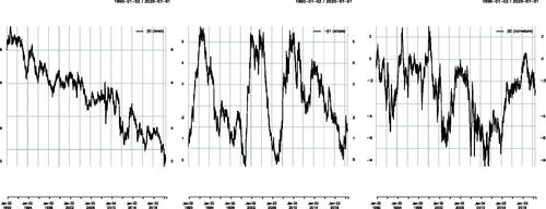
To estimate the yield curve, we proceed as follows. Following Diebold and Li (2006) we set the parameter τ in NS model equal to 1.37 = 1/(12 × 0.0609) at all dates, and choose the three remaining parameters that minimize the weighted sum of the absolute deviations between market prices of the US Treasuries and prices implied by the model. Following Gürkaynak, Sack, and Wright (2007), the weights chosen in the objective function are inversely proportional to the duration of each individual security. The reason is that the deviation between the actual and predicted prices of an individual security is approximately equal to its duration multiplied by the deviation between the actual and model implied yields. Thus, this procedure aims to minimize the (unweighted) sum of the absolute deviations between the actual and model implied yields on all of the securities. The resulting yield curve parameters are presented in Figure 1, which are then used to estimate the retirement bond price, its sensitivities relative to the three NS factors, as well as the sensitivities of the bonds used as hedging instruments.

Figure 1. Yield Curve’s Level (Left Panel), Slope (Middle) and Curvature (Right Panel) Nelson–Siegel Model Parameters Estimated from Bond Prices, Assuming a Fixed Shape Parameter Equal to $\tau$= 1.37 = 1/(12 × 0.0609) as in Diebold and Li (2006)

We consider a retirement bond with an initial time-to-maturity of 25 years, with a 5-year accumulation phase, during which no coupons are paid, and a 20-year decumulation period during which income is paid every month.¹⁵ Our sample period covers 25 years of historical data from July 3, 1995, to June 30, 2020.

To build the hedging portfolios, on each rebalancing date, we pick the bonds with over one month of remaining time-to-maturity to avoid having to drop bonds in between rebalancing dates. To remove redundant bonds, and try to avoid matrix singularity problems, we sort bonds by duration on each rebalancing date, then we round the duration figures to two digits and remove duplicates (i.e., we remove bonds with almost the same duration). All hedging strategies are rebalanced monthly.

Hedging Performance Measures

In this exercise, we aim to build a liability-hedging portfolio that replicates as closely as possible the value of the aforementioned retirement bond. To measure the quality of replication by a given hedging strategy, we first measure for each hedging strategy the time variations of its funding ratio, defined as the value of the cumulative total return of the replicating portfolio divided by the cumulative total return of the retirement bond portfolio to be replicated. Intuitively the funding ratio provides an estimate for the coverage level of the liability stream with the assets held in the portfolio. Setting both portfolios to have the same initial value, the initial funding ratio is equal to $100\%.$ A perfect replication would lead to a funding ratio staying constant at $100\%,$ and large changes in the funding ratio indicate the presence of large residual risk in hedging strategies. More generally, a change of $x\%$ in the funding ratio implies the same percentage change in terms of the affordable retirement income generated by the hedging portfolio relative to what would be affordable with perfect replication, i.e., with the retirement bond itself. We thus measure the out-of-sample quality of replication with the following indicators:

• FR.MEAD: median absolute deviation (with respect to 100%) of the daily funding ratio of the strategy, in percentage points, a measure of average risk.

• FR.MAAD: maximum absolute deviation (with respect to 100%) of the daily funding ratio of the strategy, in percentage points, a measure of extreme risk.

Besides measuring deviations in funding ratios, we also characterize the out-of-sample deviations in yield curve factor sensitivities of the hedging strategies relative to the sensitivities of the retirement bond. In particular, we report for all strategies the median and the maximum absolute deviations in the first- and second-order NS factor sensitivities with respect to the corresponding sensitivities for the retirement bond. Intuitively, the first-order sensitivity of a bond portfolio with respect to a given factor (say the slope of the yield curve) represents an estimate of the approximate (positive or negative) change in value of the bond portfolio following a small change in the corresponding factor (say a small steepening or flattening move). In the same spirit, the second-order sensitivity of a bond portfolio with respect to the slope of the yield curve represents an estimate of the approximate change in the first-order sensitivity value of the bond portfolio following a small steepening or flattening move. Incorporating second-order sensitivities in interest rate immunization strategies allows one to obtain a better hedging efficiency in case of a larger change in the value of underlying factors.

We divide the absolute deviations series by the median absolute value of the corresponding sensitivity of the retirement bond, to express them as percentages, thus controlling for differences in scale. In the tables, these median and maximum deviations in first-order factor exposures are denoted as Di.MEAD and Di.MAAD, respectively (for i = 0,1,2), when they apply to the ith factor in NS model. For the deviations in second-order exposures they are denoted DiDj.MEAD and DiDj.MAAD, respectively (for i,j = 0,1,2).

In addition, we report the median and maximum leverage of each strategy over the sample period (denoted Med Lev and Max Lev in the tables). The (gross) leverage of the portfolio $x$ on each date is calculated as in Equation (8)(8) $$L\left(x\right)≔\sum _{i=1}^n\left|x_i\right|$$(8) . We also report the average one-way monthly turnover (TO), and the average number of constituents (NC) of each hedging portfolio.

Out-of-Sample Performance of Hedging Strategies

For comparison purposes, first consider two simple single-factor strategies aiming at immunizing changes in portfolio values with respect to changes in the level of interest rates without regularization constraints.¹⁶ The first strategy only aims to match the duration of the retirement bond. This “Duration Barbell” strategy is implemented by selecting the bond with the longest duration available at each rebalancing date and the shortest duration bond (“cash”) to make the balance, and its weights are chosen to match the duration of the retirement bond Duration (hence H in Equation (5)(5) $$x^{\mathrm{*}}=H^{-1}D$$(5) is a 2 by 2 matrix in this case). The second strategy matches the Duration and Convexity of the retirement bond at each rebalancing date (see the exact-solution approach in Equation (5)(5) $$x^{\mathrm{*}}=H^{-1}D$$(5) ), which requires selecting three bonds. This Duration-Convexity strategy is implemented by selecting the bond with the longest duration, the bond with the median duration, and the bond with the shortest duration (“cash”) among the set available at each rebalancing date. Technically, the weights are calculated on each month end by Equation (5)(5) $$x^{\mathrm{*}}=H^{-1}D$$(5) , where H is a 3 by 3 matrix containing the Duration and Convexity of the three bonds (stacked with a vector of ones to ensure that the sum of weights equals 1), and the vector D contains the Duration and Convexity of the retirement bond, and the constant 1 (the sum of weights).

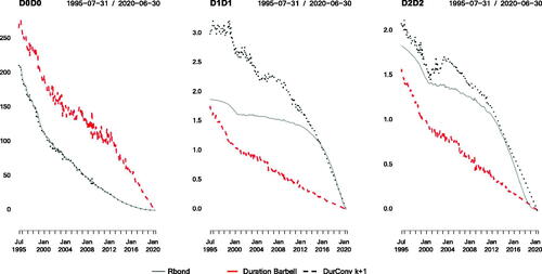
Figures 2 and 3 present the time series of the first- and second-order sensitivities to the NS factors of the retirement bond, and of the Duration Barbell and Duration-Convexity strategies. As expected, in the upper-right panel of Figure 2 we observe that these strategies do not exhibit significant deviations in terms of the first-order (FO) sensitivity to the level factor (denoted $D0=\frac{F_{{\beta }_0}}{F}$) at any point in time. Furthermore, in the left panel of Figure 3 we can see that the Duration-Convexity strategy does not present any noticeable deviations in the second-order (SO) sensitivity to the level factor (denoted D0D0), as expected. On the other hand, we observe that the Duration Barbell strategy does present a significant and persistent bias in its second-order sensitivity to the level factor. This can also be observed in Table 2, where we see that the median absolute deviation to the level factor, D0.MEAD, is equal to 1.9% for the Duration Barbell strategy, compared to 0.6% for the Duration-Convexity strategy. Moreover, the maximum absolute deviation in first-order sensitivities to the level factor, D0.MAAD, is 18% for the Duration Barbell strategy compared to 5.2% for the Duration-Convexity strategy.

Figure 2. Funding Ratio and First-Order Sensitivities to the NS Factors of the Retirement Bond (Continuous Line), the Duration Barbell (Dashed Line), and the Duration-Convexity (Dotted Line) strategies implemented with k + 1 Bonds, Where k Is the Number of Factor Sensitivities Matched by the Strategy (2 and 3 for the Duration and Duration-Convexity Strategies, Respectively)

The upper-left panel presents the time series of the funding ratios, the upper-right panel presents the first-order sensitivities to the level factor (D0), the bottom-left panel the first-order sensitivities to the slope factor (D1), and the bottom-right panel presents the first-order sensitivities to the curvature factor (D2).

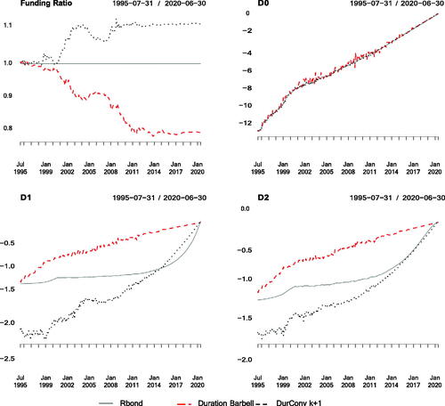
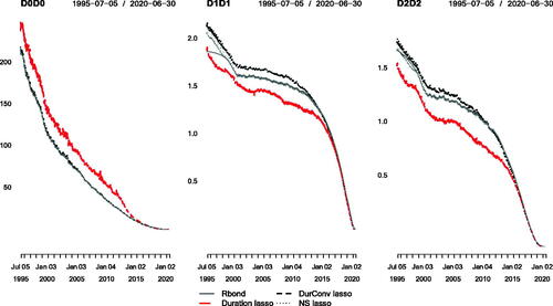
Figure 3. Second-Order Sensitivities to the NS Factors of the Retirement Bond (Continuous Line), the Duration Barbell (Dashed Line) and the Duration-Convexity (Dotted Line) Strategies Implemented with k + 1 Bonds, Where k Is the Number of Factor Sensitivities Matched by the Strategy (2 and 3 for the Duration and Duration-Convexity Strategies, Respectively)

The left panel presents the time series of the second-order sensitivities to the level factor (D0D0), the middle panel the second-order sensitivities to the slope factor (D1D1), and the bottom-right panel presents the first-order sensitivities to the curvature factor (D2D2).

The larger deviations in the second-order sensitivity to ${\beta }_0$ of the Duration Barbell strategy is expected to negatively impact the out-of-sample hedging performance of the strategy in case of large changes in the level of the yield curve between rebalancing dates. Our analysis confirms this intuition since it shows that the Duration-Convexity strategy, which exhibits lower bias in its second-order sensitivity to the level factor, presents a median and a maximum absolute deviation in funding ratio of 11.27% and 14.28%, while the Duration Barbell strategy exhibits a median and maximum deviation of 11.73% and 22.46%, respectively (see Table 1, panel A). The latter imply large levels of uncertainty in the purchasing power of the retirement assets in terms of retirement income.

Table 1. Number of Constituents (NC), Median and Maximum Leverage (Med Lev, Max Lev), Final Funding Ratio (FR.Final), Funding Ratio Median Absolute Deviation (FR.MEAD) and Maximum Absolute Deviation (FR.MAAD), and Average One-Way Monthly Turnover (TO) of Hedging Strategies Matching the Retirement Bond Yield Curve Factor Sensitivities Rebalanced Monthly

	NC	Med Lev	Max Lev	FR.Final	FR.MEAD	FR.MAAD	TO
A. Unrestricted leverage
Duration Barbell	2	1	1.13	78.93	11.73	22.46	68.1
DurConv k + 1	3	1.77	3.48	112.17	11.27	14.28	159.93
NS k + 1	4	31.44	6703.9	8.28	161.24	351.86	20737.88
B. Restricted leverage—L3
Duration lasso	127	1	1.32	96.21	2.05	3.80	8.58
DurConv lasso	87	1.02	1.64	102.04	2.37	3.77	12.6
NS lasso	83	1	1.53	100.75	1.74	3.39	17.89
C. Long-only
Duration lasso	127	1	1	95.25	1.48	4.76	9.16
DurConv lasso	84	1	1	101.06	1.54	2.90	10.67
NS lasso	82	1	1	99.46	0.61	2.92	16.27

Panel A corresponds to the strategies without regularization/leverage constraints. Panel B presents the regularized lasso strategies with a (gross) leverage limit of 3. Panel C presents the long-only lasso strategies.

The lower panels of Figure 2 also show that the Duration Barbell and Duration-Convexity strategies present large and persistent deviations in the first-order (FO) sensitivities to the slope and curvature factors (denoted by D1 and D2), as expected for single-factor immunization strategies that solely focus on changes in the level of interest rates. Indeed, in the first two columns of Table 2 we see that the (scaled) median absolute deviation and maximum absolute deviation in the FO sensitivity to the slope factor (D1.MEAD and D1.MAAD) of the Duration Barbell strategy are 47.0% and 71.1%, respectively, and the corresponding numbers for the Duration-Convexity are 38.8% and 102.4%. Moreover, the median and maximum absolute deviations in the FO sensitivity to the curvature factor (D2.MEAD and D2.MAAD) of the Duration Barbell strategy are 46.1% and 66%, respectively, and 32.9% and 70.1% for the Duration-Convexity strategy. Furthermore, Figure 3 shows that both strategies also present important biases in the second-order sensitivities relative to the slope, and curvature factors, D1D1 and D2D2. Besides, from Figures 2 and 3, note that the biases in all factor sensitivities of the Duration Barbell and Duration-Convexity strategies have opposite signs during most of the sample, and their deviations in terms of funding ratio from the retirement bond, observed in the upper-left panel of Figure 2, also have opposite signs.

Table 2. Summary of Deviations in NS Factor Sensitivities of Hedging Strategies Relative to the Retirement Bond

	Duration Barbell	DurConv k + 1	NS k + 1	Duration lasso	DurConv lasso	NS lasso
D0.MEAD	0.019	0.006	0.018	0.006	0.006	0.007
D0.MAAD	0.180	0.052	3,646.864	0.055	0.051	0.087
D1.MEAD	0.470	0.388	0.009	0.051	0.041	0.009
D1.MAAD	0.711	1.024	1,635.570	0.092	0.224	0.168
D2.MEAD	0.461	0.329	0.008	0.106	0.042	0.008
D2.MAAD	0.660	0.701	1,703.917	0.166	0.163	0.110
D0D0.MEAD	1.471	0.013	1.426	0.408	0.007	0.004
D0D0.MAAD	2.159	0.180	12,129.316	0.873	0.117	0.138
D1D1.MEAD	0.477	0.412	0.013	0.083	0.049	0.008
D1D1.MAAD	0.701	0.945	1,747.534	0.139	0.203	0.145
D2D2.MEAD	0.431	0.123	0.045	0.151	0.026	0.007
D2D2.MAAD	0.624	0.279	1,614.618	0.214	0.088	0.046
D0D1.MEAD	0.029	0.028	0.018	0.010	0.006	0.006
D0D1.MAAD	0.164	0.144	3,715.280	0.054	0.035	0.074
D0D2.MEAD	0.043	0.108	0.031	0.014	0.009	0.006
D0D2.MAAD	0.218	0.359	3,805.218	0.065	0.058	0.056
D1D2.MEAD	0.451	0.287	0.009	0.124	0.039	0.007
D1D2.MAAD	0.649	0.559	1,678.741	0.187	0.137	0.087

MEAD stands for median absolute deviation and MAAD for maximum absolute deviation. For instance, D0.MEAD stands for median absolute deviation in sensitivity to ${\beta }_0$ (the level factor) between each strategy and the corresponding sensitivity of the retirement bond over time. D1.MAAD is the maximum absolute deviation in first-order sensitivity with respect to ${\beta }_1$ (slope) from the sensitivity of the retirement bond, and D1D1.MAAD is the maximum absolute deviation in the second-order sensitivity with respect to ${\beta }_1.$ All MEAD and MAAD series are divided by the median value of the corresponding retirement bond’s factor sensitivity, to express them as percentages.

The key insight in this analysis is that these single-factor immunization strategies can imply very significant levels of unintended biases in the first- and second-order sensitivities to the slope and curvature factors, as expected since the exposure to these factors are not controlled for by the Duration and Convexity strategies. In contrast, we confirm that a multifactor “NS k + 1” strategy presents relatively low biases in the first-order sensitivities to the three NS factors. As Table 2 shows, the median absolute deviations in its FO sensitivity to the level factors (D0.MEAD) is 1.8% (slightly lower than the respective figure of 1.9% for the Duration Barbell strategy), and the median absolute deviations in its FO sensitivities to the slope and curvature factors are 0.9% and 0.8%, which are significantly lower than the corresponding figures for the Duration Barbell and Duration-Convexity strategies (see the D1.MEAD and D2.MEAD in Table 2 for these two strategies, which are 47%, 38.8%, and 46.1%, 32.9%, respectively).

These results suggest that strategies aiming to match factor exposures beyond the level factor could a priori improve hedging performance. However, we also find that using the exact-solution approach (see Equation 5(5) $$x^{\mathrm{*}}=H^{-1}D$$(5) ) to match the FO sensitivities to the three NS factors results in a strategy with an extreme leverage level (see panel A of Table 1). Indeed, the strategy is found to exhibit extremely large deviations from its well-aimed median sensitivities, as reflected in its maximum deviations relative to all the NS factor exposures. Indeed, all the MAAD figures in Table 2 that correspond to the NS k + 1 strategy, are above 161,461, contrasting with the corresponding figures of the other strategies. The extreme variability in its factor exposures is caused by the extreme weights and leverage that results for this strategy using the exact-solution approach. This large instability in factor exposures results in very poor hedging performance (see the NS k + 1 row in Table 1).

To address the conundrum of having either uncontrolled biases in slope and curvature factors exposures, as with Duration and Duration-Convexity strategies, or the extreme instability in factor exposures of the NS k + 1 strategy, we now analyze the performance of a regularization approach (that we call the lasso strategies) which minimize the squared deviations in first- and second-order NS factor exposures under leverage constraints. As observed in Table 2, panel B, the NS lasso strategy implemented with a maximum gross leverage limit ($\overline{\delta }$) of 3, presents lower median and maximum absolute deviations in all NS factor sensitivities than the Duration Barbell strategy and in 16 out of the 18 MEAD and MAAD metrics compared to the Duration-Convexity strategy. The enhanced control in factor exposures implied by leverage constraints translates into an economically significant improvement in hedging performance. As observed in Table 1, the maximum absolute deviations in funding ratio for the Duration Barbell and Duration-Convexity strategies are 22.46% and 14.28%, respectively, while it is only 3.39% for the NS lasso strategy. This represents a remarkable low level of risk, leaving investors with a funding ratio that stays in a narrow (96.61%–103.39%) range. In practice, the improvement in hedging performance net of transaction costs would actually be higher given that the average monthly turnover of the NS lasso strategy is almost four times lower than the turnover of the Duration Barbell strategy, and almost nine times lower than the turnover of the Duration-Convexity strategy.¹⁷

We also simulate the NS lasso strategy with a limit on gross leverage ($\overline{\delta }$) of 1, effectively corresponding to a long-only constraint. Comparing panels B and C of Table 1, we can observe that tightening the leverage constraint to its maximum, produced some slight improvement in hedging performance for the strategy. The maximum absolute deviation in funding ratio decreases from 3.39% to 2.92%. These results are in stark contrast with the corresponding numbers obtained for the Duration and Duration-Convexity, of 22.46% and 14.28%. The conclusion from this analysis is that limiting leverage to a reasonable and controlled level in NS factor immunization strategies can induce large improvements in out-of-sample hedging performance. Interestingly, the NS lasso strategy under the leverage limit of 3 does not use all the available leverage budget, since it exhibits a maximum leverage over the period of only 1.53, a number higher than 1 but much lower than the maximum leverage level of 3.48 obtained with the unrestricted Duration-Convexity strategy (see Max Lev column in panel A of Table 1).

Regularized Duration and Convexity Hedging

To assess the marginal improvement generated by hedging slope and curvature factors, we next consider a regularized version of the single-factor hedging strategies, namely, the Duration-Matching and Duration-Convexity matching strategies. The goal here is to minimize the squared difference between the duration (or duration and convexity) of the hedging portfolio and the retirement bond liability to be replicated, under the constraints of keeping the gross portfolio leverage under 3, and shorting allowed only in “cash”. One key difference between these regularized strategies and the duration strategy (respectively, duration and convexity) tested before, is that the latter requires the selection of a basket of two bonds (respectively, three bonds) to avoid an over-specified problem. On the other hand, in the regularized optimization setting, the strategy can potentially allocate to all the bonds available. As can be observed in Table 2, this so-called Duration lasso strategy presents lower median and maximum absolute deviations in all NS factor sensitivities than the unconstrained Duration Barbell strategy. This reduction in bias and variance of factor exposures is expected to reflect in lower replication error. Indeed, the maximum absolute deviation in funding ratio of the Duration lasso strategy is 3.80% compared to 22.46% for the Duration Barbell strategy (see panels A and B of Table 1), which represents a reduction of almost 6 times the uncertainty around the level of retirement income secured with the bond portfolio. In practice, this improvement in hedging performance would be higher because the strategy involves a remarkable reduction in turnover. The average monthly turnover of the Duration lasso strategy is 8.58% compared to 68.1% for the Duration Barbell strategy.

A similar improvement is observed when comparing the Duration-Convexity lasso strategy (with $\overline{\delta }$=3) with the unrestricted Duration-Convexity strategy. The regularized strategy presents a median and maximum absolute deviation in funding ratio of 2.37% and 3.77%, compared to 11.27% and 14.28% for the unrestricted Duration-Convexity strategy. Furthermore, the Duration-Convexity lasso strategy generates an average turnover of 12.6% compared to 159.93% for the unrestricted strategy. The notable improvement in hedging performance can be explained by the significant decrease in the median and maximum deviations in exposures to the slope and curvature factors. For instance, the median absolute deviation in exposures to the slope and curvature factors for the unrestricted Duration-Convexity strategy are 38.8% and 32.9%, compared to 4.1% and 4.2% for the Duration-Convexity lasso strategy (see Table 2, columns DurConv k + 1 and DurConv lasso, rows D1.MEAD and D2.MEAD). More generally, this regularized strategy presents lower values in all the MEAD and MAAD factor exposure metrics, compared to the unrestricted Duration-Convexity strategy.

It is interesting to notice that the regularized Duration lasso and Duration-Convexity lasso strategies implemented with leverage constraints allow for such a significant improvement in terms of their deviations in factor exposures to the slope and curvature factors, even though they do not explicitly aim to minimize these deviations in their design. Given that the lasso strategies are not restricted to use a subset of the bonds available, they are much less conditioned by the individual characteristics (i.e., yield factor exposures) of the constituent bonds than the unrestricted exact-solution version of the strategy, which leads to enhanced robustness. However, we expect that explicitly targeting factor exposure matching for all 3 factors, as done with the NS lasso strategy, should lead to improved hedging performance. To analyze this, we report in Figures 4 and 5 the time series of first- and second-order sensitivities of the three lasso strategies matching Duration, Duration-Convexity and the NS factor sensitivities. Indeed, the latter strategy presents factor sensitivities that are consistently closer to the ones of the retirement bond liability. Moreover, as observed in Table 2, the NS lasso strategy presents lower values in 13 and 14 out of the 18 MEAD and MAAD metrics compared to the Duration lasso and Duration-Convexity lasso strategies. As expected, this better matching of factor exposures results in an improvement in terms of hedging performance. Indeed, the maximum absolute deviations of the funding ratio for Duration lasso and Duration-Convexity lasso strategies, with a value reaching 3.80% and 3.77%, respectively, are higher than the corresponding measure for the NS lasso strategy at 3.39%, and this for the same leverage limit of 3. Moreover, the median absolute deviations in funding ratio of the Duration lasso and Duration-Convexity lasso strategies, reaching, respectively, 2.05% and 2.37%, is also higher in an economic sense, than the 1.74% value obtained with the NS lasso strategy (see panel B in Table 2).

Figure 4. Funding Ratio and First-Order Sensitivities to the NS Factors of the Retirement Bond (Continuous Line), and the Hedging Strategies Implemented with All the Bonds Available and with a Lasso Regularization that Restricts the Gross Leverage below Three at All Times

Strategies matching Duration, Duration and Convexity, and the strategy matching the first- and second-order sensitivities to the three NS factors. The upper-left panel presents the time series of the funding ratios, the upper-right panel presents the first-order sensitivities to the level factor (D0), the bottom-left panel the first-order sensitivities to the slope factor (D1), and the bottom-right panel presents the first-order sensitivities to the curvature factor (D2).

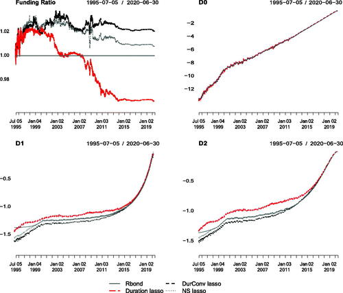
Figure 5. Second-Order Sensitivities to the Three NS Factors of the Retirement Bond, and of the Hedging Strategies Implemented with All the Bonds Available and with a Lasso Regularization that Restricts the Gross Leverage below Three at All Times

Strategies matching Duration, Duration and Convexity, and the strategy matching the first- and second-order sensitivities to the three NS factors. The left panel presents the time series of the second-order sensitivities to the level factor (D0D0), the middle panel the second-order sensitivities to the slope factor (D1D1), and the right panel presents the second-order sensitivities to the curvature factor (D2D2).

Panel C of Table 1 presents the performance summary for the Duration lasso and Duration-Convexity lasso strategies implemented with the long-only constraint ($\overline{\delta }$=1). In comparison with the long-only NS lasso strategy, we observe a similar pattern, that is, we find that the latter strategy presents an economically meaningful improvement in hedging performance relative to the strategies that only take into account Duration or Duration and Convexity under the same regularized framework. Indeed, the long-only NS lasso presents a FR.MEAD of 0.61% compared to 1.54% and 1.48% for the long-only Duration-Convexity lasso and Duration lasso strategies, respectively. This improvement in hedging performance is also consistent with the lower deviations in factor exposures. We report in Table 3 the median and maximum absolute deviations in the factor sensitives of the lasso strategies matching Duration, Duration-Convexity and NS factors implemented with the long-only constraint ($\overline{\delta }$=1). We find that the long-only NS lasso strategy presents lower or equal values in 14 out of the 18 MEAD and MAAD measurements than the Duration lasso and Duration-Convexity lasso strategies, respectively.

Table 3. Summary of Deviations in NS Factor Sensitivities of Long-Only Hedging Strategies Relative to the Retirement Bond

	Duration Lasso	DurConv Lasso	NS Lasso
D0.MEAD	0.006	0.006	0.007
D0.MAAD	0.165	0.283	0.289
D1.MEAD	0.054	0.027	0.010
D1.MAAD	0.107	0.099	0.099
D2.MEAD	0.111	0.033	0.008
D2.MAAD	0.207	0.201	0.201
D0D0.MEAD	0.408	0.007	0.005
D0D0.MAAD	1.406	0.120	0.104
D1D1.MEAD	0.087	0.034	0.009
D1D1.MAAD	0.159	0.154	0.154
D2D2.MEAD	0.153	0.027	0.007
D2D2.MAAD	0.296	0.291	0.291
D0D1.MEAD	0.010	0.007	0.007
D0D1.MAAD	0.185	0.308	0.313
D0D2.MEAD	0.014	0.010	0.007
D0D2.MAAD	0.218	0.348	0.354
D1D2.MEAD	0.128	0.035	0.008
D1D2.MAAD	0.239	0.233	0.233

MEAD stands for median absolute deviation and MAAD for maximum absolute deviation. Hence, for instance, D0.MEAD stands for median absolute deviation in sensitivity to ${\beta }_0$ (the level factor) between each strategy and the corresponding sensitivity of the retirement bond over time. D1.MAAD is the maximum absolute deviation in first-order sensitivity with respect to ${\beta }_1$ (slope) from the sensitivity of the retirement bond, and D1D1.MAAD is the maximum absolute deviation in the second-order sensitivity with respect to ${\beta }_1.$ All MEAD and MAAD series are divided by the median value of the corresponding retirement bond’s factor sensitivity, to express them as percentages.

Comparing the corresponding columns in Tables 2 and 3, we note that the Duration lasso strategy implemented with a leverage limit of 3 has lower values in all of the MEAD and MAAD factor exposure deviations compared to the corresponding Duration lasso strategy implemented with zero tolerance for leverage (i.e., $\overline{\delta }$=1). This suggests that a reasonable degree of leverage, if limited and controlled, is expected to improve hedging performance.

Finally, we have also simulated strategies minimizing the squared deviations in the first- and second-order sensitivities of the NS bond price with respect to time. These results suggest that matching the time sensitivities has a negligible effect on the hedging performance of the lasso strategy that takes into account the three NS factors. This is presumably because matching the exposure to a relatively exhaustive set of risk factors implies by the absence of arbitrage a reasonably good matching of expected return components. On the other hand, we find that adding the minimization of deviations in the time sensitivities to strategies matching only Duration or Duration-Convexity with the lasso approach significantly decreases deviations in slope and curvature sensitivities and improves the hedging performance to an economically meaningful extent.¹⁸

Conclusion

Hedging against non-parallel shifts in the yield curve is of major practical importance for institutions like pension funds or insurance companies endowed with long-term liabilities. Indeed, the fair value of a long-term stream of liability cash flows, such as promised pension payments for the beneficiaries of a defined-benefit pension fund, can be obtained as the discounted value of the cash flows. Thus being a complex function of the whole yield curve, an infinite-dimensional risk factor. Fortunately, it has been shown that three main factors, namely, the level, slope, and curvature of the yield curve, explain a large fraction of the changes in the term structure of interest rates. In this context, efficient immunization strategies can be obtained in principle by holding liability-hedging bond portfolios matching at every trading date the exposure of the stream of liability cash flows with respect to changes in these three risk factors to the first and possibly second-order.

In implementation, however, the weights of these hedging portfolios obtained as unconstrained solutions to the yield curve multifactor exposure matching problem, results in extremely large portfolio weights. The latter implies exceedingly high levels of leverage, turnover, and unstable factor exposures between portfolio rebalancing dates.

This paper proposes to address this issue with regularization procedures in the factor exposure matching problem, based on the introduction of a lasso penalty and leverage constraints. These procedures, borrowed from the machine learning literature, have proven effective in addressing the lack of robustness of mean-variance portfolio optimization in equity markets, and this paper shows that they are also helpful in the construction of interest rate hedging strategies. In out-of-sample empirical backtests, we confirm that these generalized immunization strategies offer both a substantial improvement in hedging performance and a strong reduction in leverage and turnover compared to an unconstrained approach to bond portfolio immunization.

Acknowledgements

Daniel acknowledges financial support from Universidad de los Andes (grant number P18.100322.008).

Disclosure Statement

No potential conflict of interest was reported by the author(s).

Additional information

Funding

Daniel acknowledges financial support from Universidad de los Andes (grant number P18.100322.008).

Notes on contributors

Daniel Mantilla-Garcia

Daniel Mantilla-Garcia is an Assistant Professor at Universidad de Los Andes, School of Management.

Lionel Martellini

Lionel Martellini is a Professor of Finance at EDHEC Business School, Nice, France.

Vincent Milhau

Vincent Milhau is a Research Director of EDHEC-Risk Institute, Nice, France.

Hector Enrique Ramirez-Garrido

Hector Enrique Ramirez-Garrido is a Research Assistant at Universidad de Los Andes, School of Management.

Notes

1 Furthermore, Redington (1952) determined the conditions under which Duration-matching of multiple cash flows results in local immunization, while Bierwag, Kaufman, and Toevs (1983) established the conditions under which Duration-matching implies global immunization in presence of level shifts, and Barber (1999) generalized these results to the single-factor affine term structure model.

2 We show that the unconstrained multifactor approach produces extreme weights even if the input parameters, e.g., yield curve’s level, slope and curvature in the Nelson and Siegel (1987) model, present stable dynamics reflecting their economic interpretation.

3 However, F is still right differentiable with respect to time on these dates.

4 By Schwarz’s theorem, the cross derivatives $F_{ij}$ and $F_{ji}$ are equal for any two indices i and j.

5 See Appendix A for a formal discussion of this argument.

6 This unique and exact-solution hedging approach in Equation (5)(5) $$x^{\mathrm{*}}=H^{-1}D$$(5) appears for instance in text books such as Fabozzi, Martellini, and Priaulet (2005) and Martellini, Priaulet, and Priaulet (2003). When there are more constituent bonds than constraints, the linear system (4) is underdetermined.

7 A portfolio with extremely large weights has factor exposures that are very sensitive to small changes in the factor exposures of the constituents. To illustrate this effect, we have simulated a strategy matching the first-order sensitivities to the three factors rebalanced every day, and it turns out to have large deviations in second-order sensitivities and poor out-of-sample hedging performance. These results are unreported for the sake of brevity but are available upon request from the authors. Moreover, the strategy aiming to match first- and second-order sensitivities to the NS factors with the exact solution in Equation (5)(5) $$x^{\mathrm{*}}=H^{-1}D$$(5) , was not feasible as the matrix H was ill-conditioned and numerically not invertible.

8 If $n\ge k+1,$ the rank of $H$ is at most $k+1.$ Therefore, $H\prime H,$ which is a $n\times n$ matrix, is singular except if $n=k+1,$ because $H\prime H$ and $H$ have the same rank. Note Equation (7)(7) $$x^{\mathrm{*}}={\left(H\mathrm{\prime }H\right)}^{-1}\left(H\mathrm{\prime }D\right)$$(7) has the same functional form as the OLS estimator in a multivariate regression. Note as well that in the particular case in which the number of bonds available is equal to k + 1, then H is a squared matrix and the weight vector $x^{*}$ simplifies to the exact-unique solution strategy in Equation (5)(5) $$x^{\mathrm{*}}=H^{-1}D$$(5) . Hence, the exact-solution approach to multifactor immunization (Equation (5)(5) $$x^{\mathrm{*}}=H^{-1}D$$(5) ) is a special case of this generalized approach, as the latter reduces to the exact-solution immunization strategies if (i) the hedging portfolio is constrained to use only a small subset of the available hedging instruments so that the number of portfolio constituents equals the number of factor exposures to match, n = k + 1, and if (ii) the forecasts of factor exposures are assumed to have zero error (in which case, no regularization constraints would be needed).

9 Since the matrix $\mathrm{\Lambda }=H\prime H$ in Equation (9)(9) $$\underset{x}{\min }\frac{x^{\mathrm{\prime }}\mathrm{\Lambda }\mathrm{x}}{2}-{\mathrm{x}}^{\mathrm{\prime }}\mathrm{\Theta }+\mathrm{\lambda }\left(\sum _{i=1}^n\left|x_i\right|\right)$$(9) is singular, in order to use a faster standard quadratic programming optimizer, we add a small perturbance term (0.00001) to its diagonal, which is equivalent to a ridge regularization.

10 We also consider the ridge and lasso strategies without the restriction to limit short positions to cash. In our empirical simulations of these strategies, we observe that for the strategy hedging only the first-order sensitivities to the three NS factors, this additional restriction did have some negative effect on hedging performance. However, for the strategies hedging up to the second-order sensitivities to the NS factors, that additional restriction did not have a negative impact on hedging performance. These results are available from the authors upon request.

11 If the number of bonds, n, is greater than the number of linear constraints, i.e., k + 1, the system in $Hx=D$ has infinitely many solutions, all of which are factor-matching portfolios. Some of those solutions have more extreme weights, and hence more unstable factor exposures. Another alternative to regularize the strategy is selecting the portfolio that minimizes the weights’ squared second norm, subject to the linear constraints $Hx=D.$ The main problem that we saw with that approach, is that the constraint to have an exact match of the target factor exposures can be too restrictive, in the sense that it can result in solutions in which the weights are still too large, hence still leading to high factor exposure instability of the hedging portfolio. Indeed, in our empirical tests of this norm minimization strategy, the maximum leverage presented over the simulation was above 4, which might be too high in some contexts, and beyond the leverage limit of 3 that we considered. The results for the ridge strategy and the norm minimization are unreported for the sake of brevity, but available upon request from the authors.

12 Life expectancy at age 65 for a generic US individual was 19.5 years in 2018 (see Table B in National Vital Statistics Reports 2021: Arias, Brigham, and Tejada-Vera 2021). Note that the retirement bonds replicated in this exercise do not address longevity risk beyond life expectancy.

13 To obtain protection against unexpected inflation risk, one would need an inflation-linked retirement bond, which could be priced using the real, as opposed to nominal, zero-coupon yield curve, implying that the hedging instruments would be inflation-protected bonds.

14 The data extraction process is as follows: using the SRCH command in the Bloomberg terminal, we obtain the full bonds’ ID list (for both corporate and public debt). Then, we restrict the “Asset Classes” query to “Government bonds”, and for “Security Status” we allow “Active and Matured securities”, set the “Issuer” column to “United States”, and fix the “Maturity Type” as “Normal” (excluding for instance callable bonds). Then, we filter to use only “T” bond series, i.e., Treasury bonds, thus excluding SP, SPX, SPY series (i.e., Strip Principal bonds).

15 We aim to replicate a retirement bond with 25 years of initial time-to-maturity as Bierwag, Kaufman, and Toevs’s (1983) immunization theorem suggests that the range of dates of cash flow for the liability stream should be within the range of available durations for the hedging instruments.

16 These strategies are special cases of the exact-solution approach in Equation (5)(5) $$x^{\mathrm{*}}=H^{-1}D$$(5) .

17 This large improvement in turnover is partly related to the fact that the NS lasso strategy does not need to use a new selection of k+1 bonds at each rebalancing date but uses all bonds available.

18 The results of the strategies matching time derivatives are unreported for the sake of brevity but are available upon request from the authors.

19 Note that because second-order derivatives are symmetric in the indices p and q, it suffices to consider only pairs for which p≤q.

Appendix A. Bond Factor Exposures in Nelson–Siegel Model

 

If the excess return of the portfolio over the bond is perfectly immunized against changes in factor values, it must be the case that the portfolio exposures match those of the target replicated bond. So, we have, for p ranging from 0 to 3, $$\sum _{i=1}^N{w}_{it}\frac{F_p^{\left(i\right)}}{F^{\left(i\right)}}=\frac{F_p}{F}.$$

In other words, a necessary condition for replication is that the portfolio exposure to each factor, defined as the weighted sum of the constituents’ exposures, match the target bond exposure. The previous calculation can be repeated with the second-order Taylor expansion of Equation (3)(3) $$r_{t,t+h}\approx \frac{F_0}{F}\Delta {\beta }_{0t}+\frac{F_1}{F}\Delta {\beta }_{1t}+\frac{F_2}{F}\Delta {\beta }_{2t}+\frac{F_3}{F}h+\frac{1}{2}\sum _{i,j=0}^3\frac{F_{ij}}{F}\Delta {\beta }_{it}\Delta {\beta }_{jt}.$$(3) , to show that the matching of second-order exposures is another necessary condition for replication. Mathematically, for any two indices p and q ranging from 0 to 3, we must have¹⁹ $$\sum _{i=1}^N{w}_{it}\frac{F_{pq}^{\left(i\right)}}{F^{\left(i\right)}}=\frac{F_{pq}}{F}.$$

The first-order exposures of the coupon-paying bond to the level, slope, and curvature factors are given by $$\frac{F_0}{F}=-\frac{1}{F}\sum _{s>t}C{F}_s{e}^{-\left[t_j-t\right]y_{t,s-t}}\left[s-t\right],$$ $$\frac{F_1}{F}=-\frac{1}{F}\sum _{s>t}C{F}_s{e}^{-\left[s-t\right]y_{t,s-t}}\left[s-t\right]f\left(\frac{s-t}{\tau }\right),$$ $$\frac{F_2}{F}=-\frac{1}{F}\sum _{s>t}C{F}_s{e}^{-\left[s-t\right]y_{t,s-t}}\left[s-t\right]g\left(\frac{s-t}{\tau }\right).$$

The pricing function is differentiable with respect to time before the first payment date. The right derivative is given by $$F_t=\sum _{s>t}C{F}_s{e}^{-\left[s-t\right]y_{t,s-t}}\left[y_{t,s-t}-\left[s-t\right]\frac{\partial y_{t,s-t}}{\partial t}\right],$$ where the time derivative of the zero-coupon yield is $$\frac{\partial y_{t,s-t}}{\partial t}=-\frac{1}{\tau }{f}^{\mathrm{\prime }}\left(\frac{s-t}{\tau }\right){\beta }_{1t}-\frac{1}{\tau }{g}^{\mathrm{\prime }}\left(\frac{s-t}{\tau }\right){\beta }_{2t}.$$

The second-order exposures with respect to the risk factors are given by $$\frac{F_{00}}{F}=\frac{1}{F}\sum _{s>t}C{F}_s{e}^{-\left[s-t\right]y_{t,s-t}}{\left[s-t\right]}^2,$$ $$\frac{F_{11}}{F}=\frac{1}{F}\sum _{s>t}C{F}_s{e}^{-\left[s-t\right]y_{t,s-t}}{\left[s-t\right]}^2{f\left(\frac{s-t}{\tau }\right)}^2,$$ $$\frac{F_{22}}{F}=\frac{1}{F}\sum _{s>t}C{F}_s{e}^{-\left[s-t\right]y_{t,s-t}}{\left[s-t\right]}^2{g\left(\frac{s-t}{\tau }\right)}^2,$$ $$\frac{F_{01}}{F}=\frac{1}{F}\sum _{s>t}C{F}_s{e}^{-\left[s-t\right]y_{t,s-t}}{\left[s-t\right]}^{2}f\left(\frac{s-t}{\tau }\right),$$ $$\frac{F_{02}}{F}=\frac{1}{F}\sum _{s>t}C{F}_s{e}^{-\left[s-t\right]y_{t,s-t}}{\left[s-t\right]}^{2}g\left(\frac{s-t}{\tau }\right),$$ $$\frac{F_{12}}{F}=\frac{1}{F}\sum _{s>t}C{F}_s{e}^{-\left[s-t\right]y_{t,s-t}}{\left[s-t\right]}^{2}f\left(\frac{s-t}{\tau }\right)g\left(\frac{s-t}{\tau }\right).$$

Appendix B. Implementation Details of Lasso Optimization

 

The optimization problem in Equation (9)(9) $$\underset{x}{\min }\frac{x^{\mathrm{\prime }}\mathrm{\Lambda }\mathrm{x}}{2}-{\mathrm{x}}^{\mathrm{\prime }}\mathrm{\Theta }+\mathrm{\lambda }\left(\sum _{i=1}^n\left|x_i\right|\right)$$(9) is equivalent to minimizing deviations in factor sensitivities subject to a leverage upper bound constraint: (B1) $${\displaystyle \underset{x}{\text{min}}}\frac{x^{\prime }\mathrm{\Lambda }x}{2}-x^{\prime }\mathrm{\Theta }.$$(B1) $$u.c.\mathrm{ }\{\begin{array}{c}{1}^{\mathrm{\prime }}x=1\\ \sum _{i=1}^n\left|x_i\right|\le \overline{\delta }\end{array}$$

For numerical efficiency reasons, rewrite the program (B1) by replacing the non-linear inequality constraint (the leverage constraint) with a set of linear constraints. To do so, define auxiliary variables denoted $x^{+}$ and $x^{-},$ such that $$x_i=\underset{i}{\overset{+}{x}}-\underset{i}{\overset{-}{x}}\mathrm{ }\forall i\in \{1,\dots n\}$$ with $x_i^{+}\ge 0$ and $x_i^{-}\ge 0.$ The leverage is then given by ${\sum }_{i=1}^n\left|x_i\right|={\sum }_{i=1}^n{x}_i^{+}+{\sum }_{i=1}^n{x}_i^{-},$ and we rewrite program (B1) as: $$\underset{x}{\min }\frac{x^{\prime }\mathrm{\Lambda }x}{2}-x^{\prime }\mathrm{\Theta }$$ $$\mathrm{u}.\mathrm{c}\mathrm{ }\{\begin{array}{c}{1}^{\mathrm{\prime }}x=1\\ x_i=x_i^{+}-x_i^{-}\\ \sum _{i=1}^n{x}_i^{+}+\sum _{i=1}^n{x}_i^{-}\le \overline{\delta }\\ x_i^{+}\ge 0;x_i^{-}\ge 0 \end{array}$$

Furthermore, this $n$-dimensional optimization problem is equivalent to the following standard quadratic programing (QP) problem of dimension of $3n$ with linear constraints: $$\underset{X}{\min }\frac{X^{\prime }GX}{2}-X^{\prime }R$$ $$\mathrm{u}.\mathrm{c}\mathrm{ }\{\begin{array}{c}AX=B\\ CX\ge F\end{array}$$ where $X={\left(x_1,x_2,\dots ,x_n,x_1^{+},x_2^{+},\dots ,x_n^{+},x_1^{-},x_2^{-},\dots ,x_n^{-}\right)}^{\prime },$ and $$G=\left(\begin{array}{ccc}\mathrm{\Lambda }& 0& 0\\ 0& 0& 0\\ 0& 0& 0\end{array}\right), R=\left(\begin{array}{c}\mathrm{\Theta }\\ 0\\ 0\end{array}\right), C=\left(\begin{array}{ccc}0& -1^T& -1^T\\ & I_{3n}& \end{array}\right),F=\left(\begin{array}{c}\begin{array}{c}-\overline{\delta }\\ -\infty \end{array}\\ 0_{3n-1}\end{array}\right)$$ $$A=\left(\begin{array}{ccc}{1}^T& 0& 0\\ I_n& I_n& -I_n\end{array}\right),\mathrm{\text{and}} B=\left(\begin{array}{c}1\\ 0\end{array}\right)$$

Note matrix F includes the constraints that all but the weight of the shortest maturity bond (i.e., cash) be positive. The matrix $G$ is not positive definite, which can be a problem to use some QP optimizers that assume a matrix with positive eigenvalues. Adding a small disturbance term (0.00001) do its diagonal eliminates the singularity problem. This is equivalent to a ridge regularization. We refer to the resulting portfolio $x^{\star },$ which is made of the first $n$ elements of the resulting $X^{\star },$ as the lasso strategy in the paper.

Appendix C. Ridge Strategy and the Leverage Constraint

 

Consider a variation of the program Equation (6)(6) $$\underset{x}{\min }\frac{1}{2}{x}^{\mathrm{\prime }}{H}^{\mathrm{\prime }}Hx-x^{\mathrm{\prime }}{H}^{\mathrm{\prime }}D$$(6) , with penalization for the output vector ${\mathcal{\ell }}_2$-norm: (C1) $$x^{\star }\left(\rho \right)=\arg \underset{x}{\min }\frac{x\mathrm{\prime }\mathrm{\Lambda }x}{2}-x\mathrm{\prime }\mathrm{\Theta }+\frac{\rho }{2}\left|\right|x|{|}_2^2\mathrm{u}.\mathrm{c}\mathrm{ }1\mathrm{\prime }x=1$$(C1) where $\left|\right|x|{|}_2^2={\sum }_{i=1}^n{x}_i^2$ is the squared ${\mathcal{\ell }}_2$-norm of $x.$ Recall the relationship between the Manhattan norm (leverage) and the ${\mathcal{\ell }}_2$-norm: $$\sum _{i=1}^n\left|x_i\right|=\left|\right|x|{|}_1\le \sqrt{n}\mathrm{ }{\left|\right|x\left|\right|}_2$$

Hence, a larger penalization parameter $\rho$ on the squared ${\mathcal{\ell }}_2$-norm in Equation (C1)(C1) $$x^{\star }\left(\rho \right)=\arg \underset{x}{\min }\frac{x\mathrm{\prime }\mathrm{\Lambda }x}{2}-x\mathrm{\prime }\mathrm{\Theta }+\frac{\rho }{2}\left|\right|x|{|}_2^2\mathrm{u}.\mathrm{c}\mathrm{ }1\mathrm{\prime }x=1$$(C1) implies a more strict leverage restriction on $x^{\star }(\rho ).$ In order to further characterize the ridge strategy, we solve analytically for $x^{\star }.$ The Lagrangian of problem (C1) reads $$\mathcal{L}(x,\lambda )=\frac{x^{\mathrm{\prime }}\mathrm{\Lambda }x}{2}-x^{\mathrm{\prime }}\mathrm{\Theta }+\frac{\rho }{2}{x}^{\mathrm{\prime }}{I}_{n}x-\lambda (1^{\mathrm{\prime }}x-1)$$

The first-order optimality conditions are $$x^{\star }=(\mathrm{\Lambda }+\rho I_n{)}^{-1}(\mathrm{\Theta }+{\lambda }^{\star }1)$$ $$1^{\mathrm{\prime }}x=1$$

Solving for ${\lambda }^{\star },$ we obtain $${\lambda }^{\star }=\frac{1-1^{\mathrm{\prime }}(\mathrm{\Lambda }+\rho I_n{)}^{-1}\mathrm{\Theta }}{1^{\mathrm{\prime }}(\mathrm{\Lambda }+\rho I_n{)}^{-1}1}$$ and the optimal ridge portfolio is (C2) $$x^{\star }\left(\rho \right)=(\mathrm{\Lambda }+\rho I_n{)}^{-1}\mathrm{\Theta }+[\frac{1-1^{\mathrm{\prime }}(\mathrm{\Lambda }+\rho I_n{)}^{-1}\mathrm{\Theta }}{1^{\mathrm{\prime }}(\mathrm{\Lambda }+\rho I_n{)}^{-1}1}](\mathrm{\Lambda }+\rho I_n{)}^{-1}1$$(C2)

Hence, for a chosen leverage budget $\overline{\delta },$ we can solve numerically for the value of $\rho$ such that $\left|\right|x^{\star }(\rho )|{|}_1\le \overline{\delta }$ is satisfied. Consider the case of a long-only constraint, where the leverage-penalization parameter $\rho$ tends to infinity. Denoting the symmetric matrix $Q:=(\mathrm{\Lambda }+\rho I_n{)}^{-1},$ the ridge solution (C2) can be written as $$x^{\star }\left(\mathrm{\infty }\right)=\underset{\rho \to \mathrm{\infty }}{\lim }\left(Q\mathrm{\Theta }+\left[\frac{1-1^{\mathrm{\prime }}Q\mathrm{\Theta }}{1^{\mathrm{\prime }}Q1}\right]Q1\right)$$

Notice that the $\mathrm{\Lambda }$ matrix in $Q$ becomes negligible as $\rho \to \mathrm{\infty }:$ $$\underset{\rho \to \mathrm{\infty }}{\lim }Q=\underset{\rho \to \mathrm{\infty }}{\lim }(\mathrm{\Lambda }+\rho I_n{)}^{-1}=\underset{\rho \to \mathrm{\infty }}{\lim }(\rho I_n{)}^{-1}=\underset{\rho \to \mathrm{\infty }}{\lim }\frac{1}{\rho }{I}_n$$ and the portfolio becomes (C3) $$x^{\star }\left(\mathrm{\infty }\right)=\underset{\rho \to \mathrm{\infty }}{\lim }\left(\frac{1}{\rho }\mathrm{\Theta }+\frac{1}{\rho }\left[\frac{1-\frac{1^{\mathrm{\prime }}\mathrm{\Theta }}{\rho }}{\frac{1^{\mathrm{\prime }}1}{\rho }}\right]1\right)=\frac{1}{1^{\mathrm{\prime }}1}1=\frac{1}{n}1$$(C3)

Hence, when the penalization parameter $\rho \to \infty$ the ridge strategy becomes an equally-weighted portfolio of all the bonds available.

References

- Arias, E., B. Brigham, and B. Tejada-Vera. 2021. “U.S. State Life Tables, 2018.” National Vital Statistics Reports 70 (1). https://www.cdc.gov/nchs/data/nvsr/nvsr70/nvsr70-1-508.pdf.
- Barber, J. R. 1999. “Bond Immunization for Affine Term Structures.” The Financial Review 34 (2): 127–139. doi:10.1111/j.1540-6288.1999.tb00458.x.
- Barber, J. R., and M. L. Copper. 1996. “Immunization Using Principal Component Analysis.” The Journal of Portfolio Management 23 (1): 99–105. doi:10.3905/jpm.1996.409574.
- Bierwag, G. O., G. G. Kaufman, and A. Toevs. 1983. “Immunization Strategies for Funding Multiple Liabilities.” The Journal of Financial and Quantitative Analysis 18 (1): 113–123. doi:10.2307/2330807.
- Bierwag, G. O., and C. Khang. 1979. “An Immunization Strategy is a Minimax Strategy.” The Journal of Finance 34 (2): 389–399. doi:10.1111/j.1540-6261.1979.tb02101.x.
- Black, F., and R. Litterman. 1992. “Global Portfolio Optimization.” Financial Analysts Journal 48 (5): 28–43. doi:10.2469/faj.v48.n5.28.
- DeMiguel, V., L. Garlappi, F. Nogales, and R. Uppal. 2009. “A Generalized Approach to Portfolio Optimization: Improving Performance by Constraining Portfolio Norms.” Management Science 55 (5): 798–812. doi:10.1287/mnsc.1080.0986.
- DeMiguel, V., L. Garlappi, and R. Uppal. 2009. “Optimal versus Naive Diversification: How Inefficient is the 1/N Portfolio Dtrategy?” Review of Financial Studies 22 (5): 1915–1953. doi:10.1093/rfs/hhm075.
- Diebold, F. X., and C. Li. 2006. “Forecasting the Term Structure of Government Bond Yields.” Journal of Econometrics 130 (2): 337–364. doi:10.1016/j.jeconom.2005.03.005.
- Fabozzi, F. J., L. Martellini, and P. Priaulet. 2005. Advanced Bond Portfolio Management: Best Practices in Modeling and Strategies. Hoboken, NJ: John Wiley & Sons. doi:10.1002/9781119201151.
- Fisher, L., and R. L. Weil. 1971. “Coping with the Risk of Interest-rate Fluctuations: Returns to Bondholders from Naïve and Optimal Strategies.” The Journal of Business 44 (4): 408–431. doi:10.1086/295402.
- Fong, H. G., and O. A. Vasicek. 1984. “A Risk Minimizing Strategy for Portfolio Immunization.” The Journal of Finance 39 (5): 1541–1546. doi:10.1111/j.1540-6261.1984.tb04923.x.
- Frost, P., and J. Savarino. 1986. “An Empirical Bayes Approach to Efficient Portfolio Selection.” The Journal of Financial and Quantitative Analysis 21 (3): 293–305. doi:10.2307/2331043.
- Gürkaynak, R. S., B. Sack, and J. H. Wright. 2007. “The US Treasury Yield Curve: 1961 to the Present.” Journal of Monetary Economics 54 (8): 2291–2304. doi:10.1016/j.jmoneco.2007.06.029.
- Ingersoll, J. E., J. Skelton, and R. L. Weil. 1978. “Duration Forty Years Later.” The Journal of Financial and Quantitative Analysis 13 (4): 627–650. doi:10.2307/2330468.
- Jagannathan, R., and T. Ma. 2003. “Risk Reduction in Large Portfolios: Why Imposing the Wrong Constraints Helps.” The Journal of Finance 58 (4): 1651–1683. doi:10.1111/1540-6261.00580.
- Khang, C. 1979. “Bond Immunization When Short-term Interest Rates Fluctuate More than Long-term Rates.” The Journal of Financial and Quantitative Analysis 14 (5): 1085–1090. doi:10.2307/2330309.
- Ledoit, O., and M. Wolf. 2003. “Improved Estimation of the Covariance Matrix of Stock Returns with an Application to Portfolio Selection.” Journal of Empirical Finance 10 (5): 603–621. doi:10.1016/S0927-5398(03)00007-0.
- Ledoit, O., and M. Wolf. 2004. “A Well-conditioned Estimator for Large-Dimensional Covariance Matrices.” Journal of Multivariate Analysis 88 (2): 365–411. doi:10.1016/S0047-259X(03)00096-4.
- Macaulay, F. 1938. Some Theoretical Problems Suggested by the Movements of Interest Rates, Bond Yields and Stock Prices since 1856. New York: National Bureau of Economic Research.
- Markowitz, H. 1952. “Portfolio Selection.” Journal of Finance 7 (1): 77–91.
- Martellini, L., and V. Milhau. 2010. “Towards the Design of Improved Forms of Target-date Funds.” Bankers, Markets and Investors 109:6–24.
- Martellini, L., and V. Milhau. 2012. “Dynamic Allocation Decisions in the Presence of Funding Ratio Constraints.” Journal of Pension Economics and Finance 11 (4): 549–580. doi:10.1017/S1474747212000194.
- Martellini, L., and V. Milhau. 2020. Advances in Retirement Investing (Elements in Quantitative Finance). Cambridge, UK: Cambridge University Press. doi:10.1017/9781108917377.
- Martellini, L., V. Milhau, and J. Mulvey. 2019. “Flexicure’ Retirement Solutions: A Part of the Answer to the Pension Crisis?” The Journal of Portfolio Management 45 (5): 136–151. doi:10.3905/jpm.2019.45.5.136.
- Martellini, L., V. Milhau, and J. Mulvey. 2020. “Securing Replacement Income with Goal-Based Retirement Investing Strategies.” The Journal of Retirement 7 (4): 8–26. doi:10.3905/jor.2019.1.062.
- Martellini, L., P. Priaulet, and S. Priaulet. 2003. Fixed-income Securities: Valuation, Risk Management and Portfolio Strategies. Chichester, UK: John Wiley & Sons.
- Merton, R. 1971. “Optimal Portfolio and Consumption Rules in a Continuous-time Model.” Journal of Economic Theory 3 (4): 373–413. doi:10.1016/0022-0531(71)90038-X.
- Merton, R., and A. Muralidhar. 2017. Time for Retirement ‘SelFIES’? Brussels, Belgium: Investments and Pensions Europe.
- Merton, R. C. 1969. “Lifetime Portfolio Selection under Uncertainty: The Continuous-time Case.” The Review of Economics and Statistics 51 (3): 247–257. doi:10.2307/1926560.
- Merton, R. C. 1973. “An Intertemporal Capital Asset Pricing Model.” Econometrica 41 (5): 867–887. doi:10.2307/1913811.
- Merton, R. C., and A. Muralidhar. 2020. “SeLFIES: A New Pension Bond and Currency for Retirement.” Journal of Financial Transformation 51:8–20.
- Michaud, R. O. 1989. “The Markowitz Optimization Enigma: Is Optimized Optimal?” Financial Analysts Journal 45 (1): 31–42. doi:10.2469/faj.v45.n1.31.
- Nelson, C. R., and A. F. Siegel. 1987. “Parsimonious Modeling of Yield Curves.” The Journal of Business 60 (4): 473–489. doi:10.1086/296409.
- Redington, F. M. 1952. “Review of the Principles of Life-office Valuations.” Journal of the Institute of Actuaries 78 (3): 286–340. doi:10.1017/S0020268100052811.
- Reitano, R. R. 1991. “Multivariate Immunization Theory.” Transactions of the Society of Actuaries 43:393–442.
- Samuelson, P. A. 1945. “The Effect of Interest Rate Increases on the Banking System.” The American Economic Review 35 (1): 16–27.
- Stein, C. 1956. “Inadmissibility of the Usual Estimator for the Mean of a Multivariate Normal Distribution.” Technical report, Stanford University.