Investing in Deflation, Inflation, and Stagflation Regimes

Abstract

We examine asset class and factor premiums across inflationary regimes. As periods of deflation, high inflation, and especially stagflation are relatively uncommon in recent history, we use a deep sample starting in 1875. Moderate inflation scenarios provide the highest returns across asset class and factor premiums. During deflationary periods, nominal returns are low, but real returns are attractive. By contrast, real equity and bond returns are negative during a high inflation regime and especially so during times of stagflation. During these “bad times,” factor premiums are positive, which helps to offset part of the real capital losses.

Keywords:

• bond returns
• deflation
• equity returns
• factor premiums
• inflation
• stagflation

PL Credits: 2.0:

Introduction

High inflation has always been a worry for investors, but inflation has been very stable at around 2% and has never exceeded 4% during the past 30 years. Investors have become accustomed to low and stable inflation, in which real returns are close to nominal returns. However, the strong global spike in consumer price inflation after the coronavirus crisis of 2020 and the following fears of stagflation has substantially increased questions about the impact of inflation on risk premiums and investment strategies. Relatedly, deflation commonly follows periods of high inflation. An important question, hence, is how equity, bond, and factor style strategies behave across inflationary regimes like periods of high inflation, deflation, or stagflation. In this paper, we examine such relationships robustly using the deepest sample available for a relatively broad cross-section of asset classes and factors starting in 1875.

There are two key challenges when it comes to examining the inflation sensitivity of investment returns. First, there have been few periods of elevated inflation rates in the past 50 years. Most evidence is derived from the high inflation period following the oil price shocks in the 1970s, a period that spans relatively few independent observations. This holds especially for regimes that combine inflation and macroeconomic growth, such as stagflation, with less than a handful of annual observations since the 1970s. In a similar spirit, deflation could be as much of a risk for investors as inflation, but deflation has been virtually absent the past 50 years. Second, limiting the menu of assets to long-only investments in conventional asset classes and ignoring factor premiums does not show the full potential of asset allocation to deal with large economic shocks; see, for example, Ilmanen and Kizer (2012).¹

To overcome these challenges, we start by building an extensive historical database that includes a wide range of inflationary regimes while still having high-quality data on asset class and factor returns. For asset class premiums, we combine several global datasets on equities, bonds, and cash returns. For factor premiums, we use data from three key studies that construct equity, bond, and global factor premiums (GFPs) back to the 19th century, which we update to the end of 2021.² We consider four investment factor premiums: Value, Momentum, Low Risk, and Quality or Carry applied in three markets: equities, bonds, and across global markets. Some of these 12 factor-return series start as early as 1800, but the availability of monthly global inflation series limits the start of our sample to 1875. Using this 147-year sample provides the most testing power and robustness to examine the performance of asset classes and factors premiums during various inflationary regimes.

We start our analysis by examining asset class (equities, bonds, and cash) returns and factor returns within and across asset classes over our deep sample. We show that the global equity return has been on average 8.4% (in arithmetic terms) between 1875 and 2021, while the global bond market return (currency risk hedged) has been 4.5%. For comparison, global inflation has been on average 3.2% per annum over the same period. Value, Momentum, Low Risk, or Quality/Carry factors also returned attractive and significant returns above 4%, providing substantial alpha over traditional asset classes. The average multi-factor combination delivers significant alphas on top of asset returns with t values above 7.9 over this full sample period. In other words, asset class and factor returns are strong and consistent “empirical facts,” and factor premiums offer material added value to asset class premiums.

Next, we consider annual investment performance over various inflationary regimes. In our core analyses, we divide our sample in various ex-post inflation regimes and examine the average returns during each regime. For our base case, we divide our sample in four economically motivated global inflation regimes: (1) below 0%, or deflation, (2) between 0% and the current central bank target of 2%, (3) a mild inflation overshoot, between 2% and 4%, and (4) high inflation, above 4%. Note that this is more granular than the high/low inflation regime with an entry threshold of 5% as used in Neville et al. (2021).³ Each of our four regimes constitutes about 20% to 30% of the observations.

Our findings show that asset class premiums vary significantly across these inflationary regimes in both nominal and real terms. Equities and bonds yield, on average, lower nominal returns during periods of high inflation, causing negative real returns. This is in line with Neville et al. (2021), who use a 5% inflation threshold and a 95-year sample period. Further, equity returns tend to be relatively low in nominal terms in periods of deflation, but average in real terms. By contrast, equity, bonds, and GFPs are generally positive across inflationary regimes, displaying generally no significant variation across the inflationary regimes, while they enhance nominal and real asset class returns in (approximated) long-only asset class implementations. We show that these results are robust across different definitions of inflationary regimes, including a 3% or 5% (instead of 4%) high inflation cutoff, the use of annual changes in inflation (or unexpected inflation), the use of only U.S. (instead of global) inflation, or the use of 3-year (instead of 1-year) horizons.

We continue by dividing inflationary regimes in several sub-regimes based on macroeconomic or market performance and inflation dynamics, most notably for high inflation. This includes especially stagflationary episodes with both high inflation and economic downturns (i.e., recessions). We find that the periods of stagflation are truly bad times for investors, as for example nominal equity returns average –7.1% per annum, yielding double digit negative returns in real terms. During these bad times, equity, bond, and GFPs remain consistently positive. As such, factors help to offset some, but not all, of the negative impact of high inflation in recessionary times. We consider a variety of “stagflationary” sub-regimes definitions, including recessions, falling earnings growth, or falling equity markets, and find mostly consistent results across these times. Further, we examine sub-regimes based on increasing and decreasing long-term interest rates or increasing and decreasing inflation rates. Overall, stagflationary episodes, high-inflation bear markets, or rising inflationary times and, to a lesser extent, deflationary bear markets are bad times for investors, and factor premiums alleviate some of the pain during these regimes.

A Long History of Inflationary and Deflationary Times

In this section, we examine inflation dynamics and regimes over time, starting in 1875 and ending in 2021. To measure inflation, we primarily use year-on-year changes in Consumer Price Indices (CPIs).⁴ The primary source of inflation data is Datastream, which we backfill with inflation data from Global Financial Data (GFD) and MacroHistory before availability in Datastream. The monthly inflation data series starts in January 1875 for each of the following countries that we consider: the United States, the United Kingdom, Germany, France, and Japan. Following Cagan (1956) and Baltussen, Swinkels, and Van Vliet (2021), we exclude hyperinflation periods from our sample by excluding periods for which the annual inflation number is above 50% and start including again 12 months after the hyperinflation period has ended. We choose to exclude these hyperinflation periods as they are rare and special episodes that come with large measurement noise and risks for investors that they typically choose to exclude. This affects especially Germany during the post–World War I period from 1920 to 1926 and Japan during the post–World War II period from 1946 to 1950. From the resulting series, we construct a global inflation measure by equally weighting across markets (but later verify robustness to using only U.S. inflation numbers).

Figure 1A shows the U.S. and global inflation series over the sample period from January 1875 to December 2021 together with National Bureau of Economic Research (NBER) recession periods. Several observations are noteworthy. First, U.S. and global inflation behave very much alike. Second, inflation varies substantially over time, with several periods of high inflation—such as during the 1880s, after World War I, around World War II, during the 1970s, and more recently—but also periods of deflation—typically after periods of high inflation (especially before World War II). Third, inflation is more volatile in the period before the 1970s, which for a large part was dominated by currencies that were tied to gold or silver. High-inflation episodes in times of the gold standard generally correspond to times during which the convertibility to gold was suspended to meet demand for additional government revenue, after which the convertibility was reinstated and prices deflated to initial levels. For the United States, the period until 1900 shows one short-lived inflation peak up to 10% but was on average deflationary. The following period until World War I showed mild positive inflation around 3% on average.⁵ The period in between both World Wars was deflationary. After World War II, the 1970s and early 1980s are further periods with high and persistent inflation.

Figure 1. (A) Annual Consumer Price Inflation and (B) Triannual Global Consumer Price Inflation

Notes: The figure shows the historical time-series behavior of global and U.S. year-over-year (YoY) inflation (panel A) or Global YoY versus 3-year (annualized) inflation (panel B). Periods highlighted in grey represent NBER recessions. The sample period is 1875 to 2021.

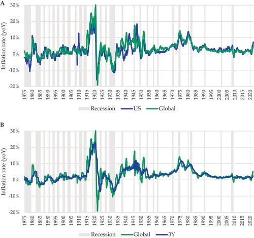
It is unlikely that investors care about transitory spikes in inflation that are expected to reverse in the next year when they price assets with long-term cash flows such as equities and bonds. Therefore, Figure 1B shows the rolling 3-year global inflation rate in addition to the annual global inflation rate. This figure again shows that before World War I, inflation was noisier and averaging over longer periods of time reduces the volatility of inflation substantially. However, after World War I, averaging has limited effect, as inflation and deflation spikes tend to be more persistent.

Table 1 summarizes the distribution of inflation over our sample. Panel A buckets global inflation into four inflation regimes: (1) below 0%, or deflation, (2) between 0% and the current central bank target of 2%, (3) a mild inflation overshoot, between 2% and 4%, and (4) high inflation, above 4%, and reports the number of years of inflation observations in each bucket. The midpoint between (2) and (3) was chosen because 2% is the current target of many central banks in major developed markets. As such, we focus on periods of negative inflation, inflation that realizes low relative to “target” (0–2%), inflation that overshoots the target (2–4%)—in 2021 an inflation level of 3% was seen by several investors as a material worry⁶—and inflation that is substantial (>4%).

Table 1. Inflation Frequencies

A. Global inflation episodes
Inflation bucket	1992–2021	1950–2021	1926–2021	1875–2021
<0%	0.9	1.6	7.7	23.1
0%–2%	20.3	25.5	27.6	42.9
2%–4%	8.6	22.7	25.9	34.9
>4%	0.3	22.3	34.8	46.1
All	30.0	72.0	96.0	147.0
B. U.S. inflation episodes
Inflation bucket	1992–2021	1950–2021	1926–2021	1875–2021
<0%	1.2	2.7	11.2	27.6
0%–2%	10.3	21.5	26.3	42.0
2%–4%	16.8	27.5	32.3	40.3
>4%	1.8	20.3	26.3	37.2
All	30.0	72.0	96.0	147.0
C. Inflation distribution
Inflation (YoY)		Percentile
	0.05	0.10	0.25	0.33	0.50	0.67	0.75	0.90	0.95
Global	–3.0%	–1.4%	1.0%	1.5%	2.3%	3.8%	4.6%	8.9%	12.1%
U.S.	–4.1%	–2.4%	0.2%	1.2%	2.2%	3.2%	4.1%	7.2%	11.2%

Notes: The table represents the historical distribution of inflation. Panel A (B) shows the average number of annual observations over different sample periods falling in each year-over-year (YoY) inflation level bucket based on global (U.S.) inflation. Panel C contains the distribution of global and U.S. inflation over the full sample, 1875–2021.

Over the entire sample period (1875–2021), there have been 23.1 years of deflation and 46.1 years with inflation above 4%. The subperiod analysis also shows that examining the most recent 30 years does not yield much information about deflationary or high-inflation periods, as inflation has almost always been in the range of 0% to 4%. Including the 1970s gives a period of high inflation, but one needs to include the 1930s to also have a substantial number of deflationary periods. Extending the sample to 1875 increases both the number of years with high inflation during and after World War II and with deflation at the end of the 19th century. Hence, extending the period to 1875 gives a more reliable assessment of what investors can expect during periods of deflation or high inflation. Panel B confirms these insights for U.S. inflation. Panel C contains more information about the distribution of inflation. The median value of annual inflation equals 2.3% for global and 2.2% for U.S. inflation. At the 10th percentile, there is a –1.4% and –2.4% deflation, respectively. At the other end, the 90th percentile is an inflation of 8.9% and 7.2%, respectively. Further, between 19% (deflation) and 29% (0%–2% inflation) of observations fall within each inflation regime when looking at U.S. inflation numbers.

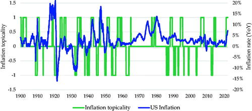
Central banks existed for most of our sample period. The U.S. Federal Reserve was founded in 1913, the Bank of England in 1694, the German Bundesbank in 1957 (its predecessor in 1948 and before World War II the Reichsbank in 1876), and the Bank of Japan in 1882. Their mandate to curb inflation to a predetermined level is a relatively recent phenomenon, mostly introduced after the inflation shocks in the 1970s. Explicit inflation targeting only started in the 1990s (see Svensson, 2011). Hence, we have to leave the impact of inflation targeting policies on the relationship between inflation and asset returns open. The lack of inflation targeting by central banks does not mean that investors did not care about deflation or inflation when judging stock and bond markets. This follows from a simple count of words measure of inflation- and deflation-related words as mentioned in the Abreast of the Market columns of The Wall Street Journal and related market commentary columns in The New York Times as used by Garcia (2013), which we acquire between 1899 and 2021. Figure 2 shows the relative importance of inflationary minus deflationary words per rolling annual window, computed by the standardized relative word frequencies.⁷ A value of 1 (–1) indicates inflation (deflation) words were commonly mentioned during that year in the market commentaries (i.e., they were “topical”, while a value of 0 indicates less investor consideration of inflation. This figure shows that before the inflation spikes in the 1970s, inflation was an important finance topic during periods with elevated inflation, and deflation was topical in deflationary periods. When regressed on U.S. inflation, the R² equals 51%. This evidence indicates that market participants were indeed aware of increases and decreases of consumer prices and linked it to asset prices.

Figure 2. Inflation Topicality

Notes: The figure shows the historical time-series behavior of inflation topicality (the relative mentioning of inflation versus deflation words in the market columns in The Wall Street Journal and/or The New York Times) versus U.S. year-over-year inflation. The sample period is 1899 to 2021.

Long-Run Evidence on Asset Class and Factor Premiums: 1875–2021

In this section, we examine asset class returns and factor returns within and across asset classes over our deep sample. Our dataset is at the monthly frequency and includes global equities, bonds, and cash returns; equity factor returns (Value, Momentum, Low Risk, and Quality); government bond factor returns (Value, Momentum, Low Risk, and Carry); and global factor returns (Value, [Time-Series] Momentum, Low Risk, and Carry) all expressed in USD. Our sample of returns and inflation numbers starts in January 1875, the first year we have global inflation series, and ends in December 2021. We include data on Value, Momentum, Low Risk, and Quality equity factors in the cross-section of U.S. stocks. These factors are the common factors employed in the industry, being the key motivation of our choice.⁸ Further, we consider U.S. stocks, as data on equity factors across the globe only starts toward the end of the 1980s. For global government bond market factors, we use data from Baltussen, Martens, and Penninga (2021) on Value, Momentum, Low Risk, and Carry factors, which we update until the end of December 2021. Finally, global (“cross-asset”) factor returns on Value, Momentum, Low Risk, and Carry are taken from Baltussen, Swinkels, and Van Vliet (2021), which we also update until the end of 2021.⁹ They construct GFPs using bond, equity, currency, and commodity market data at the country level, so no individual stocks. Appendix A.1 describes the data and factors that are used throughout the paper in detail.

We start our analysis by examining the long-run evidence on global asset class and factor returns. Table 2 contains the average returns on each of these asset classes and factor premiums over the long-run sample from 1875 to 2021, as well as several subsamples that start later. The reason to include these shorter subsamples is that they are often employed in earlier studies, thereby proving a form of “in-sample” evidence, while the longer-run evidence reveals the “out-of-sample” robustness of the asset class and factor premiums (although we leave a full out-of-sample study to the original papers with deep history). Moreover, those who find that the recent history is more representative of the future may be interested in more recent subsamples, even while these contain less powerful information about inflationary regimes.

Table 2. The Long-Run Evidence on Asset Class and Factor Premiums

	1992	1950	1926	1875	t value	Alpha	t value
	2021	2021	2021	2021
A. Asset classes
Equities	8.9**	12.1**	10.6**	8.4**	7.4	–	–
Bonds	5.4**	5.6**	5.1**	4.5**	14.0	–	–
Cash	2.3**	4.0**	3.2**	3.4**	40.4	–	–
60/40	7.5**	9.5**	8.4**	6.8**	9.5	–	–
B. Equity factors
Value	1.6	3.3**	4.0**	3.5**	3.0	3.9**	3.3
Momentum	5.4	8.2**	7.7**	6.9**	4.8	8.5**	6.0
Low Risk	6.4*	6.9**	6.0**	6.5**	6.7	5.0**	4.9
Quality	3.2**	2.9**	2.5**	2.5**	4.9	3.2**	6.0
MFE	4.1**	5.3**	5.2**	5.1**	7.4	5.5**	7.9
C. Bond factors
Value	0.8	4.0**	3.4**	2.4*	2.5	2.1	1.8
Momentum	2.4	2.6*	1.7	3.9**	3.9	4.2**	3.6
Low Risk	0.9	4.3**	4.5**	4.4**	4.0	6.1**	5.0
Carry	5.5**	7.9**	6.6**	7.4**	7.9	7.4**	6.8
MFB	2.4*	4.7**	3.9**	4.6**	9.4	4.9**	9.2
D. Global factors
Value	2.6**	2.7**	2.4**	2.3**	4.8	2.6**	4.8
Momentum/Trend	4.8**	7.3**	7.4**	7.4**	13.8	7.6**	12.6
Low Risk	0.7	2.2**	2.1**	1.6**	4.3	1.4**	3.5
Carry	5.5**	6.5**	4.9**	5.5**	11.4	5.3**	9.7
GFP	3.4**	4.7**	4.2**	4.2**	17.7	4.2**	15.7

Notes: The table shows historical returns on asset class and factor premium portfolios over various sample periods. Equity and bond returns are based on global portfolios, cash on short-dated U.S. cash investments. 60/40 represents a 60% equity, 40% bond portfolio. Equity factors: Quality starts in 1940, all other series in 1875. MFE takes an equally weighted combination of the equity factor premiums. Bond factors: Low Risk starts in 1922, all other series in 1875. MFB takes an equally weighted combination of the bond factor premiums. Global factors: All series start in 1875, composed of equal volatility weighted combinations of the factor premiums in equity indices, government bonds, currencies, and commodity futures. GFP takes an equally weighted combination of the global factor premiums. Alphas are relative to equity and bond asset class returns. Significant average returns at the 5% significance level are denoted with a * and significance at the 1% significance level with **. Numbers within parentheses represent t values. Standard errors are computed using the Newey–West procedure.

Panel A contains the returns on the conventional long-only asset classes equities, government bonds, and cash, and a multi-asset portfolio that consists of 60% equities and 40% government bonds.¹⁰ Long-term nominal average returns for global equity investors have been on average 8.4% per annum, a number that is high and significant (t value = 7.4).¹¹ Hence, equities offered an attractive return over 147 years. For sample periods that start later, average returns are also consistently positive ranging from 8.9% (1992–2021) to 12.1% (1950–2021) per annum.

Global (currency risk hedged) government bond returns have been substantially below global equity market returns with 4.5% per annum, but still significantly above zero (t value 14.0). This compares to an average return on cash of 3.4% per annum, while global inflation has been on average 3.2% per annum over the same period (see Table 1).¹² Hence, the global term premium is 1.1% per annum. Although this may appear to be modest, this may be partially due to the lack of a good proxy for the short-term risk-free rate over the long historical period, which may overstate the cash returns. For example, U.S. Treasury bills were not regularly issued until December 1929, when the auctioning of 13-week bills started. Most studies use commercial paper with 2 to 3 months’ maturity to proxy the short-term interest rate before the issuance of Treasury bills or certificates, but these contain a small credit premium relative to government issued securities.¹³ Consequently, we choose to focus our analysis on total asset class returns (instead of excess returns over cash).

In panel B, the four equity factors show strong and statistically significant performance over the long-run sample, with average returns ranging between 2.5% (Quality) to 6.9% (Momentum). Low Risk has the highest t statistic (6.7). The overall multi-factor equity (“MFE”) strategy, constructed as an equally weighted combination of the individual factors available each period, gives a robust and significant outperformance over each sample period. The average return since 1875 equals a statistically significant 5.1% with a high t value of 7.4. The average return is economically and statistically significant in all subsamples and is 4.1% over the most recent 30 years. During this more recent period, the Quality factor is somewhat stronger, with 3.2% per annum versus 2.5% in the longest sample that for Quality goes back to 1940 because no reliable accounting data are available before that time. Furthermore, the combination of Value and Momentum gives more consistent results than the individual strategies profiting from negative correlation between these two factors.¹⁴ When we correct for asset class risks, all equity factors remain significant in economic and statistical terms. Momentum and Low Risk have the highest alphas of 8.5% and 5.0% per annum, respectively, while Value and Quality have alphas exceeding 3%. The combined MFE alpha equals 5.5%, with a high t value of 7.9. In other words, equity factors are economically sizable and statistically robust phenomena over the last 147 years.

Panel C shows that results for bond factor premiums are similar. Value yields a statistically significant 2.4% per annum return (t value, 2.5), while Carry is the strongest factor, with an average return of 7.4% per annum (t value, 7.9). Further, the individual bond factors are generally sizable and statistically significant over most subsamples. The major exception is the most recent subperiod, in which Carry factor is the strongest factor with 5.5% return per annum, while the three other factors are positive but statistically indistinguishable from zero. However, due to diversification benefits across factors, the equally weighted multi-factor bond (“MFB”) strategy is statistically significant, with a return of 2.4% over the most recent 30 years. Over the full sample period, the MFB strategy returns a sizable 4.6% return, with again a high t value of 9.4, highlighting its robustness and statistical significance. As for equity factors, market risk adjustments in the final columns indicate that market risk is unable to explain any of the factors to a meaningful extent, and alpha is both sizable and significant for the MFB combination (4.9% per annum with a t value of 9.2).

Finally, GFPs are also sizable and highly significant, as shown in panel D. The Low Risk factor is the weakest among the factors, but it still shows an economically and statistically significant premium of 1.6% per annum (t value, 4.3).¹⁵ Momentum is the strongest over the sample since 1875 with an average return of 7.4% per annum (t value, 13.8). The equally weighted multi-factor GFP strategy returns 4.2% per annum, with an extremely high t value of 17.7. The four GFPs combined are economically and statistically significant over the various subsamples highlighting their robustness. Asset class risks cannot explain the global factor returns, witnessing alphas between 1.4% (Low Risk) and 7.6% (Momentum) and t values between 3.5 and 12.6. As for equity and bond factor premiums, market risk is not able to explain any of these GFPs, with an average alpha of 4.2% per annum (t value, 15.7) between 1875 and 2021. In sum, asset class (i.e., equities and bonds) and equity, bond, and GFPs are economically sizable and statistically significant and robust phenomena over the last 147 years.

Investment Returns During Deflationary and High-Inflation Periods

In this section, we examine the performance of asset classes and factor premiums over inflationary regimes. Our key focus is on the four inflationary regimes (<0%, 0%–2%, 2%–4%, and >4%) defined previously, but we like to stress that we consider robustness to other regime classifications as well. The first question to answer is the impact of inflation on returns of the three major asset classes (equities, bonds, and cash). Panels A1 and A2 of Table 3 contain the nominal and real returns of these asset classes over the full period as well as during the four inflation regimes defined above. We also include a multi-asset portfolio that consists of 60% equities and 40% bonds. This global portfolio returned 6.8% per annum in nominal terms (see also the previous section) and in 3.5% in real terms over the full sample period 1875 to 2021.

Table 3. Investment Returns by Inflation Regime

		Inflation Bucket
	All	<0%	0%–2%	2%–4%	>4%	Wald
Years	147	23.1	42.9	34.9	46.1	–
Likelihood (%)	100	15.7	29.2	23.7	31.4	–
Inflation (%)	3.2	–3.1	1.2	2.8	8.5	–
A1. Asset classes (nominal return)
Equities	8.4	2.4	11.1	11.0	6.9	3.9**
Bonds	4.5	5.2	4.7	4.5	3.9	0.6
Cash	3.4	2.8	2.7	3.4	4.2	3.5*
60/40	6.8	3.5	8.5	8.4	5.7	3.0*
A2. Asset classes (real return)
Equities	5.1	5.5	9.8	8.2	–1.7	4.2**
Bonds	1.2	8.4	3.4	1.6	–4.6	24.9**
Cash	0.1	5.9	1.5	0.5	–4.3	37.0**
60/40	3.5	6.7	7.2	5.6	–2.9	6.5**
B. Equity factors
Value	3.5	4.2	3.0	2.4	4.5	0.5
Momentum	6.9	5.9	6.1	7.4	7.7	0.3
Low Risk	6.5	7.0	7.4	5.3	6.2	0.3
Quality	2.5	3.6	3.3	2.2	2.0	0.5
MFE	5.1	5.9	5.1	4.5	5.3	0.4
C. Bond factors
Value	2.4	0.8	2.0	0.9	4.8	1.7
Momentum	3.9	5.6	5.0	6.0	0.4	2.7*
Low Risk	4.4	10.3	2.2	3.0	5.8	2.2
Carry	7.4	7.8	7.7	8.5	6.1	0.5
MFB	4.6	5.3	4.7	4.9	4.0	0.4
D. Global factors
Value	2.3	1.2	3.3	1.9	2.1	1.8
Momentum/Trend	7.4	6.8	7.4	5.7	8.9	2.9*
Low Risk	1.6	1.0	1.1	2.1	2.0	1.2
Carry	5.5	4.7	6.0	7.1	4.3	2.4
GFP	4.2	3.4	4.4	4.2	4.3	1.3
E. Assets + Factors (real return)
Equities + MFE	7.7	8.5	12.4	10.4	1.0	4.1**
Bonds + MFB	3.5	11.0	5.7	4.1	–2.6	21.3**
Cash + GFP	4.3	9.3	5.9	4.7	0.0	24.5**
60/40 + All factors	6.9	10.2	10.6	8.7	0.4	6.3**

Notes: The table shows historical returns on asset classes and factor premiums bucketed by four contemporaneous global inflation categories (from deflation, <0%, to high inflation, >4%). The sample period is 1875 to 2021. Returns are in percentages per annum. Significance at the 5% significance level is denoted with * and significance at the 1% significance level with **. A Wald F test is used to test for significant average return differences across the different inflationary states. All standard errors are computed using the Newey–West procedure. In panel E, we proxy a long-only investment with a 100% allocation to the market and a 50% allocation to the long-short multi-factor premium strategy in that asset class.

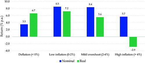
Deflationary periods, where inflation is below 0%, coincide with relatively low nominal returns for equities of 2.4% per annum, well below the 8.4% unconditional average return. Bonds and cash show a 5.2% and 2.8% per annum nominal return during deflationary periods, respectively, which is slightly above the unconditional averages of 4.5% and 3.4%. Consequently, a multi-asset 60/40 investor achieved a 3.5% nominal return during deflationary periods. However, an investor that does not suffer from money illusion realizes that even though the nominal return is low, the real return is decent because of the deflation. Adjusted for purchasing power, the multi-asset investor earns 6.7% per annum during deflationary periods.

High inflation periods, where inflation is above 4%, show a positive nominal return for equities (6.9%) and bonds (3.9%). At face value, it may seem that the multi-asset investor does quite well with a 5.7% nominal return. However, the real return is substantially negative at –2.9% per annum, leading to a severe reduction in purchasing power.

The two periods in between, with a positive inflation just below current central bank targets of 2% and a mild overshoot of those targets to 4%, are both good for equities and bonds, with nominal returns on equities of 11.0%, well above their unconditional average, and nominal returns on bonds in line with their unconditional average. In real terms, returns on these asset classes are also good, with the undershoot scenario being even somewhat better with a 9.8% real return for equities and 3.4% for bonds. The real return on the 60/40 multi-asset portfolio is 7.2% and 5.6% per annum for the 0%–2% and 2%–4% inflation buckets. In other words, positive but low consumer price increases are good for nominal investment returns, as well as those adjusted for purchasing power.

The last column summarizes the results of a Wald test (adjusted for serial correlation due to the use of 12 months’ overlapping observations) that tests whether the variation of returns across inflation scenarios is statistically significant. Nominal equity, cash, and multi-asset returns vary significantly across inflationary regimes, while the variation in nominal bond returns is not significant. Because of the huge differential of average inflation during the inflation scenarios, the variation in real returns is significant for all asset classes.

Figure 3 summarizes these insights by depicting the average nominal and real annual return on the multi-asset portfolio across the inflationary regimes. Inflation just below or above the inflation target of 2% is good for investors in both nominal and real terms. Deflation is relatively bad for nominal returns, but good in real terms. Nominal returns during periods with high inflation seem acceptable but in real terms are dramatically negative.

Figure 3. Nominal and Real 60/40 Returns across Inflation Regimes, 1875–2021

Notes: The figure shows the historical average nominal return (grey bars) and real return (black bars) on the 60/40 global equity/bond portfolio across inflationary regimes. The sample period is 1875 to 2021.

As outlined in the previous section, factor premiums offer significant and diversifying returns over asset class premiums. Many investors distinguish factor premiums in their strategic asset allocation, and it therefore is of interest to examine the variation in factor premiums across inflationary regimes. Panels B, C, and D in Table 3 show the factor returns for each of the four inflation buckets. Interestingly, the factor performances do not seem to depend much on the level of inflation, in contrast to the asset class returns. Indeed, the multi-factor equity portfolio performs at 5.9% in deflation, 5.3% in inflationary periods, and 5.1% and 4.5% when inflation is just below or above the central bank targets, respectively. Variations across inflation buckets at the individual factor level are somewhat higher but remain quite close to their unconditional averages. The Wald tests indicate that the observed variation across inflation scenarios is not statistically significant, even for some factors sometimes believed to vary with inflation such as Momentum and Value. These findings for Value, Momentum, and Quality generally align with the findings of Neville et al. (2021) over a shorter sample and with a different inflation definition.¹⁶

Bond factors also deliver positive returns across all four inflationary regimes, although they generally perform in a more mixed way across the regimes. Value in bonds is performing well when inflation is high (4.8%), but not in deflationary periods (0.8%). That said, its return variations across regimes are insignificant as reflected in the Wald test. Momentum in bonds, on the other hand, is performing well in each period (5.6%, 5.0%, and 6.0%) except when inflation is high (0.4%), and its variation across inflationary regimes is significant. The Low Risk factor performs especially well in times of deflation (10.3%, compared to a 4.4% unconditional average) and inflation (5.8%), but again return variations across regimes are not significant. Further, the Carry factor is not much affected by inflation regimes. As for equities, the multi-factor bond portfolio performs consistently high across inflation regimes, delivering positive returns in each inflationary regime.

The GFPs also deliver positive and consistent returns across all four inflationary regimes. Seemingly, Value has lower returns during deflationary periods with 1.2% per annum, but the Wald test fails to reject the null hypothesis of no significant return variations across the four inflationary regimes (Time-Series). Momentum varies significantly across the regimes, as it performs best during periods with high inflation (8.9% per annum), which is consistent with the findings of Neville et al. (2021) who examine the post-1926 period. However, it delivers positive returns on average across all four regimes. Low Risk performs above average when inflation is above 2% but does not display significant return variation across regimes. Carry also delivers positive and fairly similar average returns across the regimes. Similar to the equity and bond factors, the multi-factor strategy in the multi-asset universe is virtually immune to inflation or deflation shocks, at least on average, with excess returns ranging from 3.4% to 4.4% per annum.

The factor returns are the return differential between a long portfolio with the highest factor exposures and a short portfolio with the lowest factor exposures. The excess returns on these “zero investment” portfolios are therefore the same in nominal and real terms. In practice, an investor would need to hold either a cash position to fund these long-short strategies, for example, as a derivatives-based overlay on top of the conventional asset allocation, or replace the conventional asset allocations to equities and bonds with the long side of each factor. It depends on the nature of the factor, the trading costs involved with different instruments, and the investor’s willingness and ability to deal with derivatives what an optimal implementation in practice would be.

Panel E considers these portfolio implementations. For equities, we replace its “passive” allocation with an approximate long-only allocation to the multi-factor equity strategy. Similarly, for bonds we replace its “passive” allocation with an approximate long-only allocation to the multi-factor bond strategy.¹⁷ We add the GFP strategy, which represents a long-short strategy in derivatives across the major global markets, to the cash portfolio to generate a factor-based absolute return macro strategy. We see that the multi-factor long-only equity investor can increase their full sample real return from 5.1% to 7.7% per annum, the long-only bond investor from 1.2% to 3.5%, the cash investor from 0.1% to 4.3%, and the 60/40 multi-asset portfolio from 3.5% to 6.9% per annum, assuming that the GFP is added via an overlay on 20% of the portfolio’s value. Further, the long-only factor strategies consistently add across inflationary regimes, with for example the factor-enhanced equity (multi-asset) allocation managing to make up for the losses of the conventional portfolio in the high-inflation regime, as its average real return equals 1.0% (0.4%).

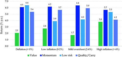
The factor premiums averaged across equity, government bonds, and the GFPs for each of the four inflationary regimes are displayed in Figure 4. The Value factor is the weakest stand-alone (while diversifying well to the other factors; see, for example, Baltussen, Swinkels, and Van Vliet 2021), but performs relatively well during high-inflation periods when conventional asset classes do poorly. On the other hand, Quality/Carry perform slightly worse during inflationary times, but better in each of the other inflationary regimes. Low Risk performs well especially in the extremes, that is, deflationary, or high-inflation regimes, and is weaker in the middle two that are goldilocks scenarios for equities and bonds. Finally, Momentum performs consistently and well across the inflationary regimes.

Figure 4. Factor Premiums across Inflation Regimes, 1875–2021

Notes: The figure shows the historical average return on Value, Momentum, Low Risk, and Quality/Carry factor premiums across inflationary regimes. Factor premiums are computed as the equally weighted average of equity, government bond, and global factor premiums. The sample period is 1875 to 2021.

Over longer-term horizons, the risk of equities, bonds, and factor premiums can be different. For example, Ely and Robinson (1997) and Schotman and Schweitzer (2000) show that equities offer better inflation protection over the long term. Table 4 shows the same results as Table 3, but now moving from a 1-year to a 3-year evaluation horizon. This hardly affects the observation frequency of each of the regimes. The deflation regime occurs 14% of the time (16% for 1 year), in which the 60/40 portfolio offers the highest annualized real return across each of the regimes. During a high-inflation regime (>4%) the annualized real equity return is still negative, even somewhat lower than on a 1-year evaluation horizon. This is contrary to the hypothesis that equities offer higher real returns on longer investment horizons.¹⁸ The equity, bond, and GFPs remain stable across the different inflation regimes.

Table 4. Inflation Regimes with 3-Year Investment Horizon

		Inflation Bucket
	All	<0%	0%–2%	2%–4%	>4%	Wald
Years	147	21.0	47.8	36.3	41.9	–
Likelihood (%)	100	14.3	32.5	24.7	28.5	–
Inflation (%)	3.2	–2.2	1.4	2.9	8.3	–
A1. Asset classes (nominal return)
Equities	8.2	4.7	9.5	12.3	5.5	2.5
Bonds	4.5	4.6	4.1	5.1	4.3	0.6
Cash	3.4	3	2.7	3.8	4.1	1.8
60/40	6.7	4.6	7.3	9.4	5.0	2.1
A2. Asset classes (real return)
Equities	5.0	6.9	8.1	9.4	–2.7	3.1*
Bonds	1.3	6.8	2.6	2.2	–3.9	17.1**
Cash	0.2	5.2	1.3	0.9	–4.2	25.4**
60/40	3.5	6.9	5.9	6.5	–3.2	4.5**
B. Equity factors
Value	3.6	6.5	2.2	2.8	4.5	1.2
Momentum	6.9	7.2	5.4	8.4	7.1	1.2
Low Risk	6.4	7.0	6.7	7.3	4.8	0.6
Quality	2.5	–	3.1	2.5	1.8	0.6
MFE	5.2	7.0	4.6	5.5	4.6	1.0
C. Bond factors
Value	2.4	1.1	0.9	2.4	4.7	2.2
Momentum	4.0	5.6	5.2	5.7	0.3	2.1
Low risk	4.3	8.9	1.3	4.7	5.8	3.0*
Carry	7.5	7.8	7.4	9.0	6.1	0.8
MFB	4.6	5.3	4.2	5.7	3.7	1.5
D. Global factors
Value	2.3	0.8	2.3	2.5	2.8	1.6
Momentum/Trend	7.4	7.7	6.8	6.5	8.7	1.1
Low Risk	1.6	0.7	0.7	2.7	2.0	2.7*
Carry	5.6	4.4	5.8	7.2	4.4	2.2
GFP	4.2	3.4	3.9	4.7	4.5	2.2
E. Assets + Factors (real return)
Equities + MFE	7.6	10.4	10.4	12.2	–0.4	3.1*
Bonds + MFB	3.6	9.5	4.7	5.1	–2.1	15.2**
Cash + GFP	4.4	8.6	5.2	5.6	0.3	7.8**
60/40 + All factors	6.8	10.7	8.9	10.3	–0.2	4.4**

Notes: The table shows historical returns on asset classes and equity, bond, and global macro-factor premiums bucketed by four global inflation categories (from deflation, <0%, to high inflation, >4%) using a 3-year inflation classification and investment holding period. The sample period is 1875 to 2021. Returns are in percentages per annum. Note that for equity Quality, which starts in 1940, no 3-year deflationary observations are available. Significance at the 5% significance level is denoted with * and significance at the 1% significance level with **. A Wald F test is used to test for significant average return differences across the different inflationary states. All standard errors are computed using the Newey–West procedure.

In Appendix A.2, we show that the results are robust across (i) different definitions of inflationary regimes, including a 3% or 5% (instead of 4%) high inflation cutoff, (ii) the use of annual changes in inflation rates (as measure of unexpected inflation), (iii) the use of only U.S. (instead of global) inflation, and (iv) across the first (i.e., 1875–1948) and second half (i.e., 1949–2021) of our sample period. Noteworthy observations include poorer nominal and real global equity returns the higher the high inflation cutoff and stronger returns on equity factors (especially Momentum and Low Risk) and stronger returns on two value factors (Bond Value and Global Value) during times of falling inflation. During times of strongly rising inflation, Equity Momentum and Global Momentum (Trend) have higher returns. Finally, the results are robust across two subsamples with some noteworthy observations. During the early period from 1875 to 1948, bonds are doing even worse during inflationary periods, both in nominal and real terms, whereas Bond Momentum shows low but positive returns. Note that in our second sub-period, 1949 to 2021, there are less than 2 years with deflation observations, which is not sufficient for reporting meaningful average realized returns. In general, factors premiums are robust across the two subsamples offering positive returns across the different inflationary regimes.

In sum, our findings show that asset class premiums vary significantly across the inflationary regimes in nominal and especially real terms. Equities and bonds on average yield lower nominal returns during periods of high inflation, causing negative real returns. By contrast, equity, bond, and GFPs are generally positive across high-inflation regimes, displaying generally limited variation across, while they enhance nominal and real asset class returns in (approximated) long-only asset class implementations. These results suggest that equity and bond market premiums could be explained by offering a compensation for inflation risk, while factor premiums cannot. This leaves room for further research into other explanations as to why factor premiums exist. A portfolio implication is that a balanced exposure to multiple factor premiums is difficult to beat with dynamic factor timing based on inflationary cycles.¹⁹

Dissecting Inflationary Regimes: Stagflation Hurts

In the previous section, we observed that real returns during inflationary periods are negative for investors in stocks and bonds but that equity, bond, and GFPs are mostly resilient during different inflation scenarios. In this section, we further split up the “bad times” of high-inflation episodes as well as deflationary periods based on other economic or financial market circumstances. Not all inflationary regimes are alike, and hence the question is how investment returns behave over various sub-regimes within high-inflation and deflationary regimes.

To this end, we divide the periods based on five different characteristics: (1) recession or expansion, (2) falling or rising earnings growth, (3) bear or bull equity markets, and (4) increasing or decreasing interest rates, and (5) increasing or decreasing inflation. This includes stagflationary episodes with both high inflation and recessions. We date recessions based on business cycle data from the National Bureau of Economic Research²⁰ by requiring that at least six of the months in a rolling 12-month window are classified as recession.²¹ In total, there have been 30 recessions over the period 1875 to 2021 with an average duration of 17 months. We define increasing or decreasing interest rates based on the sign of the 12-month change in global government bond rates and a bull (bear) equity market based on the sign of global equity returns.

The average returns per high inflation sub-regime are displayed in Table 5. Panel A1 (A2) of Table 5 shows that nominal (real) returns on equities are particularly bad during recessions with high inflation, or stagflationary episodes. The nominal (real) return on the multi-asset portfolio is –2.2% (–11.7%) per annum, compared to 8.2% (–0.1%) during expansionary periods with high inflation. Recessions likely lead to lower expected corporate cash flows, which dominate a decrease in the discount rate, leading even to negative nominal stock returns of –7.1% per annum. Recessionary periods are somewhat better for nominal bonds than expansionary periods with nominal returns of 5.1% versus 3.6% per annum. Decreasing interest rates lead to positive marked-to-market gains. The negative real return for equities of –16.6% suggests that equities are a particularly bad inflation hedge during stagflationary periods. While expansionary periods in general tend to be good for investors, this does not hold when inflation is high. Real returns on stocks are marginally positive (2.9% per annum) and real returns on bonds are deeply negative (–4.7%). Even though the economy is doing well, times of high inflation are generally not good for investors.

Panels B, C, and D contain the result of the factor premiums and give a completely different picture. The multi-factor equity portfolio has a return of 5.4%, the multi-factor bond portfolio 4.7%, and the GFP portfolio a return of 4.1% during stagflation periods. If anything, the stagflation performances for factor premiums in equities and bonds are even better than during expansions in high-inflation periods, albeit not statistically significantly different (unreported). All factor premiums perform well during stagflations except for Momentum in bonds, which returns –2.4% on average. Similarly, GFPs perform well, with only Low Risk returning zero and all other factors returning positively.

Panel E of Table 5 also show that investors who are, for example, worried about achieving negative real returns during stagflation periods may improve their asset allocation by including factors across asset classes. This would help their portfolio to a certain extent from these adversary business cycle conditions. Even though –8.3% per annum in real terms can hardly be called a success, it is substantially better than the alternative of –11.7% per annum. Note that the factor series are all long-short factors that do not include trading costs, and investors need to construct efficient ways to exploit these factor strategies in practice.

The NBER definition of a recession is based on negative GDP growth, but we also examine declining (annual) earnings of the stock market (based on data from Shiller’s website), as that part of the economy may be more relevant for equity investors. Real returns on the multi-asset portfolio remain poor, although better than during NBER stagflations, with –5.8% versus –11.7%. The MFB premiums are positive, but relatively low with 2.5%, because Momentum and Carry have relatively low returns. MFE and GFP show average returns, leading to a –3.2 real return on a multi-asset portfolio that includes factors.

Decreasing equity markets in periods with high inflation are especially disastrous with an annualized real return of –28.8%. At the same time, bonds suffer in real terms during high inflation and falling equity market episodes with –9.0% per annum negative real returns, yielding a –20.9% real return on the multi-asset portfolio. For both bear and bull equity markets in times of inflation, a diversified portfolio of factor premiums yields robust performance enhancements, thereby alleviating the pain of high inflation. Again, all factor premiums yield positive returns, except for Momentum in bonds and Low Risk across assets during high inflation bear markets.

When we sub-condition on changes in interest rates, it becomes clear that increasing interest rates cause more pain (real –6.8% per annum) to a conventional multi-asset portfolio than decreasing interest rates (real 2.2% per annum), as both equities and bonds suffer in real terms (–6.0% and –8.0% per annum, respectively). By contrast, during decreasing rate periods equities and bonds experience materially better real returns (3.9% and –0.3% per annum). Average returns on factor premiums are again good across sub-regimes, but generally a bit better during when rates increase. Especially Momentum in equities and Trend following stand out during these episodes, while Low Risk in equities and Value in bonds benefit more from declining rates in times of inflation. Again, factor premiums materially help to soften to burden of high inflation for traditional portfolios (Table 5).

Table 5. A Deeper Look at Returns During High-Inflation Periods

	High Inflation (>4%)
	NBER		Earnings		Equity		Rates		Inflation
	↓	↑	↓	↑	↓	↑	↑	↓	↑	↓
Years	10.9	35.3	16.8	29.3	12.8	33.4	25.9	20.1	28.5	17.6
Likelihood	23.4	76.6	36.5	63.5	27.8	72.2	56.2	43.8	61.8	38.2
Inflation (%)	9.5	8.3	9.8	7.8	10.8	7.7	9.0	8.0	9.1	7.6
A1. Asset classes (nominal return)
Equities	–7.1	11.2	3.2	9.0	–18.0	16.4	3.0	11.9	5.6	9.0
Bonds	5.1	3.6	5.0	3.3	1.8	4.7	1.0	7.7	2.4	6.4
Cash	5.4	3.8	4.6	4.0	4.3	4.2	4.7	3.6	3.8	4.8
60/40	–2.2	8.2	4.0	6.2	–10.1	11.7	2.2	10.2	4.1	7.5
A2. Asset classes (real return)
Equities	–16.6	2.9	–6.7	1.2	–28.8	8.7	–6.0	3.9	–3.5	1.4
Bonds	–4.4	–4.7	–4.8	–4.5	–9.0	–3.0	–8.0	–0.3	–6.8	–1.1
Cash	–4.1	–4.4	–5.2	–3.8	–6.5	–3.5	–4.3	–4.4	–5.3	–2.8
60/40	–11.7	–0.1	–5.8	–1.6	–20.9	4.0	–6.8	2.2	–5.0	0.0
B. Equity factors
Value	3.0	4.9	3.0	5.3	6.2	3.8	3.4	5.8	4.3	4.8
Momentum	7.2	7.9	7.3	8.0	8.0	7.6	10.0	4.8	8.7	6.1
Low Risk	7.6	5.8	6.1	6.4	5.6	6.5	4.9	8.0	4.7	8.8
Quality	4.6	1.4	2.7	1.6	3.1	1.6	2.5	1.4	1.9	2.2
MFE	5.4	5.2	4.8	5.5	5.7	5.1	5.3	5.1	5.1	5.5
C. Bond factors
Value	5.8	4.5	6.1	4.1	5.9	4.4	2.8	7.4	1.9	9.6
Momentum	–2.4	1.3	–3.8	2.9	–5.9	2.8	1.0	–0.2	1.7	–1.7
Low Risk	14.3	3.3	10.2	3.5	1.4	7.8	7.0	4.9	6.1	5.3
Carry	5.5	6.2	1.4	8.8	9.5	4.4	7.0	4.3	7.4	3.9
MFB	4.7	3.7	2.5	4.8	1.6	4.9	4.2	3.7	4.1	3.7
D. Global factors
Value	3.9	1.6	3.7	1.2	4.0	1.4	1.4	3.1	1.4	3.3
Momentum/Trend	7.3	9.4	8.0	9.4	9.6	8.6	10.4	6.9	9.1	8.5
Low Risk	0.0	3.3	1.4	2.3	–0.3	2.8	1.9	2.1	1.7	2.5
Carry	5.2	4.1	3.1	5.0	2.8	4.9	5.0	3.5	5.2	3.0
GFP	4.1	4.6	4.0	4.5	4.0	4.4	4.7	3.9	4.3	4.3
E. Assets and Factors (real return)
Equities + MFE	–13.9	5.5	–4.3	4.0	–26.0	11.3	–3.4	6.5	–1.0	4.2
Bonds + MFB	–2.1	–2.9	–3.6	–2.1	–8.2	–0.6	–5.9	1.6	–4.8	0.8
Cash + GFP	0.0	0.2	–1.2	0.7	–2.5	0.9	0.4	–0.5	–1.0	1.5
60/40 + All factors	–8.3	3.1	–3.2	2.4	–18.1	7.4	–3.4	5.3	–1.6	3.7

Notes: The table shows historical returns on asset classes and factor premiums during high-inflation regimes, sub-bucketed based on recessions or expansion, increasing or decreasing corporate earnings, equity bull or bear markets, increases or decreases in long-term rates, or increases or decreases in 1-year inflation rates. The sample period is 1875–2021. Returns are in percentages per annum. NBER: National Bureau of Economic Research.

The final sub-regime is that of increasing inflation during periods in which inflation is above 4%. This happens in 28.5 out of 46.1 years. Nominal and real equity and bond returns are worse than during the average year in a high-inflation regime. Consequently, real returns on the multi-asset portfolio are –5.0%, worse than with decreasing inflation but not as bad as during stagflation periods. Again, factor premiums perform consistent and well, with government bond factor premiums being particularly high, mostly due to Low Risk and Carry outperforming. As before, a diversified portfolio of factor premiums yields robust performance enhancements, thereby alleviating the pain of high inflation. The robust results on factor investing do not mean that investing in factor premiums is without risk. For example, Blitz (2021) suggests that quant equity factors follow their own “quant cycle,” which is unrelated to business cycle variables that we examine here.

To test for consistency in returns, Table 6 shows the probability of a positive annual nominal return for each high inflation sub-regime. The probabilities are on a 0 to 100 scale in percentage. We have seen that average nominal equity returns are negative in a stagflation scenario, with also most observations returning negative and only 40.8% of all annual equity returns being positive. Panel B shows that the annual positive returns of the combined MFE equity factors vary between 76% and 85%. This means that the average premiums are positive and consistent across all high-inflation regimes. On an individual factor level, Quality is somewhat less consistent, with positive return rates below 50%. Momentum is most consistent, with positive return rates around 75%. Still, due to diversification benefits, the combination of factors offers more consistent positive returns than the best individual equity factor (Momentum). Panel C shows a similar consistent picture for bond factor returns: The average annual combined MFB returns are positive, with probabilities varying between 63% and 81%. The most consistent bond factor is Carry. Finally, the GFPs also show consistently positive annual returns during high-inflation regimes, with probabilities ranging between 87% and 95%. Neville et al. (2021) find that trend strategies offer good and consistent protection during high-inflation periods. In this more granular analysis within a wide range of high-inflation periods, Trend is again the most persistent factor, which extends and supports these earlier findings.

Table 6. A Deeper Look at Returns During High Inflation Periods: Frequencies

	High Inflation (>4%)
	NBER		Earnings		Equity		Rates		Inflation
	↓	↑	↓	↑	↓	↑	↑	↓	↑	↓
Years	10.9	35.3	16.8	29.3	12.8	33.4	25.9	20.1	28.5	17.6
Likelihood	23.4	76.6	36.5	63.5	27.8	72.2	56.2	43.8	61.8	38.2
Inflation (%)	9.5	8.3	9.8	7.8	10.8	7.7	9.0	8.0	9.1	7.6
A. Asset classes (nominal return)
Equities	40.8	82.0	65.3	76.4	0.0	100.0	67.2	78.9	74.3	69.2
Bonds	82.3	78.0	85.1	75.5	65.4	84.3	63.3	99.2	73.4	88.2
Cash	98.5	95.5	98.0	95.2	95.4	96.5	98.4	93.4	96.8	95.3
60/40	54.6	83.7	72.8	79.2	18.3	99.3	69.8	86.0	76.3	77.7
B. Equity factors
Value	57.7	67.1	62.9	66.1	69.3	63.3	59.8	71.5	64.0	66.4
Momentum	70.8	79.4	73.3	79.8	77.1	77.5	82.0	71.5	80.4	72.5
Low Risk	70.8	73.8	73.3	72.9	75.8	72.0	69.5	77.7	69.3	79.1
Quality	47.7	47.8	51.5	45.6	45.8	48.5	47.9	47.5	40.9	58.8
MFE	76.2	85.1	77.7	86.0	82.4	83.3	85.2	80.2	83.0	82.9
C. Bond factors
Value	56.9	64.3	60.4	63.8	58.8	64.0	60.1	65.7	54.7	75.4
Momentum	50.0	54.4	44.6	58.4	42.5	57.5	54.7	51.7	54.1	52.1
Low Risk	56.2	51.1	51.5	52.7	60.1	49.3	55.9	47.5	46.5	61.6
Carry	66.2	71.9	62.9	74.9	61.4	74.0	73.3	66.9	75.4	62.6
MFB	70.0	76.1	63.4	81.2	62.7	79.3	78.8	69.4	74.9	74.4
D. Global factors
Value	71.5	64.5	74.8	61.3	77.1	62.0	60.1	64.0	60.8	74.9
Momentum/Trend	89.2	91.7	89.1	90.2	87.6	92.5	95.5	85.5	92.7	88.6
Low Risk	29.2	72.6	63.4	61.8	41.8	70.3	58.5	67.4	61.4	74.0
Carry	77.7	72.3	69.8	75.8	66.0	76.5	79.1	66.5	81.0	61.6
GFP	87.7	95.5	92.6	94.3	89.5	95.3	93.6	93.8	93.9	93.4

Notes: The table shows historical frequencies of positive annual returns on asset classes and factor premiums during high-inflation regimes, sub-bucketed based on recessions or expansion, increasing or decreasing corporate earnings, equity bull or bear markets, increases or decreases in long-term rates, or increases or decreases in 1-year inflation rates. The sample period is 1875 to 2021. Frequencies are expressed in percentages per annum. NBER: National Bureau of Economic Research.

Next, we examine performances over deflationary sub-regimes, as shown in Table 7. The total deflationary period is 23.1 years, about half of the 46.1 years that have inflation above 4%. This means that the sub-regimes are sometimes small, with several of them having less than 10 years of observations, reducing the accuracy of the displayed averages. Deflationary expansions are relatively good for investors, with a 10.4% real return per annum for the 60/40 portfolio, while deflationary recessions are slightly positive (1.6%) in nominal terms, but better in real terms (4.9%). For the multi-asset investor, interest rate increases are worse than decreases (with equities returning negatively) and equity market bear markets worse than bull markets. Most troubling are deflationary episodes that coincide with equity bear markets. The equity, bond, and global factors multi-factor combinations do well for each of the sub-regimes during deflationary periods, especially equity and bond factors during the states with poor equity or bond returns—deflationary recession or bear markets. Further, individual factor performances vary, although we have to be cautious as some samples are fairly small. For example, equity Value does rather poorly during deflationary expansion periods (–4.5%) when equity Low Risk does particularly well (16.1%). The same holds for bond Value and, to a lesser extent, for Value across assets. The GFP portfolio does not vary a lot across sub-regimes, ranging between 2.3% and 4.1%. Overall, we observe that especially equity and bond factors perform tend to do well during the bad times in deflationary cycles but that these bad times are much milder than during stagflations.

Table 7. A Deeper Look at Returns During Deflationary Periods

	Deflation (<0%)
	NBER		Earnings		Equity		Rates		Inflation
	↓	↑	↓	↑	↓	↑	↑	↓	↑	↓
Years	15.8	7.3	14.6	8.5	8.2	14.9	6.4	16.7	6.1	17.0
Likelihood (%)	68.2	31.8	63.2	36.8	35.4	64.6	27.8	72.2	26.4	73.6
Inflation (%)	–3.3	–2.7	–3.7	–2.2	–3.9	–2.6	–2.7	–3.3	–2.7	–3.2
A1. Asset classes (nominal return)
Equities	–1.3	10.2	–0.6	7.5	–12.1	10.3	–4.3	4.9	11.1	–0.7
Bonds	4.9	5.9	5.5	4.8	4.1	5.9	1.7	6.6	5.9	5.0
Cash	3.0	2.6	2.9	2.8	2.9	2.8	2.8	2.8	2.6	2.9
60/40	1.6	7.7	2.2	6.0	–4.1	7.8	–1.2	5.4	8.2	1.9
A2. Asset classes (real return)
Equities	2.0	13.0	3.0	9.7	–8.2	13.0	–1.6	8.2	13.8	2.5
Bonds	8.2	8.6	9.1	7.0	8.1	8.5	4.4	9.9	8.6	8.2
Cash	6.3	5.3	6.5	4.9	6.9	5.4	5.5	6.1	5.3	6.2
60/40	4.9	10.4	5.8	8.1	–0.2	10.4	1.5	8.7	10.9	5.2
B. Equity factors
Value	8.3	–4.5	7.8	–2.0	8.0	2.1	14.1	0.4	7.1	3.2
Momentum	7.9	1.5	7.2	3.7	19.1	–1.4	13.1	3.1	–14.2	13.1
Low Risk	2.6	16.1	3.7	12.6	0.8	10.6	6.3	7.2	7.8	6.6
Quality	5.3	–0.1	3.0	4.2	6.6	2.4	4.4	3.0	–	3.6
MFE	6.7	4.3	6.7	4.6	9.7	3.9	11.2	3.9	0.2	8.0
C. Bond factors
Value	1.3	–0.3	1.9	–1.2	4.8	–1.4	2.2	0.3	–2.7	2.0
Momentum	5.6	5.5	5.4	5.9	6.4	5.1	10.1	3.9	1.6	7.0
Low Risk	12.2	7.2	12.5	6.1	15.0	6.8	2.7	11.9	7.6	11.3
Carry	8.6	6.2	7.7	7.9	9.0	7.2	9.3	7.2	6.1	8.4
MFB	5.7	4.4	5.7	4.6	7.6	4.0	7.0	4.6	2.1	6.4
D. Global factors
Value	2.0	–0.4	1.5	0.8	3.3	0.1	1.8	1.0	–3.0	2.7
Momentum/Trend	7.7	4.9	7.6	5.3	9.2	5.5	5.8	7.2	7.5	6.5
Low Risk	0.5	1.9	1.1	0.6	–0.6	1.7	0.8	1.0	3.6	0.0
Carry	5.5	2.9	4.3	5.3	4.3	4.9	4.2	4.9	3.3	5.2
GFP	3.9	2.3	3.6	3.0	4.1	3.0	3.1	3.5	2.9	3.6
E. Assets + Factors (real return)
Equities + MFE	5.4	15.2	6.4	12.0	–3.4	15.0	4.0	10.2	13.9	6.5
Bonds + MFB	11.1	10.8	12.0	9.3	11.9	10.5	7.9	12.2	9.7	11.4
Cash + GFP	10.2	7.6	10.1	7.9	11.0	8.4	8.6	9.6	8.2	9.8
60/40 + All factors	8.4	13.9	9.3	11.5	3.6	13.8	6.2	11.7	12.8	9.2

Notes: The table shows historical returns on asset classes and factor premiums during high-inflation regimes, sub-bucketed based on recessions or expansion, increasing or decreasing corporate earnings, equity bull or bear markets, increases or decreases in long-term rates, or increases or decreases in 1-year inflation rates. The sample period is 1875 to 2021. Returns are in percentages per annum. NBER: National Bureau of Economic Research.

To test for consistency in returns, Table 8 shows the probability of a positive annual nominal return for each deflation sub-regime. During a deflationary recession, equities have positive annual returns 50.8% of the time, whereas equities almost always go up with deflationary expansion periods (94.3%). The highest return on 60/40 is made during the deflation scenario when prices start to rise again. During these “good times,” the 60/40 portfolio has positive annual returns 94.5% of the time. The combined equity factors (MFE) tend to do well across most deflation regimes, as shown in panel B. The same applies for bond factors and global factors, as shown in panels C and D. This again confirms the diversification benefits of factor investing across inflationary regimes.

Table 8. A Deeper Look at Returns During Deflationary Periods: Frequencies

	Deflation (<0%)
	NBER		Earnings		Equity		Rates		Inflation
	↓	↑	↓	↑	↓	↑	↑	↓	↑	↓
Years	15.8	7.3	14.6	8.5	8.2	14.9	6.4	16.7	6.1	17.0
Likelihood (%)	68.2	31.8	63.2	36.8	35.4	64.6	27.8	72.2	26.4	73.6
Inflation (%)	–3.3	–2.7	–3.7	–2.2	–3.9	–2.6	–2.7	–3.3	–2.7	–3.2
A. Asset classes (nominal return)
Equities	50.8	94.3	50.9	88.2	0.0	100.0	50.6	70.0	86.3	56.9
Bonds	94.2	100.0	94.3	99.0	89.8	99.4	87.0	99.5	98.6	95.1
Cash	100.0	100.0	100.0	100.0	100.0	100.0	100.0	100.0	100.0	100.0
60/40	66.7	97.7	66.3	94.1	33.7	100.0	67.5	80.0	94.5	70.1
B. Equity factors
Value	61.9	40.9	60.6	46.1	66.3	49.2	73.5	47.5	57.5	54.5
Momentum	77.2	58.0	77.7	59.8	88.8	61.5	76.6	69.0	41.1	81.9
Low Risk	54.5	88.6	57.7	78.4	49.0	74.3	64.9	65.5	64.4	65.7
Quality	7.9	4.5	5.1	9.8	6.1	7.3	11.7	5.0	0.0	9.3
MFE	74.6	73.9	74.9	73.5	78.6	72.1	83.1	71.0	52.1	82.4
C. Bond factors
Value	49.7	52.3	53.1	46.1	61.2	44.7	55.8	48.5	34.2	56.4
Momentum	72.0	67.0	72.6	66.7	66.3	72.6	88.3	63.5	50.7	77.5
Low Risk	28.0	37.5	33.1	27.5	37.8	27.4	15.6	37.0	30.1	31.4
Carry	83.6	80.7	80.0	87.3	83.7	82.1	85.7	81.5	74.0	85.8
MFB	75.7	80.7	76.0	79.4	80.6	75.4	85.7	74.0	56.2	84.8
D. Global factors
Value	61.4	37.5	56.0	50.0	68.4	45.8	61.0	51.0	30.1	62.3
Momentum/Trend	84.7	87.5	82.9	90.2	92.9	81.6	83.1	86.5	82.2	86.8
Low Risk	54.5	54.5	60.0	45.1	45.9	59.2	51.9	55.5	75.3	47.1
Carry	76.7	75.0	72.6	82.4	68.4	80.4	66.2	80.0	65.8	79.9
GFP	89.4	75.0	86.9	81.4	91.8	81.0	85.7	84.5	74.0	88.7

Notes: The table shows historical frequencies of positive annual returns on asset classes and factor premiums during deflation regimes, sub-bucketed based on recessions or expansion, increasing or decreasing corporate earnings, equity bull or bear markets, increases or decreases in long-term rates, or increases or decreases in 1-year inflation rates. The sample period is 1875 to 2021. Frequencies are expressed in percentages per annum. NBER: National Bureau of Economic Research.

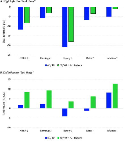
Figure 5, panel A summarizes the results of the high-inflation bad times presented in Table 4. Clearly, for the multi-asset investor stagflationary and other bad times episodes are challenging, while the same asset allocation including factor premiums perform better in each of these sub-regimes. Figure 5, Panel B summarizes the results during deflationary bad times. Although returns on traditional portfolios are substantially better than during high-inflation bad times, deflationary bear markets also present a challenge for investors. Again, factor premiums consistently improve on traditional portfolios. Overall, we can conclude that the most severe bad times for investors in traditional asset classes are times of high inflation with either economic or earnings downturns, rising rates, falling equity markets, rising inflation, or deflationary bear markets, and factor premiums on average help to alleviate the pain during these periods.

Figure 5. Stagflationary Times and Investment Returns, 1875–2021

Notes: The figure shows the historical average return on (i) the 60/40 global equity/bond portfolio and (ii) the 60/40 portfolio augmented with equity, bond, and global factor premiums across high-inflation “bad time” regimes (panel A) or deflationary bad times (panel B). High-inflation (deflationary) times and defined as high- (>4%; low, <0%) inflation periods in combination with an economic recession (National Bureau of Economic Research [NBER]), falling corporate earnings, falling equities, rising rates, or inflation (changes over a 12-month period). The sample period is 1875 to 2021.

Concluding Remarks

We examine investment returns across inflationary regimes. As more extreme inflation regimes—like high inflation, stagflation, and deflation—are relatively uncommon, we utilize a deep sample between 1875 and 2021. Inflation has varied considerably over time, fluctuating between deflationary, moderate-inflation, or high-inflation (including stagflationary) regimes. Moreover, inflation has generally been an important topic for investors over the past 147 years. Asset class and factor premiums are strong and consistent “empirical facts,” with attractive significant average returns over time. However, asset class premiums vary substantially across inflationary regimes. Deflationary and moderate inflation scenarios generally provide positive nominal and real equity and bond returns, while real returns especially suffer during times of high inflation. Splitting up inflationary regimes into sub-regimes reveals that stagflationary episodes, inflationary bear markets, or rising inflationary times and, to a lesser extent, deflationary bear markets are bad times for investors. During these “bad times,” multi-factor equity, multi-factor bond, and GFPs are consistent and attractive as they are across inflationary regimes. Such factors help to alleviate the pain during bad times, offsetting some of the negative impact of high inflation.

These results have several important implications. First, for investors, times of high inflation, and especially stagflation and inflationary bear markets, are challenging, which suggests that long-term asset class premiums may be a compensation for bearing risks during these bad times. Second, as equity, bond, and GFPs are generally consistent across inflationary regimes, they provide diversification to traditional asset class investments. Still, these factor premiums do not take away inflation risk, as their returns do not substantially increase during bad times. Third, our results suggest that factor premiums in equities and bonds and across asset classes are not a compensation for bearing inflationary risks. Finally, our results indicate that portfolio managers may be better off with a balanced exposure to multiple factor premiums instead of trying to dynamically rotate across factors based on inflation.

Acknowledgments

We would like to thank Campbell Harvey, David Blitz, Martin Martens, and Olaf Penninga for valuable contributions and discussions. The views expressed in this paper are not necessarily shared by Robeco Institutional Asset Management.

Disclosure Statement

The authors are employed by Robeco, a firm that offers various investment products. The construction of these products may, at times, draw on insights related to this research. That said, the research article is independent of the views of Robeco and solely attributable to the authors.

Additional information

Notes on contributors

Guido Baltussen

Guido Baltussen is a professor at Erasmus University Rotterdam, and head of factor investing and co-head of quant fixed income at Robeco Institutional Asset Management, Rotterdam, the Netherlands.

Laurens Swinkels

Laurens Swinkels is an associate professor at Erasmus University Rotterdam, and head of quant strategy for sustainable multi asset solutions at Robeco Institutional Asset Management, Rotterdam, the Netherlands.

Bart van Vliet

Bart van Vliet, CFA, is a PhD candidate at Erasmus University Rotterdam, and manager of client reporting at Robeco Institutional Asset Management, Rotterdam, the Netherlands.

Pim van Vliet

Pim van Vliet is head of conservative equities and chief quant strategist at Robeco Institutional Asset Management, Rotterdam, the Netherlands.

Notes

1 Several authors have examined the inflation-hedging characteristics of a variety of asset classes over different investment horizons; see, for example, Froot (1995), Schotman and Schweitzer (2000), Martin (2010), Crawford, Liew, and Marks (2013), and Podkaminer, Tollette, and Siegel (2022). These studies typically focus on the United States instead of global markets and examine considerably shorter sample periods than we do.

2 For equity factors, we use the dataset on U.S. equity factors compiled by Baltussen, Van Vliet, and Van Vliet (2022), combined with data from Wahal (2019). For bond market factors, we use data from Baltussen, Martens, and Penninga (2021) on global government bond factor premiums. For global (“cross-asset”) factor premium, we use the dataset compiled by Baltussen, Swinkels, and Van Vliet (2021).

3 More specifically, Neville et al. (2021) roughly define inflationary times as those periods when year-over-year realized inflation rises above 5% or has not fallen back below 50% of its peak over a rolling 24-month window.

4 We choose to focus on CPI as core measure of inflation instead of GDP deflators, as the former measures inflation average prices of the typical expenditure basket of an urban consumer and is typically considered as the headline number by investors, while GDP deflators focus on average prices of domestically produced final goods and services within an economy.

5 Barsky and De Long (1991) investigate U.S. inflation expectations in the period before World War I and conclude that they may have been related to increased gold production.

6 See, for example, The Guardian (24 June 2021) “Recovery likely to push inflation above 3% by end of year, says Bank”.

7 More specifically, we employ a bag of words approach by counting the relative frequency of words each day related to inflation (including inflation, inflationary, and stagflation) and deflation (i.e., including deflation, deflationary, disinflation, anti-inflationary, and noninflationary), see Garcia (2013) for more specifics about the bag of words approach and information about The New York Times columns. We utilize the approach of Garcia (2013) but apply it to inflation or deflation by taking all inflation-related words in the TIAA-CREF financial glossary and the General Inquirer dictionary. Further, in line with an annual inflation horizon, we compute an annual average and compute its rolling 10-year standardized Z score. We assign a resulting value of 1 (–1) when the Z score exceeds 1 (falls below –1).

8 We do not include the size factor. Baltussen, Van Vliet, and Van Vliet (2022) show that there is no long-run evidence for an alpha relative to the capital asset pricing model in the United States, confirming the observation of Blitz and Hanauer (2020) that size is a weak stand-alone factor in international equity markets. In (unreported) robustness results, we have verified that conclusions on size across inflationary regimes are not materially different from other equity factors.

9 The time-series we use are updated versions of the data that have been made available online at https://doi.org/10.25397/eur.14237024.v1. We do not include cross-sectional Momentum, as its returns are highly correlated with those of time-series Momentum (also known as Trend). We also do not include the monthly seasonal factor, which is difficult to line up with our annual inflation measure.

10 Equities and bonds have historically been the most important asset classes making up the invested market portfolio; see Doeswijk, Lam, and Swinkels (2020). For example, commodities make up less than 2.5% of the market portfolio over the period 1960 to 2017. In this study, we do not include corporate bonds as a good historical database on the returns of investing in corporate bonds going back to 1875 is to the best of our knowledge not available.

11 This is fairly similar to the arithmetic (geometric) average of 10.65% (8.45%) reported in Jordá et al. (2019) over the period 1870 to 2015.

12 Jordá et al. (2019) report an arithmetic (geometric) 6.06% (5.71%) return for government bonds and a 4.58% (4.53%) return for cash over the period 1870 to 2015.

13 Relatedly, Garbade (2008) explains that from 1920 onward, Treasury certificates had been brought to the market for a fixed price. This resulted in massive oversubscriptions because the fixed issue price was lower than their market value after issuance. Snowden (1990) argues that it seems more important to include a short-term instrument that carries some default risk rather than not using one at all. Moreover, it is not the case that data on default-free securities are not available, but rather that commercial paper was the closest to default-free present in financial markets. Siegel (1992) attempts to remove this default premium from U.S. commercial paper rates by using the term structure observed in the United Kingdom, which was more likely the global risk-free rate of the time; see Friedman and Schwartz (1982). Similar issues may also be at play for the other government bond markets outside the United States in our sample, leading to term premia that are lower than we have observed in more recent markets where an entire term-structure of (near) default-free government securities can be traded.

14 Also see, for example, Asness, Moskowitz, and Pedersen (2013) for evidence that a combination of Value and Momentum is significant.

15 As discussed in Baltussen, Swinkels, and Van Vliet (2021), the Low Risk factor works better within asset classes than across markets, which is confirmed by the fact that Low Risk is the strongest factor in equities (panel B) and the second strongest in bonds (panel C), but the weakest factor in global markets (panel D).

16 Note that Cohen, Polk, and Vuolteenaho (2005) find that the risk-return relation becomes inverse during inflationary times, indicating a larger Low Risk premium in equities. By contrast, Neville et al. (2021) find that Betting-Against-Beta (BAB) is significantly weaker during times of inflation. With this extended series based 2 × 3 sorted portfolios with value weighting (which prevent an extreme size bias or large exposure to illiquid stocks), we do not find a clear relation between Low Risk equities and inflation.

17 We proxy a long-only investment with a 100% allocation to the market and a 50% allocation to the long-short multi-factor premium strategy in that asset class.

18 Extending the horizon to 5 years still gives negative real equity returns.

19 Factor timing involves additional risk and additional transaction costs. Besides inflation, one could consider factor value spreads (Cohen, Polk, Vuolteenaho, 2003), factor momentum (Ehsani and Linnainmaa 2022), and other macro indicators if the aim is to improve the multi-factor mix.

20 See https://www.nber.org/research/data/us-business-cycle-expansions-and-contractions.

21 We have verified that results are similar when using the Global Recession Indicator from the OECD when available (and before availability backfilled with NBER data), which dates back to the 1960s, motivating our choice of NBER dates. Historical business cycle dating exercises for other countries stretching back to the 19th century are not readily available. As alternative we have also evaluated the sign of the annual changes in nominal GDP across the United States, United Kingdom, Germany, France, and Japan, finding again similar results (for example the nominal equity return (60/40) during stagflationary episodes equals –14.9% (–8.9%), and factors materially improve this number).

22 https://www.nber.org/research/data/us-business-cycle-expansions-and-contractions.

23 http://www.econ.yale.edu/∼shiller/data.htm.

24 In this study, we choose to not include other asset classes like aggregate returns on global real estate, commodities, or credit markets due to a lack of index data in the beginning of our sample. Commodities futures data are available as of 1877 (see Baltussen, Swinkels, and Van Vliet 2021), but only includes agricultural commodities for a large part of our sample, making it in our view less suited as an aggregate commodity market proxy. Further, we do not include Treasury Inflation-Protected Securities (TIPS), assets that are designed to protect the investor against inflation shocks. Investing in them sometimes requires locking in negative real yields, for example since the beginning of 2020 (see Podkaminer, Tollette, and Siegel 2022).

25 Note that we choose to focus on 2 × 3 sorted portfolios to circumvent issues of high tilts to smaller caps and illiquid stocks, as is the case in the Betting-Against-Beta factor in stocks.

Appendix:

Dataset Construction and Robustness Results

A.1 Dataset Construction

In the section below, we describe the data sources and factor definitions used in this study, mostly building upon Baltussen, Van Vliet, and Van Vliet (2022), Baltussen, Martens, and Penninga (2021), and Baltussen, Swinkels, and Van Vliet (2021). For further information, we refer to the studies.

A.1.1 Recession and Earnings Growth Data

We construct our global recession data from the National Bureau of Economic Research (NBER) U.S. recession indicator from the NBER website (1875–2021).²² The corporate earnings data are from the website of Robert Shiller.²³

A.1.2 Asset Class Returns

Equity and bond market returns are sourced from Datastream or Bloomberg, spliced with GFD, as in Baltussen, Swinkels and Van Vliet (2021). We use global equity market returns expressed in USD from MSCI World, and before existence use global value-weighted equity market returns from GFD (ticker TRWLDM) and, in case not available, weighted market returns across key developed markets. For the global government bond returns we use returns on the Bloomberg Barclays Global Treasury index, which we splice inception before with GDP-weighted bond returns across U.S., U.K., German, France, and Japanese bond markets. Bond return data are from Bloomberg and GFD, while GDP data are from the Maddison Project Database (Maddison 2006). All bond returns are hedged to USD, as common in practice as currency risk is a very substantial driver of relative risk in bond portfolios. Cash returns are returns on short-dated U.S. Treasury bills obtained from Kenneth French website and before its inception from Jeremy Siegel.²⁴

A.1.3 Equity Factors

For the pre-1927 data, we use data from Baltussen, Van Vliet, and Van Vliet (2022); for the post-1926 data, we use the Kenneth French online data library. Baltussen, Van Vliet, and Van Vliet (2022) have compiled their data from several sources in order to obtain a reliable and historically extensive dataset. The sample covers 61 years of data on monthly stock prices, dividend yields, and market capitalizations for all major stocks traded on the NYSE, NY Curb, and regional exchanges. The sample spans the period from January 1866 through December 1926 and is at the monthly frequency. They build their dataset from the Commercial and Financial Chronicle (CFC, which was also used to build the CRSP sample as of 1926) and Global Financial Data (GFD). Note that we use their series from 1875 until 1926.

The equity factors are constructed as follows:

• Value:

  • 1875–1926: Dividend yield. Source: Baltussen, Van Vliet, and Van Vliet (2022).

  • 1927–2021: Book-to-market (HML). Source. Kenneth French on-line data library.

• Momentum:

  • 1875–1926: Past 12-1 month total return. Source: Baltussen, Van Vliet, and Van Vliet (2022).

  • 1927–2021: Past 12-1 month total return (MOM). Source. Kenneth French on-line data library.

• Low risk:

  • 1875–1926: Past 36-month beta. Beta neutral long-short portfolio. Source: Source: Baltussen, Van Vliet, and Van Vliet (2022).

  • 1927–2021: Past 36-month volatility. Volatility neutral long-short portfolio.²⁵ Source. www.paradoxinvestor.com.

• Quality (50% Profitability & 50% Investment):

  • 1875–1939: Not available, because companies did not have (standardized) accounting data, see Wahal (2019) and Baltussen, Van Vliet, and Van Vliet (2022).

  • 1940–1962: Operating profitability, defined as revenues minus cost of goods sold, minus selling, general, and administrative expenses, minus interest expense, scaled by book equity. Investments, defined as the change in total assets from the fiscal year ending in year t-2 to the fiscal year ending in t-1, divided by t-2 total assets. Source: Wahal (2019).

  • 1963–2021: Operating profitability (RMW) and Investments (CMA), defined the same as above. Source. Kenneth French on-line data library.

A.1.4 Bond Factors

For bond market factors, we use data from Baltussen, Martens, and Penninga (2021) on global government bond factor premiums. They have compiled data from 31 December 1799 through 31 December 2020, which in this paper we extend by 1 year. The paper sources bond futures prices and return data from Bloomberg and splice these with bond index-level data from Datastream, backfilled before inception with Global Financial Data (GFD). From the same sources, they obtain yields and inflation data, the latter extended where possible with data from Macrohistory.net. They apply a 2-month lag to inflation numbers to mimic their real-time availability.

• Value: Real yield (bond yield minus inflation). Available 1875–2021.

• Momentum: Past 12-1 month total return. Available 1875–2021.

• Low Risk: 36-month beta. Beta neutral long-short portfolio on the U.S. bond curve. Available 1922–2021.

• Carry: Term spread (bond yield minus short-term interest rate). Available 1875–2021.

A.1.5 Global Factor Premiums

For global (“cross-asset”) factor premium, we use the dataset and definitions from Baltussen, Swinkels, and Van Vliet (2021). They source price and return data of equity futures and indices from Bloomberg, Datastream, and Global Financial Data. Their primary source is the futures from Bloomberg, with gaps filled in by Datastream data and spliced before futures inception with index-level data, as in Baltussen et al. (2019). They backfill these data with equity index–level data downloaded from Global Financial Data and obtain dividend yields from the same sources. For Carry, they use the spot, front futures, and second futures prices. Before they have data on futures, they reconstruct the monthly implied carry as if these markets had listed futures using the regression methodology on the difference between total return and price indices. The markets considered are spread around the globe and cover the major developed markets with substantial data history.

Bond futures price and return data are sourced from Bloomberg and splice these with bond index–level data from Datastream, backfilled before inception with Global Financial Data. From the same sources, they obtain yields and inflation data, the latter extended when possible with data from Macrohistory.net. The markets considered are the major developed bond markets around the globe.

Currency forward and spot prices are primarily from Datastream, spliced with Bloomberg data and Global Financial Data. Purchasing power parity data are obtained from the OECD website and, before 1971, with data from Macrohistory.net. The main measure for the financing rates is short-term London Inter-bank Offered Rate (LIBOR) rates (sourced from Bloomberg and Datastream), spliced with (in order of usage) Eurodollar rates from Datastream, short-term Treasury bill rates and commercial paper yields from Global Financial Data, and short rates from Macrohistory.net and, for the United States, with data from Jeremy Siegel. When all are unavailable, they splice with lagged Treasury bill returns.

Commodity futures price and return data are sourced from Bloomberg, spliced with monthly commodity futures data from CBOT annual reports (1877–1962) obtained from TwoCenturies.com. For the commodity Value measure, they use commodity spot prices from Bloomberg and Datastream, spliced with spot data from Global Financial Data and TwoCenturies.com. For Carry, they use the front futures and second futures prices. The main contracts based on their general usage and liquidity are included. Due to restrictions on tradability, they exclude gold as a speculative asset during the currency gold standard up to the end of the Bretton Woods system (which was effectively a gold standard) in 1971.

The factors in their dataset are constructed as follows:

• Value: For equities, the dividend-to-price ratio (D/P) defined as past 12-month dividend payment by the current price, for government bonds the Real yield (bond yield minus inflation), for currencies an equally weighted combination of absolute and relative purchasing power parity, and for commodities, the 5-year reversal in spot prices.

• Momentum/Trend: Time-series Momentum that takes a long (short) position if the 12-1 month return is positive (negative).

• Low Risk: Past 36-month beta with respect to asset class. Beta neutral long-short portfolio.

• Carry: For equities the excess implied dividend yield priced into the futures versus spot contract, for government bonds the slope of the yield curve defined as the 10-year yield minus the short rate, for currencies the short-term yield differential, and for commodities the slope of the futures curve.

A.2 Robustness Results

 

Table A1. Robustness Results: Inflation Classifications

A. Global equity, bond, and cash returns
				Nominal Returns				Real Returns
Inflation Bucket	N (ann.)	Inflation (avg.)	Equities	Bonds	Cash	60/40	Equities	Bonds	Cash	60/40
<3%	87.7	0.4	9.0	4.7	2.9	7.3	8.6	4.3	2.5	6.9
>3%	59.3	7.4	7.4	4.2	4.1	6.1	0.0	–3.2	–3.3	–1.3
Wald	–	–	0.5	0.4	8.4**	0.6	11.0**	46.4**	58.5**	20.1**
<5%	113.3	1.2	9.3	4.9	3.2	7.5	8.1	3.7	2.0	6.3
>5%	33.8	10.1	5.4	3.1	4.0	4.5	–4.6	–6.9	–6.1	–5.5
Wald	–	–	1.3	4.4**	1.7	2.0	11.6**	62.3**	70.3**	21.0**
All	147	3.2	8.4	4.5	3.4	6.8	5.1	1.2	0.1	3.6
B. Factors returns
	Inflation Bucket	<3%	>3%	Wald		<5%	>5%	Wald
Equity factors	Value	3.0	4.2	0.5		3.0	5.2	1.1
	Momentum	6.3	7.8	0.7		6.6	7.9	0.5
	Low Risk	6.8	6.0	0.2		7.4	3.4	5.1**
	Quality	3.0	1.9	1.1		2.9	1.4	2.9
	MFE	5.1	5.1	0.0		5.3	4.6	0.6
Bond factors	Value	1.2	4.3	4.9**		2.0	4.0	1.3
	Momentum	5.3	1.8	5.1**		5.1	0.0	8.0**
	Low Risk	3.2	5.8	1.8		3.8	6.2	1.6
	Carry	7.6	7.1	0.1		7.5	7.0	0.1
	MFB	4.6	4.5	0.0		4.8	3.8	0.9
Global factors	Value	2.4	2.1	0.2		2.3	2.2	0.0
	Mom (Trend)	6.9	8.0	1.1		6.9	8.9	2.2
	Low Risk	1.3	2.0	1.1		1.6	1.4	0.1
	Carry	5.8	5.2	0.4		6.0	3.9	3.7
	GFP	4.1	4.3	0.0		4.2	4.1	0.5

Notes: The table shows historical returns on asset classes (panel A), and equity, bond, and global macro factor premiums (panel B) bucketed by two different global inflation category definitions (<3% vs. >3% and <5% vs. >5%). The sample period is 1875 to 2021. Returns are in percentages per annum. Significance at the 5% significance level is denoted with * and significance at the 1% significance level with **. A Wald F test is used to test for significant average return differences across the different inflationary states. All standard errors are computed using the Newey–West procedure.

Table A2. Robustness Results: Annual Changes in Inflation

A. Global equity, bond, and cash returns
				Nominal Returns				Real Returns
Change in Infl. Bucket	N (ann.)	Inflation (avg.)	Equities	Bonds	Cash	60/40	Equities	Bonds	Cash	60/40
<0%	74.9	–2.5	7.7	5.5	5.2	6.8	10.2	8.0	7.8	9.3
0–2%	44.9	0.8	10.0	4.2	3.3	7.7	9.2	3.4	2.5	6.9
2–4%	10.7	2.9	7.5	2.7	2.7	5.6	4.7	–0.2	–0.2	2.7
>4%	16.5	7.4	7.7	1.6	5.9	5.3	0.3	–5.8	–1.5	–2.2
All	147.0	3.2	8.4	4.5	3.4	6.8	5.1	1.2	0.1	3.6
Wald	–	–	1.1	8.1**	0.9	1.2	2.9*	55.7**	51.3**	8.3**
B. Factors returns
	Change in Infl. Bucket	<0%	0%–2%	2%–4%	>4%	All	Wald
Equity factors	Value	3.4	2.9	4.0	5.1	3.5	0.2
	Momentum	9.0	4.4	0.0	8.5	6.9	3.3*
	Low risk	8.3	4.3	5.5	4.8	6.5	2.7*
	Quality	2.7	2.4	2.3	1.2	2.5	0.5
	MFE	6.4	3.4	2.8	5.7	5.1	3.8*
Bond factors	Value	3.9	1.9	–1.8	–0.3	2.4	3.6*
	Momentum	4.2	4.4	3.7	1.0	3.9	0.8
	Low risk	7.4	6.6	8.6	8.7	7.4	1.4
	Carry	4.6	3.6	8.9	2.8	4.4	0.6
	MFB	5.1	4.2	4.5	3.3	4.6	1.3
Global factors	Value	3.3	2.3	–1.4	0.2	2.3	6.7**
	Mom (Trend)	7.2	6.7	8.3	9.5	7.4	1.5
	Low risk	1.3	2.0	1.7	1.5	1.6	0.6
	Carry	5.4	6.6	4.4	4.2	5.5	2.2
	GFP	4.3	4.4	3.2	3.8	4.2	2.0

Notes: The table shows historical returns on asset classes (panel A) and equity, bond, and global macro factor premiums (panel B) bucketed by four global inflation categories (from deflation, <0%, to high inflation, >4%) using annual changes in inflation. The sample period is 1875 to 2021. Returns are in percentages per annum. Significance at the 5% significance level is denoted with * and significance at the 1% significance level with **. A Wald F test is used to test for significant average return differences across the different inflationary states. All standard errors are computed using the Newey–West procedure.

Table A3. Robustness Results: U.S. Inflation Analysis

A. Global equity, bond, and cash returns
				Nominal Returns				Real Returns
Inflation Bucket	N (ann.)	Inflation (avg.)	Equities	Bonds	Cash	60/40	Equities	Bonds	Cash	60/40
<0%	27.6	–3.6	5.2	5.2	4.1	5.2	8.8	8.8	7.7	8.8
0%–2%	42.0	1.0	8.9	3.9	3.9	6.9	7.9	2.9	2.9	5.9
2%–4%	40.3	2.9	10.1	5.4	5.2	8.2	7.2	2.5	2.3	5.3
>4%	37.2	7.9	8.2	3.6	4.8	6.4	0.4	–4.3	–3.1	–1.5
All	147.0	3.2	8.4	4.5	3.4	6.8	5.1	1.2	0.1	3.6
Wald	–	–	0.9	3.0*	7.9**	1.0	2.0	30.7**	37.7**	5.5**
B. Factors returns
	Inflation Bucket	<0%	0–2%	2–4%	>4%	All	Wald
Equity factors	Value	4.1	1.5	3.3	5.5	3.5	1.2
	Momentum	4.3	5.9	8.5	8.3	6.9	1.2
	Low Risk	6.9	8.2	6.9	3.9	6.5	1.9
	Quality	2.4	2.0	2.8	2.5	2.5	0.2
	MFE	5.3	4.6	5.6	5.2	5.1	0.3
Bond factors	Value	0.9	2.5	1.1	5.0	2.4	2.1
	Momentum	5.8	5.7	2.9	1.6	3.9	2.0
	Low Risk	4.2	3.6	3.4	6.5	4.4	0.8
	Carry	7.5	8.2	6.8	7.0	7.4	0.3
	MFB	4.7	5.3	3.6	4.8	4.6	1.5
Global factors	Value	1.2	2.9	2.5	2.1	2.3	1.0
	Mom (Trend)	7.9	6.1	6.8	9.0	7.4	2.1
	Low Risk	0.5	1.0	1.9	2.7	1.6	2.0
	Carry	4.2	5.8	6.1	5.5	5.5	1.0
	GFP	3.5	4.0	4.3	4.8	4.2	2.4

Notes: The table shows historical returns on asset classes (panel A), and equity, bond, and global macro factor premiums (panel B) bucketed by four inflation categories (from deflation, <0%, to high inflation, >4%) using U.S. inflation data only. The sample period is 1875 to 2021. Returns are in percentages per annum. Significance at the 5% significance level is denoted with * and significance at the 1% significance level with **. A Wald F test is used to test for significant average return differences across the different inflationary states. All standard errors are computed using the Newey–West procedure.

Table A4. Robustness Results: Subsamples 1875 to 1948 and 1949 to 2021

A. 1875–1948
				Nominal Returns				Real Returns
Inflation Bucket	N (ann.)	Inflation (avg.)	Equities	Bonds	Cash	60/40	Equities	Bonds	Cash	60/40
<0%	21.3	–3.3	2.9	5.4	3.0	3.9	6.2	8.7	6.3	7.2
0%–2%	17.3	1.0	8.2	3.3	3.3	6.3	7.2	2.4	2.4	5.3
2%–4%	12.2	2.8	8.6	3.0	3.2	6.4	5.8	0.2	0.4	3.6
>4%	23.3	10.0	2.5	1.7	2.1	2.2	–7.5	–8.2	–7.9	–7.8
All	74.0	3.2	4.9	3.4	2.8	4.3	1.7	0.1	–0.4	1.1
Wald	–	–	2.0	4.8**	4.8**	1.4	3.2*	32.9**	60.4**	6.0**
	Inflation Bucket	<0%	0–2%	2–4%	>4%	All	Wald
Equity factors	Value	5.3	4.1	1.2	3.5	3.8	0.5
	Momentum	7.6	5.0	4.6	4.9	5.6	0.1
	Low Risk	8.0	5.7	4.0	5.5	6.0	0.5
	Quality	–	–	2.9	–0.8	–0.7	–
	MFE	5.3	4.1	1.2	3.5	3.8	0.8
Bond factors	Value	0.1	2.4	–2.2	2.2	0.9	0.8
	Momentum	6.4	7.9	8.6	0.4	5.2	2.7*
	Low Risk	11.2	3.6	0.9	1.4	4.6	3.2*
	Carry	8.1	9.6	10.7	1.8	6.9	4.3**
	MFB	5.5	6.7	5.7	1.4	1.4	5.9**
Global factors	Value	0.9	3.3	0.6	2.4	1.9	1.8
	Mom (Trend)	7.5	7.6	7.5	7.6	7.5	0.0
	Low Risk	1.1	0.7	0.5	1.3	1.0	0.4
	Carry	4.8	6.7	7.5	1.5	4.6	6.5**
	GFP	3.6	4.6	4.0	3.2	3.8	2.1
B. 1949–2021
				Nominal Returns				Real Returns
Inflation Bucket	N (ann.)	Inflation (avg.)	Equities	Bonds	Cash	60/40	Equities	Bonds	Cash	60/40
<0%	1.8	–0.9	–	–	–	–	–	–	–	–
0%–2%	25.7	1.4	13.0	5.5	2.4	10	11.5	4.1	0.9	8.6
2%–4%	22.8	2.8	12.3	5.3	3.5	9.5	9.4	2.4	0.6	6.6
>4%	22.8	7.1	11.4	6.2	6.4	9.3	4.3	–0.9	–0.7	2.2
All	73.0	3.2	11.9	5.6	3.9	9.4	8.6	2.4	0.7	6.1
Wald	–	–	1.7	0.6	19.4**	2.3	2.1	4.2	0.5	2.9*
	Inflation Bucket	<0%	0–2%	2–4%	>4%	All	Wald
Equity factors	Value	–	2.2	3.1	5.4	3.2	3.1*
	Momentum	–	6.8	9.0	10.7	8.2	1.7
	Low Risk	–	8.6	6.1	7.0	7.0	1.3
	Quality	–	3.3	2.2	3.0	2.9	0.8
	MFE	–	5.2	5.1	6.5	5.3	2.7*
Bond factors	Value	–	1.7	2.6	7.4	3.9	2.4
	Momentum	–	3.0	4.6	0.5	2.6	1.8
	Low Risk	–	2.1	3.3	7.7	4.3	1.6
	Carry	–	6.3	7.3	10.5	7.8	1.3
	MFB	–	3.3	4.4	6.5	4.6	2.4
Global factors	Value	–	3.2	2.6	1.9	2.6	0.4
	Mom (Trend)	–	7.4	4.8	10.2	7.2	9.9**
	Low Risk	–	1.3	3.0	2.7	2.2	6.2**
	Carry	–	5.5	6.9	7.3	6.5	0.8
	GFP	–	4.4	4.3	5.5	4.6	2.8*

Notes: The table shows historical returns on asset classes, equity, bond, and global macro factor premiums bucketed by four global inflation categories (from deflation, <0%, to high inflation, >4%). Panel A includes the first sample period 1875 to 1948, and panel B includes the second sample period 1949 to 2021. Returns are in percentages per annum. Significance at the 5% significance level is denoted with * and significance at the 1% significance level with **. A Wald F test is used to test for significant average return differences across the different inflationary states. All standard errors are computed using the Newey–West procedure.

References

- Asness, C. S., T. J. Moskowitz, and L. H. Pedersen. 2013. “Value and Momentum Everywhere.” The Journal of Finance 68 (3): 929–85. doi:10.1111/jofi.12021.
- Baltussen, Guido, Martin Martens, and Olaf Penninga. 2021. “Factor Investing in Sovereign Bond Markets: Deep Sample Evidence.” The Journal of Portfolio Management 48 (2): 209–25. doi:10.3905/jpm.2021.1.311.
- Baltussen, G., L. Swinkels, and P. Van Vliet. 2021. “Global Factor Premiums.” Journal of Financial Economics 142 (3): 1128–54. doi:10.1016/j.jfineco.2021.06.030.
- Baltussen, G., S. Van Bekkum, and Z. Da. 2019. “Indexing and Stock Market Serial Dependence around the World.” Journal of Financial Economics 132 (1): 26–48. doi:10.1016/j.jfineco.2018.07.016.
- Baltussen, G., B. Van Vliet, and P. Van Vliet. 2022. “The Cross-Section of Stock Returns before 1926 (and beyond).” SSRN Working Paper 3969743.
- Barsky, R., and B. De Long. 1991. “Forecasting pre-World War I Inflation: The Fisher Effect and the Gold Standard.” The Quarterly Journal of Economics 106 (3): 815–36. doi:10.2307/2937928.
- Blitz, D. 2021. “The Quant Cycle.” The Journal of Portfolio Management 48 (2): 26–43. doi:10.3905/jpm.2021.1.304.
- Blitz, D., and M. Hanauer. 2020. “Settling the Size Matter.” The Journal of Portfolio Management 47 (2): 99–112. doi:10.3905/jpm.2020.1.187.
- Cagan, P. 1956. “The Monetary Dynamics of Hyperinflation.” In: Studies in the Quantity Theory of Money, edited by M. Friedman, 25–117. Chicago, IL: University of Chicago Press.
- Cohen, R., C. Polk, and T. Vuolteenaho. 2003. “The Value Spread.” The Journal of Finance 58 (2): 609–41. doi:10.1111/1540-6261.00539.
- Cohen, R., C. Polk, and T. Vuolteenaho. 2005. “Money Illusion in the Stock Market: The Modigliani-Cohn Hypothesis.” Quarterly Journal of Economics 120 (2): 639–68. doi:10.1162/0033553053970133.
- Crawford, G., J. Liew, and A. Marks. 2013. “Investing under Inflation Risk.” The Journal of Portfolio Management 39 (3): 123–35. doi:10.3905/jpm.2013.39.3.123.
- Doeswijk, R., T. Lam, and L. Swinkels. 2020. “Historical Returns of the Market Portfolio.” The Review of Asset Pricing Studies 10 (3): 521–67. doi:10.1093/rapstu/raz010.
- Ehsani, S., and J. Linnainmaa. 2022. “Factor Momentum and the Momentum Factor.” The Journal of Finance 77 (3): 1877–919. doi:10.1111/jofi.13131.
- Ely, D., and K. Robinson. 1997. “Are Stocks a Hedge against Inflation? International Evidence Using a Long-Run Approach.” Journal of International Money and Finance 16 (1): 141–67. doi:10.1016/S0261-5606(96)00039-3.
- Friedman, M., and A. Schwartz. 1982. Monetary Trends in the United States and the United Kingdom. Chicago, IL: University of Chicago Press.
- Froot, K. 1995. “Hedging Portfolios with Real Assets.” The Journal of Portfolio Management 21 (4): 60–77. doi:10.3905/jpm.1995.409527.
- Garbade, K. 2008. “Why the U.S. Treasury Began Auctioning Treasury Bills in 1920.” Federal Reserve Bank of New York Economic Policy Review, 14.
- Garcia, D. 2013. “Sentiment during Recessions.” The Journal of Finance 68 (3): 1267–300. doi:10.1111/jofi.12027.
- Ilmanen, A., and J. Kizer. 2012. “The Death of Diversification Has Been Greatly Exaggerated.” The Journal of Portfolio Management 38 (3): 15–27. doi:10.3905/jpm.2012.38.3.015.
- Jordá, O., K. Knoll, D. Kuvshinov, M. Schularick, and A. Taylor. 2019. “The Rate of Return on Everything, 1870–2015.” The Quarterly Journal of Economics 134 (3): 1225–98. doi:10.1093/qje/qjz012.
- Maddison, A. 2006. The World Economy, A Millennial Perspective. Paris: OECD Publishing.
- Martin, G. 2010. “The Long-Horizon Benefits of Traditional and New Real Assets in the Institutional Portfolio.” The Journal of Alternative Investments 13 (1): 6–29. doi:10.3905/jai.2010.13.1.006.
- Neville, H., T. Draaisma, B. Funnell, C. Harvey, and O. Van Hemert. 2021. “The Best Strategies for Inflationary Times.” The Journal of Portfolio Management 47 (8): 8–37. doi:10.3905/jpm.2021.1.274.
- Podkaminer, E., W. Tollette, and L. Siegel. 2022. “Protecting Portfolios against Inflation.” Journal of Investing 31 (3): 23–44. doi:10.3905/joi.2021.1.207.
- Schotman, P., and M. Schweitzer. 2000. “Horizon Sensitivity of the Inflation Hedge of Stocks.” Journal of Empirical Finance 7 (3-4): 301–15. doi:10.1016/S0927-5398(00)00013-X.
- Siegel, J. 1992. “The Real Rate of Interest from 1800 to 1900: A Study of the U.S. and U.” Journal of Monetary Economics, 29 (2): 227–52. doi:10.1016/0304-3932(92)90014-S.
- Snowden, K. 1990. “Historical Returns and Security Market Development, 1872–1925.” Explorations in Economic History 27 (4): 381–420. doi:10.1016/0014-4983(90)90022-Q.
- Svensson, L. 2011. “Inflation Targeting.” In Handbook of Monetary Economics, edited by M. Friedman and M. Woodford, Volume 3b, 1237–302. Amsterdam, Netherlands: Elsevier.
- Wahal, S. 2019. “The Profitability and Investment Premium: Pre-1963 Evidence.” Journal of Financial Economics 131 (2): 362–77. doi:10.1016/j.jfineco.2018.09.007.