Conservative finite-difference scheme for the 2D problem of femtosecond laser pulse interaction with kink structure of high absorption in semiconductor

ABSTRACT

The problem of high-intense laser pulse interaction with a semiconductor under the condition of a light energy nonlinear absorption, which results in high absorption domains formation, is considered. Such interaction allows reaching a construction of an element for all-optical data treatment. For its adequate description we propose new mathematical model taking into account the longitudinal and transverse diffraction effects. The longitudinal diffraction induced a reflection of laser radiation from boundaries of the high absorption domains that results in changing of their spatial structure. The conservative finite-difference scheme (FDS) is developed for numerical computation of the complicated nonlinear processes. The property of the FDS conservatism is proved. For the proposed FDS realization the two-stage iteration method is proposed. Computer simulation results are presented. We show the uniform boundedness of the mesh functions at the iterations and the convergence of the iteration process. We show also positiveness and boundedness of the mesh function corresponding to free-charged particles. We discuss some properties of differential problem including the problem invariants, positiveness of the free-charged concentrations.

KEYWORDS:

• Conservative finite-difference scheme
• femtosecond laser pulse
• nonlinear absorption
• diffraction of laser beam
• kink structure

2010 MSC CLASSIFICATIONS:

• 65N06
• 65N12
• 35Q60

1. Introduction

Laser radiation interaction with a semiconductor is a very modern problem for the past decade. One of the important application of such investigation is a creation of an optical bistable element using various nonlinear responses of a semiconductor at a laser radiation exposure. As it is well-known, the optical bistability (OB) is a very promising phenomenon for creation and developing of all-optical data processing and many authors pay their attention to OB phenomenon research since pioneer works [10,11] and continued, for example, in [8,9,13,15,19,23,28,31,32,33,38,39]. In the case of OB existence, the hysteresis loop of semiconductor characteristics in dependence on a laser pulse intensity takes place. As a result, the domains of charged particles high concentration as well as kink structures of a high absorption could be formed, which results in the appearance of contrast spatial structure of free-charged particle concentration as well as explosive absorption of laser energy. In the present paper, we consider the 2D resonatorless model of the absorption OB.

The femtosecond (${10}^{-15}c$) laser pulse interaction with a semiconductor under the condition of absorption OB occurrence is described by the set of nonlinear PDEs [9]. For numerical solution of such problems, the split-step method is widely used [2,4,6,17,29,30,36,37,40]. For example, in [40] this method is used for a numerical solution of the nonlinear Schrödinger equation. It is shown, how a conservation law and instability are reflected in the numerical finite-difference schemes (FDS). In [37] an efficient time-splitting compact finite-difference method for Gross–Pitaevskii equation is proposed. In [29] a simulation of the nonlinear Schrödinger equation in 1D, 2D and 3D cases is studied on the base of a time-splitting method. The FDS conservatism is investigated on the base of some numerical experiments. In [4] a compact finite-difference method is proposed for the nonlinear Schrödinger equations with constant and variable coefficients.

Much attention is paid to a question of the split-step method properties, such as the conservatism, accuracy and stability. In [2] it is shown, that using of energy-conserving methods for the nonlinear Schrödinger equation, able to conserve a discrete counterpart of the Hamiltonian functional, confers more robustness on the numerical solution of a problem. In [17] the problem of numerical instability of the split-step method applied to the generalized nonlinear Schrödinger equation is widely studied. It should be stressed, that the Fourier method or its modifications applied to such problems [6,40], but this approach requires the certain boundary conditions (BCs) for the problem under consideration. Our aim is to develop the finite-difference method for the problems with arbitrary BCs.

Earlier, at theoretical analysing of the resonatorless OB, in particular in our papers [32,33,34,35] also, the charged particles concentration, a potential of the electric field induced by a laser radiation and a laser pulse intensity changing due to a nonlinear absorption at its propagation in a semiconductor have been considered as a rule. However, it is well-known that the free-charged particle high concentration domains formation is observed under the condition of the hysteresis loop realization. Therefore, a laser beam interaction with these domains may result in partial light reflection from their boundaries. To describe this process, we propose a new mathematical model of the problem. Its main feature consists in a replacement of the equation concerning the laser pulse intensity by the Schrödinger equation with respect to the envelope (complex amplitude, slowly varying in time only) of a wave packet. In our opinion, the diffraction effects could play a significant role for changing the OB element characteristics, such as a stability of the bistable states and time of switching from one state to another one, for example. In this regard, taking into account the diffraction effects at the analysis of switching waves is the urgent problem.

For computer simulation of the problem, we develop a conservative FDS similar to that, which we proposed in [34] for the 2D problem without considering diffraction effects. It is a nonlinear implicit one, so to realize it we proposed an original two-stage iteration process. Computer simulation results confirmed that the FDS also possesses an asymptotic stability property that is very important because we should provide computation during the long time interval.

2. Problem statement

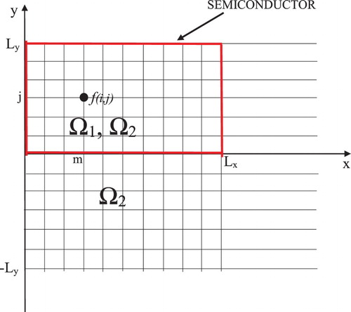
In the present paper, we consider the 2D problem of femtosecond laser pulse interaction with a semiconductor taking into account a longitudinal and transverse diffraction of a laser beam. The semiconductor has a rectangular form and could be placed in the external electric field (Figure 1). Characteristic time of changing the problem parameters is about several tens femtoseconds. A mathematical model for the problem consists from a set of four 2D dimensionless PDEs concerning semiconductor characteristics – free-electron concentration $n\left(x,y,t\right)$, ionized donors concentration $N\left(x,y,t\right)$, electric field potential $\varphi (x,y,t)$ [9,26] and a laser pulse complex amplitude $A\left(x,y,t\right)$, which is slowly varying in time only: (1) $\frac{\mathrm{\partial }N}{\mathrm{\partial }t}=G(n,N,|A{|}^2)-R(n,N),0<x<L_x,0<y<L_y,t>0,$(1) (2) $\frac{\mathrm{\partial }n}{\mathrm{\partial }t}={\kappa }_x\frac{\mathrm{\partial }}{\mathrm{\partial }x}\left(\frac{\mathrm{\partial }n}{\mathrm{\partial }x}-{\mu }_{x}n\frac{\mathrm{\partial }\varphi }{\mathrm{\partial }x}\right)+{\kappa }_y\frac{\mathrm{\partial }}{\mathrm{\partial }y}\left(\frac{\mathrm{\partial }n}{\mathrm{\partial }y}-{\mu }_{y}n\frac{\mathrm{\partial }\varphi }{\mathrm{\partial }y}\right)+G(n,N,|A{|}^2)-R(n,N),$(2) (3) $\frac{{\mathrm{\partial }}^2\varphi }{\mathrm{\partial }{x}^2}+\frac{{\mathrm{\partial }}^2\varphi }{\mathrm{\partial }{y}^2}=\gamma (n-N),$(3) (4) $\frac{\mathrm{\partial }A}{\mathrm{\partial }t}+i{D}_{Ax}\frac{{\mathrm{\partial }}^{2}A}{\mathrm{\partial }{x}^2}+i{D}_{Ay}\frac{{\mathrm{\partial }}^{2}A}{\mathrm{\partial }{y}^2}+\frac{{\beta }_A{\delta }_0}{2}\delta (n,N)A=0,0<x<L_x,-L_y<y<L_y,t>0.$(4)

Figure 1. Setup for computer simulation of the femtosecond pulse interaction with a semiconductor. $E_x$, $E_y$ – external electric field strength (x, y are dimensionless spatial coordinates).

The following notations are used: variables x, y are the dimensionless spatial coordinates, parameters $L_x$, $L_y$ denote their maximal values, correspondingly. Variable t denotes a dimensionless time. The electron diffusion coefficients ${\kappa }_x$, ${\kappa }_y$, the diffraction coefficients $D_{A_x},D_{A_y}$ and the electron mobility coefficients ${\mu }_x$, ${\mu }_y$ are non-negative parameters. Parameter $\gamma$ depends, in particular, on the maximal concentration of free-charged particles. ${\delta }_0$ denotes a maximal value of the semiconductor laser energy absorption. $\chi$ is a wave number, ${\beta }_A=\pi \chi$, $D_{Ay}=1/4\pi \chi$. According to physical sense of the problem, the concentrations $n\left(x,y,t\right)$, $N\left(x,y,t\right)$ and the absorption coefficient $\delta (n,N)$ must be non-negative. Therefore, the concentration $N\left(x,y,t\right)$ must be less or equal to unity, as it is shown in Section 2.1.

The homogenous BCs concerning the free-elector flow correspond to the electric current absence through a semiconductor surface: (5) ${\left.\left(\frac{\mathrm{\partial }n}{\mathrm{\partial }x}-{\mu }_{x}n\frac{\mathrm{\partial }\varphi }{\mathrm{\partial }x}\right)\right|}_{x=0,L_x}={\left.\left(\frac{\mathrm{\partial }n}{\mathrm{\partial }y}-{\mu }_{y}n\frac{\mathrm{\partial }\varphi }{\mathrm{\partial }y}\right)\right|}_{y=0,L_y}=0.$(5) The non-zero electric field strength $E_x$, $E_y$ corresponds to the external electric field presence: (6) ${\left.\frac{\mathrm{\partial }\varphi }{\mathrm{\partial }x}\right|}_{x=0,L_x}=-E_x,{\left.\frac{\mathrm{\partial }\varphi }{\mathrm{\partial }y}\right|}_{y=0,L_y}=-E_y.$(6) We stress that below we consider a case of the external electric field is absent: (7) $E_x=E_y=0.$(7) The zero-value BCs with respect to a complex amplitude correspond to its finite distribution: (8) $A{|}_{x=0,L_x}=A{|}_{y=-L_y,L_y}=0,$(8) and we suppose, that the function A and its nth derivatives on x-coordinate and y-coordinate decrease exponentially when the corresponding coordinate tends to the domain boundaries. Some remarks concerning Equation (4) are discussed in Section 2.4.

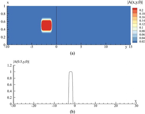
Gaussian beam falls on a semiconductor. We stress that the spatial distribution of a laser pulse complex amplitude along a propagation coordinate coincides with its time distribution because a laser pulse propagates in a linear medium before its interaction with a semiconductor: (9) $\varphi {|}_{t=0}=0,n{|}_{t=0}=N{|}_{t=0}=n_0,A{|}_{t=0}=A_0={\text{e}}^{-{\left(x-L_{xc}\right)}^2/a^2-{\left(y-L_{yc}\right)}^{10}-2i\pi \chi \left(y-L_{yc}\right)},$(9) where $L_{x_c},L_{y_c}$ are coordinates of the incident laser beam centre position, $a$ is a beam radius on x-coordinate. As the initial laser beam profile, which is shown in Figure 2, is a symmetric one, and then the problem solution should also keep symmetry if an external electric field is absent. It is an important feature for numerical method efficiency assessment.

Figure 2. Square root from the intensity distribution of incident pulse (a) and a distribution of square root from the intensity along y-coordinate at beam centre on x-coordinate $(x=L_{xc})$ (b).

Functions G and R describe charged particle’s generation and recombination [9,26] in the area of semiconductor, correspondingly: (10) $G(n,N,|A{|}^2)=q_0|A{|}^2\delta (n,N),$(10) (11) $R(n,N)=\frac{nN-n_0^2}{{\tau }_R},0\le x\le L_x,0\le y\le L_y,t>0$(11) otherwise, these functions are equal to zero: (12) $G(n,N,|A{|}^2)=R(n,N)=0,0\le x\le L_x,-L_y\le y<0,t>0.$(12) We will keep in mind this definition of the functions below. Above $q_0$ is a dimensionless maximum value of the laser pulse intensity, parameter $n_0$ is the equilibrium value of free-electron concentration and ionized donor concentration before the laser pulse action, ${\tau }_R$ characterizes a recombination time (in present work we provide computations for ${\tau }_R=1$). The absorption coefficient $\delta (n,N)$ could be approximated by different ways. Below we consider its following approximation [9]: (13) $\delta (n,N)=(1-N){\text{e}}^{-\psi (1-\xi n)},$(13) where $\xi ,\psi$ are non-negative constants. Boundedness of the absorption coefficient is discussed in Section 2.2. We also write in Section 2.7 some assessments for the electric field potential, which is a solution of Equation (3) and there are some remarks concerning Equation (2) solution existence in Section 2.8.

2.1. Analysis of changing for the function N

Let us prove that the concentration of the ionized donors is less than unity: $N\le 1$. First, we stress that the derivatives from the generation function on the concentrations $n,N$ are: (14) $\frac{\mathrm{\partial }G}{\mathrm{\partial }n}=\xi \psi G\ge 0,\text{if}G\ge 0,$(14) (15) $\frac{\mathrm{\partial }G}{\mathrm{\partial }N}=-{\text{e}}^{-\psi (1-\xi n)}|A{|}^2\le 0.$(15) Consequently, the function G increases with increasing of the concentration n and decreases with increasing of the concentration N.

The corresponding derivatives from the recombination function on the concentrations functions are: (16) $\frac{\mathrm{\partial }R}{\mathrm{\partial }n}=N,\frac{\mathrm{\partial }R}{\mathrm{\partial }N}=n$(16) and this function increases with the concentrations of growth.

At the initial time moment, the functions G and R are equal to zero because the laser intensity is equal to zero and the concentrations are equal to their equilibrium values. If a laser pulse penetrates in a semiconductor then the function G becomes positive and the function N (as well as n) becomes grow. Let us suppose that in certain time moment the function G-R possesses the negative value: the right part of Equation (1) will be negative. Consequently, there is a value $N^{\ast }$(and it is less than unity), at which the right part of Equation (1) is equal to zero. It means that further increase of the function N stops. Thus, the function N cannot be greater than unity.

2.2. Boundedness of the absorption coefficient

Taking into account that the value of the concentration N does not exceed unity, the concentration n is greater than zero, and then the following assessment for the function $\delta (n,N)$ can be written: (17) $\delta (n,N)\le {\delta }_{max}={\text{e}}^{-\psi +\xi \psi n_{max}},n_{max}=\underset{x,y,t}{max}n(x,y,t)$(17) for enough small time interval $t\in [0,t_{\epsilon }]$. More weak assessment can be obtained taking into account the equation [18,22]: (18) $\frac{\mathrm{\partial }}{\mathrm{\partial }t}\left(n+(1-N)\right)=D_x\frac{\mathrm{\partial }{J}_x}{\mathrm{\partial }x}+D_y\frac{\mathrm{\partial }{J}_y}{\mathrm{\partial }y},$(18) where $J_x=\frac{\mathrm{\partial }n}{\mathrm{\partial }x}-{\mu }_{x}n\frac{\mathrm{\partial }\varphi }{\mathrm{\partial }x}\text{,}$ $J_y=\frac{\mathrm{\partial }n}{\mathrm{\partial }y}-{\mu }_{y}n\frac{\mathrm{\partial }\varphi }{\mathrm{\partial }y}$ are the electric current flows.

We see that changing of the concentration sum is due to free-electron flow. Obviously, in small time interval $t\in [0,t_{\epsilon }]$, depending on diffusion coefficients, this flow is close to zero approximately and the derivative on time coordinate in (18) also is equal to zero. In this case, we can believe that the free-electron concentration $n$ is equal to the concentration of ionized donors $N$ (this statement is confirmed by numerical simulation because the diffusion velocity is bounded by the diffusion coefficients and spatial distribution of the free-electron concentration). Therefore, at first stage of laser pulse interaction with a semiconductor (during small time interval) and for qualitative analysis of the absorption coefficient from the free-electron concentration n, we analyse the following function: (19) $\delta (n,N)=\delta \left(n\right)=(1-n){\text{e}}^{-\psi (1-\xi n)}.$(19) To find the maximum of this function we take a first derivative, which is (20) $\frac{\mathrm{\partial }\delta }{\mathrm{\partial }n}=\left(\psi \xi (1-n)-1\right){\text{e}}^{-\psi (1-\xi n)}.$(20) At a value of the concentration $n^{\ast }=1-1/\left(\psi \xi \right),$ the first derivative (20) is equal to zero. The second derivative from the function $\delta \left(n\right)$ is negative at this value of the free-electron concentration (21) $\frac{{\mathrm{\partial }}^2\delta \left(n^{\ast }\right)}{\mathrm{\partial }{n}^2}=-\psi \xi {\text{e}}^{-\psi +\psi \xi -1}<0.$(21) Thus, in a dependence of value for the parameter $\psi \xi$ there are three various dependences of the absorption coefficient from the free-electron concentration, which depicted in Figure 3. We see in Figure 3 if the parameter $\psi \xi$ is greater than unity that there is the same value of the function $\delta \left(n\right)$ for two values of free-electron concentration. It is easy to see that a maximal value of the absorption coefficient is defined by the following formula: (22) ${\delta }_{max}=\left\{\begin{array}{ll}\frac{1}{\psi \xi }{\text{e}}^{-\psi +\psi \xi },& \psi \xi >1,\\ {\text{e}}^{-\psi +\psi \xi },& \psi \xi \le 1.\end{array}\right.$(22)

Figure 3. Qualitative dependence of the absorption coefficient from the free-electron concentration at various values of the parameters multiplication $\psi \xi$.

2.3. Invariants of the problem and some estimation for the problem solution (Equations (1) and (2))

As it is known, the charge conservation law takes place for this problem (23) $Q\left(t\right)={\int }_0^{L_y}{\int }_0^{L_x}\left(n(x,y,t)-N(x,y,t)\right)\text{d}x\text{d}y=\text{const,}$(23) if the charge flow through the semiconductor boundaries is absent. It is easy to see from Equations (1) and (2). To obtain formula (23) it is necessary to subtract Equation (1) from Equation (2) and then to take an integral over the semiconductor domain. Therefore, the FDS conservatism consists of a validity of this invariant difference analogue.

In the same way, one can write one more integral from the concentrations of free-electron and ionized donors: (24) $\overline{Q}\left(t\right)={\int }_0^{L_y}{\int }_0^{L_x}\left(n(x,y,t)+(1-N(x,y,t\left)\right)\right)\text{d}x\text{d}y={\int }_0^{L_y}{\int }_0^{L_x}\left(n_0+(1-n_0)\right)\text{d}x\text{d}y=L_x{L}_y.$(24) If we define a norm $L_1$ for non-negative function as $||f|{|}_{L_1}={\int }_0^{L_y}{\int }_0^{L_x}f(x,y)\text{d}x\text{d}y,$ and suppose non-negativeness of the functions $n(x,y,t),1-N(x,y,t)$ (for N this assumption was considered above) then one can re-write quality (24) in the following way: (25) $||n|{|}_{L_1}+||1-N|{|}_{L_1}=||n_0|{|}_{L_1}+||1-n_0|{|}_{L_1}=L_x{L}_y.$(25) Let notice that taking into account the initial conditions (9) with respect to charged particles concentrations one can re-write the integral (23) as: (26) $||n|{|}_{L_1}=||N|{|}_{L_1}.$(26) Thus, if the norm for one of the functions $n(x,y,t),N(x,y,t)$ is bounded then the norm for other function is bounded also.

2.4. Estimation for the Schrödinger equation solution (Equation (4))

For the set of Equations (1)–(4) we can write an integral relation with respect to the solution of the Schrödinger equation (4). For this purpose, we multiply Schrödinger equation concerning complex amplitude $A$ by the conjugated amplitude $A^{\ast }$, and the conjugated Schrödinger equation – by the $A$ and then summarize these two equations. After that we integrate obtained equation: (27) $\begin{array}{rl}& \frac{\mathrm{\partial }}{\mathrm{\partial }t}{\int }_{-L_y}^{L_y}{\int }_0^{L_x}{|A|}^2\text{d}x\text{d}y+i{D}_{A_x}{\int }_{-L_y}^{L_y}{\int }_0^{L_x}\left(A^{\ast }\frac{{\mathrm{\partial }}^{2}A}{\mathrm{\partial }{x}^2}-A\frac{{\mathrm{\partial }}^2{A}^{\ast }}{\mathrm{\partial }{x}^2}\right)\text{d}x\text{d}y\\ & +i{D}_{A_y}{\int }_{-L_y}^{L_y}{\int }_0^{L_x}\left(A^{\ast }\frac{{\mathrm{\partial }}^{2}A}{\mathrm{\partial }{y}^2}-A\frac{{\mathrm{\partial }}^2{A}^{\ast }}{\mathrm{\partial }{y}^2}\right)\text{d}x\text{d}y+{\beta }_A{\delta }_0{\int }_{-L_y}^{L_y}{\int }_0^{L_x}\delta (n,N){|A|}^2\text{d}x\text{d}y=0.\end{array}$(27) Integrating the second and the third terms of Equation (10) by parts and considering the zero-value BCs for the function $A$ we obtain the equalities: (28) ${\int }_{-L_y}^{L_y}{\int }_0^{L_x}\left(A^{\ast }\frac{{\mathrm{\partial }}^{2}A}{\mathrm{\partial }{x}^2}-A\frac{{\mathrm{\partial }}^2{A}^{\ast }}{\mathrm{\partial }{x}^2}\right)\text{d}x\text{d}y=0,{\int }_{-L_y}^{L_y}{\int }_0^{L_x}\left(A^{\ast }\frac{{\mathrm{\partial }}^{2}A}{\mathrm{\partial }{y}^2}-A\frac{{\mathrm{\partial }}^2{A}^{\ast }}{\mathrm{\partial }{y}^2}\right)\text{d}x\text{d}y=0.$(28) Thus, we obtain the following integral equality (energy invariant): (29) ${\int }_{-L_y}^{L_y}{\int }_0^{L_x}\left(\frac{\mathrm{\partial }}{\mathrm{\partial }t}{|A|}^2+{\beta }_A{\delta }_0\delta (n,N){|A|}^2\right)\text{d}x\text{d}y=0.$(29) We can write an assessment for the norm L₂ from the function A using (29). Indeed, let us suppose the existence of a solution for the problem (1)–(4) and a validity of the following inequality for absorption function $\delta (n,N)$ (see also (17)): (30) ${\delta }_{min}\le \delta (n,N)\le {\delta }_{max},{\delta }_{min},{\delta }_{max}>0.$(30) In this case, from Equation (13), one can write two inequalities: (31) $\frac{\mathrm{\partial }}{\mathrm{\partial }t}{\int }_{-L_y}^{L_y}{\int }_0^{L_x}{|A|}^2\text{d}x\text{d}y+{\beta }_A{\delta }_0{\delta }_{min}{\int }_{-L_y}^{L_y}{\int }_0^{L_x}{|A|}^2\text{d}x\text{d}y\le 0,$(31) (32) $\frac{\mathrm{\partial }}{\mathrm{\partial }t}{\int }_{-L_y}^{L_y}{\int }_0^{L_x}{|A|}^2\text{d}x\text{d}y+{\beta }_A{\delta }_0{\delta }_{\max }{\int }_{-L_y}^{L_y}{\int }_0^{}{|A|}^2\text{d}x\text{d}y\ge 0.$(32) If we introduce the norm $L_2$for the complex amplitude A as (33) $||A|{|}_{L_2}^2=\left(A,A\right)={\int }_{-L_y}^{L_y}{\int }_0^{L_x}A{A}^{\ast }\text{d}x\text{d}y={\int }_{-L_y}^{L_y}{\int }_0^{L_x}{|A|}^2\text{d}x\text{d}y,$(33) which characterizes the pulse energy, then we obtain the following assessment of its evolution in time (34) $||A|{|}_{L_2}^2\le ||A_0|{|}_{L_2}^2{\text{e}}^{-{\beta }_A{\delta }_0{\delta }_{min}t},$(34) (35) $||A|{|}_{L_2}^2\ge ||A_0|{|}_{L_2}^2{\text{e}}^{-{\beta }_A{\delta }_0{\delta }_{max}t}.$(35) Therefore, the laser pulse energy decreases with time, but its value is always greater than zero.

2.5. Integral relations for the pulse impulse

It is possible to write another two integral relations from Equation (4), which characterize the pulse energy motion in an x-coordinate or in y-coordinate. With this aim, we multiply the Schrödinger equation concerning laser pulse complex amplitude $A$ by a derivative of the conjugated amplitude on x-coordinate $\left(\mathrm{\partial }{A}^{\ast }/\mathrm{\partial }x\right)$, and the conjugated Schrödinger equation by the $\left(\mathrm{\partial }A/\mathrm{\partial }x\right)$ and then subtract these two equations. After integrating the obtained equation we can get: (36) $\begin{array}{rl}& {\int }_{-L_y}^{L_y}{\int }_0^{L_x}\left(\frac{\mathrm{\partial }A}{\mathrm{\partial }t}\frac{\mathrm{\partial }{A}^{\ast }}{\mathrm{\partial }x}-\frac{\mathrm{\partial }{A}^{\ast }}{\mathrm{\partial }t}\frac{\mathrm{\partial }A}{\mathrm{\partial }x}\right)\text{d}x\text{d}y+i{D}_{A_x}{\int }_{-L_y}^{L_y}{\int }_0^{L_x}\left(\frac{{\mathrm{\partial }}^{2}A}{\mathrm{\partial }{x}^2}\frac{\mathrm{\partial }{A}^{\ast }}{\mathrm{\partial }x}+\frac{{\mathrm{\partial }}^2{A}^{\ast }}{\mathrm{\partial }{x}^2}\frac{\mathrm{\partial }A}{\mathrm{\partial }x}\right)\text{d}x\text{d}y\\ & +i{D}_{A_y}{\int }_{-L_y}^{L_y}{\int }_0^{L_x}\left(\frac{{\mathrm{\partial }}^{2}A}{\mathrm{\partial }{y}^2}\frac{\mathrm{\partial }{A}^{\ast }}{\mathrm{\partial }x}+\frac{{\mathrm{\partial }}^2{A}^{\ast }}{\mathrm{\partial }{y}^2}\frac{\mathrm{\partial }A}{\mathrm{\partial }x}\right)\text{d}x\text{d}y\\ & +0.5{\beta }_A{\delta }_0{\int }_{-L_y}^{L_y}{\int }_0^{L_x}\delta (n,N)\left(A\frac{\mathrm{\partial }{A}^{\ast }}{\mathrm{\partial }x}-A^{\ast }\frac{\mathrm{\partial }A}{\mathrm{\partial }x}\right)\text{d}x\text{d}y=0.\end{array}$(36) Using the partial integration for the second term and the third term in (36) and taking into account the zero-value of the function and its derivatives if the corresponding coordinate tends to the domain boundaries we obtain the following relation: (37) $\frac{\mathrm{\partial }}{\mathrm{\partial }t}{\int }_{-L_y}^{L_y}{\int }_0^{L_x}\text{Im}\left(A\frac{\mathrm{\partial }{A}^{\ast }}{\mathrm{\partial }x}\right)\text{d}x\text{d}y+{\beta }_A{\delta }_0{\int }_{-L_y}^{L_y}{\int }_0^{L_x}\delta (n,N)\text{Im}\left(A\frac{\mathrm{\partial }{A}^{\ast }}{\mathrm{\partial }x}\right)\text{d}x\text{d}y=0,$(37) or (38) $\begin{array}{rl}& {\int }_{-L_y}^{L_y}{\int }_0^{L_x}\text{Im}\left(A\frac{\mathrm{\partial }{A}^{\ast }}{\mathrm{\partial }x}\right)\text{d}x\text{d}y+{\beta }_A{\delta }_0{\int }_0^t{\int }_{-L_y}^{L_y}{\int }_0^{L_x}\delta (n,N)\text{Im}\left(A\frac{\mathrm{\partial }{A}^{\ast }}{\mathrm{\partial }x}\right)\text{d}x\text{d}y\text{d}\eta \\ & ={\int }_{-L_y}^{L_y}{\int }_0^{L_x}\text{Im}\left(A_0\frac{\mathrm{\partial }{A}_0^{\ast }}{\mathrm{\partial }x}\right)\text{d}x\text{d}y,\end{array}$(38) where a symbol Im denotes an imaginary part of complex function.

Let us represent the function A using Euler's formula: (39) $A=\overline{A}\cdot {\text{e}}^{iS},$(39) here introduced functions $\overline{A},S$ are real ones. Then, we obtain the following integral relation: (40) ${\int }_{-L_y}^{L_y}{\int }_0^{L_x}{\overline{A}}^2\frac{\mathrm{\partial }S}{\mathrm{\partial }x}\text{d}x\text{d}y+{\beta }_A{\delta }_0{\int }_0^t{\int }_{-L_y}^{L_y}{\int }_0^{L_x}\delta (n,N){\overline{A}}^2\frac{\mathrm{\partial }S}{\mathrm{\partial }x}\text{d}x\text{d}y\text{d}\eta ={\int }_{-L_y}^{L_y}{\int }_0^{L_x}{\overline{A}}_0^2\frac{\mathrm{\partial }{S}_0}{\mathrm{\partial }x}\text{d}x\text{d}y.$(40) Thus, if initial distribution of the pulse phase $S_0$ does not contain the odd powers from $x-L_{xc}$ and initial function distribution ${\overline{A}}_0$ is symmetrical one on x-coordinate with respect to the point $L_{x_c}$, then the integral in the right part of equality (40) is equal to zero and the first integral in (40) also will be equal to zero: (41) ${\int }_{-L_y}^{L_y}{\int }_0^{L_x}{\overline{A}}^2\frac{\mathrm{\partial }S}{\mathrm{\partial }x}\text{d}x\text{d}y=0.$(41) because the functions $\delta (n,N)$ and $\overline{A}$ are symmetrical ones on x-coordinate with respect to this point $L_{x_c}$ in this case. This last statement is easy to prove by changing x on –x and taking into account the symmetry of the initial distribution of the complex amplitude in this coordinate. The integral (41) is used to control the computer simulation results.

In the same way one can obtain the following integral relation: (42) $\begin{array}{rl}& {\int }_{-L_y}^{L_y}{\int }_0^{L_x}\text{Im}\left(A\frac{\mathrm{\partial }{A}^{\ast }}{\mathrm{\partial }y}\right)\text{d}x\text{d}y+{\beta }_A{\delta }_0{\int }_0^t{\int }_{-L_y}^{L_y}{\int }_0^{L_x}\delta (n,N)\text{Im}\left(A\frac{\mathrm{\partial }{A}^{\ast }}{\mathrm{\partial }y}\right)\text{d}x\text{d}y\text{d}\eta \\ & ={\int }_{-L_y}^{L_y}{\int }_0^{L_x}\text{Im}\left(A_0\frac{\mathrm{\partial }{A}_0^{\ast }}{\mathrm{\partial }y}\right)\text{d}x\text{d}y\end{array}$(42) or in the representation (39) for the complex amplitude: (43) ${\int }_{-L_y}^{L_y}{\int }_0^{L_x}{\overline{A}}^2\frac{\mathrm{\partial }S}{\mathrm{\partial }y}\text{d}x\text{d}y+{\beta }_A{\delta }_0{\int }_0^t{\int }_{-L_y}^{L_y}{\int }_0^{L_x}\delta (n,N){\overline{A}}^2\frac{\mathrm{\partial }S}{\mathrm{\partial }y}\text{d}x\text{d}y\text{d}\eta ={\int }_{-L_y}^{L_y}{\int }_0^{L_x}{\overline{A}}_0^2\frac{\mathrm{\partial }{S}_0}{\mathrm{\partial }y}\text{d}x\text{d}y.$(43) For initial condition (9) this equality is re-written as: (44) $\begin{array}{rl}& {\int }_{-L_y}^{L_y}{\int }_0^{L_x}{\overline{A}}^2\frac{\mathrm{\partial }S}{\mathrm{\partial }y}\text{d}x\text{d}y+{\beta }_A{\delta }_0{\int }_0^t{\int }_{-L_y}^{L_y}{\int }_0^{L_x}\delta (n,N){\overline{A}}^2\frac{\mathrm{\partial }S}{\mathrm{\partial }y}\text{d}x\text{d}y\text{d}\eta \\ & =-2\pi \chi {\int }_{-L_y}^{L_y}{\int }_0^{L_x}{\overline{A}}_0^2\text{d}x\text{d}y=\text{const}.\end{array}$(44) Let us remind that the first derivative from wavefront distribution on spatial coordinate characterizes the laser beam motion along this coordinate. Therefore, if we take into account the optical reflection from the semiconductor face and from boundaries of the high absorption domains, which leads to changing of the sign of the derivative for part of the pulse, then a modulus of the similar derivative for the other part of the laser beam must increase. This will lead to acceleration of laser pulse motion. This phenomenon is confirmed by the computer simulation results (see below).

2.6. Integral relation for the third invariant of Equation (4)

Another integral relation, which is similar to the Hamiltonian of Equation (4), can be obtained by multiplying the Schrödinger equation concerning laser pulse complex amplitude $A$ by a derivative from the conjugated amplitude on t coordinate $\left(\mathrm{\partial }{A}^{\ast }/\mathrm{\partial }t\right)$, and the conjugated Schrödinger equation is multiplied by the $\left(\mathrm{\partial }A/\mathrm{\partial }t\right)$ and then subtract these two equations. After integrating of the obtained equation we can get: (45) $\begin{array}{rl}& i{D}_{A_x}{\int }_{-L_y}^{L_y}{\int }_0^{L_x}\left(\frac{{\mathrm{\partial }}^{2}A}{\mathrm{\partial }{x}^2}\frac{\mathrm{\partial }{A}^{\ast }}{\mathrm{\partial }t}+\frac{{\mathrm{\partial }}^2{A}^{\ast }}{\mathrm{\partial }{x}^2}\frac{\mathrm{\partial }A}{\mathrm{\partial }t}\right)\text{d}x\text{d}y+i{D}_{A_y}{\int }_{-L_y}^{L_y}{\int }_0^{L_x}\left(\frac{{\mathrm{\partial }}^{2}A}{\mathrm{\partial }{y}^2}\frac{\mathrm{\partial }{A}^{\ast }}{\mathrm{\partial }t}+\frac{{\mathrm{\partial }}^2{A}^{\ast }}{\mathrm{\partial }{y}^2}\frac{\mathrm{\partial }A}{\mathrm{\partial }t}\right)\text{d}x\text{d}y\\ & +0.5{\beta }_A{\delta }_0{\int }_{-L_y}^{L_y}{\int }_0^{L_x}\delta (n,N)\left(A\frac{\mathrm{\partial }{A}^{\ast }}{\mathrm{\partial }t}-A^{\ast }\frac{\mathrm{\partial }A}{\mathrm{\partial }t}\right)\text{d}x\text{d}y=0.\end{array}$(45) Using the partial integration for two terms in (36) and taking into account the zero-value of the function and its derivatives if the corresponding coordinate tends to the domain boundaries we obtain the following relation: (46) $\begin{array}{rl}& -i\frac{\mathrm{\partial }}{\mathrm{\partial }t}\underset{-L_y}{\overset{L_y}{\int }}\underset{0}{\overset{L_x}{\int }}\left(D_{A_x}{\left|\frac{\mathrm{\partial }A}{\mathrm{\partial }x}\right|}^2+D_{A_y}{\left|\frac{\mathrm{\partial }A}{\mathrm{\partial }y}\right|}^2\right)\text{d}x\text{d}y+0.5{\beta }_A{\delta }_0\\ & \times \underset{-L_y}{\overset{L_y}{\int }}\underset{0}{\overset{L_x}{\int }}\delta (n,N)\left(A\frac{\mathrm{\partial }{A}^{\ast }}{\mathrm{\partial }t}-A^{\ast }\frac{\mathrm{\partial }A}{\mathrm{\partial }t}\right)\text{d}x\text{d}y=0\end{array}$(46) or (47) ${\int }_{-L_y}^{L_y}{\int }_0^{L_x}\left(D_{A_x}{\left|\frac{\mathrm{\partial }A}{\mathrm{\partial }x}\right|}^2+D_{A_y}{\left|\frac{\mathrm{\partial }A}{\mathrm{\partial }y}\right|}^2\right)\text{d}x\text{d}y=I_{30}+{\beta }_A{\delta }_0{\int }_0^t{\int }_{-L_y}^{L_y}{\int }_0^{L_x}\delta (n,N)\text{Im}\left(A\frac{\mathrm{\partial }{A}^{\ast }}{\mathrm{\partial }\eta }\right)\text{d}x\text{d}y\text{d}\eta ,$(47) where $I_{30}={\int }_{-L_y}^{L_y}{\int }_0^{L_x}\left(D_{A_x}{\left|\frac{\mathrm{\partial }{A}_0}{\mathrm{\partial }x}\right|}^2+D_{A_y}{\left|\frac{\mathrm{\partial }{A}_0}{\mathrm{\partial }y}\right|}^2\right)\text{d}x\text{d}y.$

Using the representation (39), we write the equality (47) in the form: (48) $\begin{array}{rl}& {\int }_{-L_y}^{L_y}{\int }_0^{L_x}\left(D_{A_x}{\left(\frac{\mathrm{\partial }\overline{A}}{\mathrm{\partial }x}\right)}^2+D_{A_y}{\left(\frac{\mathrm{\partial }\overline{A}}{\mathrm{\partial }y}\right)}^2+{\overline{A}}^2\left(D_{A_x}{\left(\frac{\mathrm{\partial }S}{\mathrm{\partial }x}\right)}^2+D_{A_y}{\left(\frac{\mathrm{\partial }S}{\mathrm{\partial }y}\right)}^2\right)\right)\text{d}x\text{d}y\\ & =I_{30}-{\beta }_A{\delta }_0{\int }_0^t{\int }_{-L_y}^{L_y}{\int }_0^{L_x}\delta (n,N){\overline{A}}^2\frac{\mathrm{\partial }S}{\mathrm{\partial }\eta }\text{d}x\text{d}y\text{d}\eta .\end{array}$(48) To simplify this equality, we need to write the equations with respect to $\overline{A},S$ from Equation (4). Finally, they are written in the form: (49) $\overline{A}\frac{\mathrm{\partial }S}{\mathrm{\partial }t}+D_{A_x}\left(\frac{{\mathrm{\partial }}^2\overline{A}}{\mathrm{\partial }{x}^2}-\overline{A}{\left(\frac{\mathrm{\partial }S}{\mathrm{\partial }x}\right)}^2\right)+D_{A_y}\left(\frac{{\mathrm{\partial }}^2\overline{A}}{\mathrm{\partial }{y}^2}-\overline{A}{\left(\frac{\mathrm{\partial }S}{\mathrm{\partial }y}\right)}^2\right)=0,$(49) (50) $\frac{\mathrm{\partial }{\overline{A}}^2}{\mathrm{\partial }t}-2D_{A_x}\frac{\mathrm{\partial }}{\mathrm{\partial }x}\left({\overline{A}}^2\frac{\mathrm{\partial }S}{\mathrm{\partial }x}\right)-2D_{A_y}\frac{\mathrm{\partial }}{\mathrm{\partial }y}\left({\overline{A}}^2\frac{\mathrm{\partial }S}{\mathrm{\partial }y}\right)+{\beta }_A{\delta }_0\delta (n,N){\overline{A}}^2=0.$(50) Using (49), one can transform equality (48) to the form: (51) $\begin{array}{rl}& {\int }_{-L_y}^{L_y}{\int }_0^{L_x}\left(D_{A_x}\left({\left(\frac{\mathrm{\partial }\overline{A}}{\mathrm{\partial }x}\right)}^2+\overline{A}\frac{{\mathrm{\partial }}^2\overline{A}}{\mathrm{\partial }{x}^2}\right)+D_{A_y}\left({\left(\frac{\mathrm{\partial }\overline{A}}{\mathrm{\partial }y}\right)}^2+\overline{A}\frac{{\mathrm{\partial }}^2\overline{A}}{\mathrm{\partial }{y}^2}\right)+{\overline{A}}^2\frac{\mathrm{\partial }S}{\mathrm{\partial }t}\right)\text{d}x\text{d}y\\ & =I_{30}-{\beta }_A{\delta }_0{\int }_0^t{\int }_{-L_y}^{L_y}{\int }_0^{L_x}\delta (n,N){\overline{A}}^2\frac{\mathrm{\partial }S}{\mathrm{\partial }\eta }\text{d}x\text{d}y\text{d}\eta .\end{array}$(51) Thus, using the partial integration in (51) and taking into account the zero-value of the function $\overline{A}$ if the corresponding coordinate tends to the domain boundaries we obtain the following relation: (52) ${\int }_{-L_y}^{L_y}{\int }_0^{L_x}\left(A^2\frac{\mathrm{\partial }S}{\mathrm{\partial }t}\right)\text{d}x\text{d}y=I_{30}-{\beta }_A{\delta }_0{\int }_0^t{\int }_{-L_y}^{L_y}{\int }_0^{L_x}\delta (n,N){\overline{A}}^2\frac{\mathrm{\partial }S}{\mathrm{\partial }\eta }\text{d}x\text{d}y\text{d}\eta$(52) or (53) $\frac{\mathrm{\partial }}{\mathrm{\partial }t}{\int }_{-L_y}^{L_y}{\int }_0^{L_x}\left(A^2\frac{\mathrm{\partial }S}{\mathrm{\partial }t}\right)\text{d}x\text{d}y+{\beta }_A{\delta }_0{\int }_{-L_y}^{L_y}{\int }_0^{L_x}\delta (n,N){\overline{A}}^2\frac{\mathrm{\partial }S}{\mathrm{\partial }t}\text{d}x\text{d}y=0.$(53) This integral relation can be used also to control computer simulation results. If we introduce the function (54) $F={\int }_0^t\delta (n,N){\overline{A}}^2\frac{\mathrm{\partial }S}{\mathrm{\partial }\eta }\text{d}\eta ,$(54) then one can rewrite Equation (52) in the form (55) ${\int }_{-L_y}^{L_y}{\int }_0^{L_x}\frac{1}{\delta (n,N)}\frac{\mathrm{\partial }}{\mathrm{\partial }t}\left(F\cdot {\text{e}}^{{\beta }_A{\delta }_{0}t}\right)\text{d}x\text{d}y=I_{30}{\text{e}}^{{\beta }_A{\delta }_{0}t}.$(55) Because the right part of Equation (55) is positive then the integral in the left part of (55) must be positive also. The function $\delta (n,N)$ is positive as well. So, using the inequality (30) for the absorption coefficient and after some algebra, we obtain the following assessment: (56) $\left|{\int }_{-L_y}^{L_y}{\int }_0^{L_x}\delta (n,N){\overline{A}}^2\frac{\mathrm{\partial }S}{\mathrm{\partial }t}\text{d}x\text{d}y\right|\le I_{30}{\delta }_{max}{\text{e}}^{-{\beta }_A{\delta }_{0}t}.$(56) Moreover, from (56) it is as follows: (57) $\left|{\int }_{-L_y}^{L_y}{\int }_0^{L_x}{\overline{A}}^2\frac{\mathrm{\partial }S}{\mathrm{\partial }t}\text{d}x\text{d}y\right|\le \frac{{\delta }_{max}}{{\delta }_{min}}{I}_{30}{\text{e}}^{-{\beta }_A{\delta }_{0}t}.$(57) Taking into account the inequality (34)–(35) and positiveness of the function ${\overline{A}}^2$ one can claim that the change of the pulse phase S will be bounded as in the norm L₂ as well as in the norm C.

2.7. Equation (3)

Let us write some assessments for the potential of the electric field, which is a solution of the Poisson equation. As this equation is a linear one with respect to the electric field potential and the domain is a rectangle, then an existence of its smooth solution is investigated (see, e.g. [7,16,20,24,27]). We suppose that the functions in the right part of the equation are known.

Let us multiply Equation (3) on the function $\varphi$ and then take an integral over the domain occupied by a semiconductor. As a result, we obtain: (58) ${\int }_0^{L_y}{\int }_0^{L_x}\left(\varphi \mathrm{\Delta }\varphi \right)\text{d}x\text{d}y=-\gamma {\int }_0^{L_y}{\int }_0^{L_x}\left((N-n)\varphi \right)\text{d}x\text{d}y$(58) or, taking into account the BCs with respect to the electric field potential: (59) ${\int }_0^{L_y}{\int }_0^{L_x}{\left(\mathrm{\nabla }\varphi \right)}^2\text{d}x\text{d}y=\gamma {\int }_0^{L_y}{\int }_0^{L_x}\left((N-n)\varphi \right)\text{d}x\text{d}y,\mathrm{\nabla }\varphi ={\left(\frac{\mathrm{\partial }\varphi }{\mathrm{\partial }x}\right)}^2+{\left(\frac{\mathrm{\partial }\varphi }{\mathrm{\partial }y}\right)}^2.$(59) Consequently, using the Cauchy–Bunkyakovsky inequality and $\epsilon$ inequality we write an assessment: (60) $||\mathrm{\nabla }\varphi |{|}_{L_2}^2\le \gamma |\left((N-n),\varphi \right)|\le \gamma \left(\epsilon ||n-N|{|}_{L_2}^2+\frac{1}{4\epsilon }||\varphi |{|}_{L_2}^2\right),\epsilon >0,$(60) where the L₂ norm from the electric field potential, or charged particles concentrations is defined in the domain, occupied by a semiconductor, as (61) $||\varphi |{|}_{L_2}^2=\left(\varphi ,\varphi \right)={\int }_0^{L_y}{\int }_0^{L_x}{\varphi }^2\text{d}x\text{d}y.$(61) Next, multiplying Equation (3) on the function (N–n) and then take an integral over the domain occupied by a semiconductor, we obtain: (62) $\left((N-n),\mathrm{\Delta }\varphi \right)=-\gamma ||N-n|{|}_{L_2}^2$(62) or (63) $\left(\mathrm{\nabla }(N-n),\mathrm{\nabla }\varphi \right)=\gamma ||N-n|{|}_{L_2}^2.$(63) Further, take modulus from the left part of Equation (63) and using the Cauchy–Bunkyakovsky inequality and $\epsilon$ inequality, we write an inequality: (64) $\gamma ||N-n|{|}_{L_2}^2\le {\epsilon }_1||\mathrm{\nabla }(N-n)|{|}_{L_2}^2+\frac{1}{4{\epsilon }_1}||\mathrm{\nabla }\varphi |{|}_{L_2}^2,{\epsilon }_1>0.$(64) From (60) and (64) one can write two assessments: (65) $||\mathrm{\nabla }\varphi |{|}_{L_2}^2\left(1-\frac{\epsilon }{4{\epsilon }_1}\right)\le {\epsilon }_1\epsilon ||\mathrm{\nabla }(N-n)|{|}_{L_2}^2+\frac{\gamma }{4\epsilon }||\varphi |{|}_{L_2}^2,$(65) (66) $||N-n|{|}_{L_2}^2(1-\frac{\epsilon }{4{\epsilon }_1})\le \frac{{\epsilon }_1}{\gamma }||\mathrm{\nabla }(N-n)|{|}_{L_2}^2+\frac{1}{4\epsilon {\epsilon }_1}||\mathrm{\nabla }\varphi |{|}_{L_2}^2.$(66) Consequently, a norm $L_2$ of the electrical field potential gradient is bounded if the similar norm from the gradient of the concentrations difference is bounded. A norm $L_2$ of the electrical field potential is bounded because a solution of the linear Poisson equation exists. These assessments can be used for proving the problem solution in small time interval as well as for proving the solution of the corresponding difference problem. Obviously, in the last case, we have to use the difference analogues of the inequalities written above.

2.8. Remarks about Equation (2) solution existence

The most difficult problem consists in proving the existence and uniqueness of the solution for Equation (2). Let us stress that, of course, it is necessary to consider the solution of the problem (1)–(4) with corresponding BCs and initial conditions. As our aim in this paper is not the proving of this solution we discuss only a set of possible steps for this proving by using already well-known approaches or theorems containing infamous books because PDEs involving in the problem under consideration is a subject of various investigations.

Analysing Equation (2) we can see that this equation has a structure which is similar to the hydrodynamics equations with taking into account the thermo-diffusion flows [5]. The similar operators can meet for description of the gas mixture dynamics and they are similar to the Fokker–Planck equation [12]. In particular, in [5] the existence and uniqueness of the solution is demonstrated for the set of equations which possess the similar differential operator to Equation (2). Therefore, one can assume to use the results obtained in this paper for proving the solution of the set of equations (1)–(4).

There is another way for proving of the existence and uniqueness of the solution for the problem (1)–(4) during small time interval $t\in [0,t_{\epsilon }]$. To reach this it is necessary to use multi-stages iteration process similar to the one used by us below for solution of the nonlinear difference equations. Let note that Equation (2) can transform to more convenient form: (67) $\frac{\mathrm{\partial }n}{\mathrm{\partial }t}=D_x\frac{\mathrm{\partial }}{\mathrm{\partial }x}\left({\text{e}}^{{\mu }_x\varphi }\frac{\mathrm{\partial }}{\mathrm{\partial }x}\left(n{\text{e}}^{-{\mu }_x\varphi }\right)\right)+D_y\frac{\mathrm{\partial }}{\mathrm{\partial }y}\left({\text{e}}^{{\mu }_y\varphi }\frac{\mathrm{\partial }}{\mathrm{\partial }y}\left(n{\text{e}}^{-{\mu }_y\varphi }\right)\right)+G-R.$(67) In Equation (67) we see the nonlinear dependence of the diffusion coefficients from the electric field potential. These coefficients are positive and do not equal to zero. In literature, the heat conduction equation with the nonlinear dependence of heat diffusion was investigated in [7,25]. But this equation was considered in the 1D case. That is why we propose to use two-stage iteration process.

It should be emphasized that in two particular cases it is easy to use the results of the book [7]. First of them corresponds to the validity of the equality between the mobility coefficients: ${\mu }_x={\mu }_y$. In this case Equation (67) reduces to the heat conduction equation with the nonlinear dependence of the diffusion coefficient and thermal capacity. The second one corresponds to the case, at which there is a relation between diffusion coefficients and electron mobility coefficients: $D_x{\mu }_x=D_y{\mu }_y$. Under this condition Equation (67) is similar to the Fokker–Planck equation.

Let us notice that when we use the iteration process for proving of the existence and uniqueness of the problem solution for Equation (2) (or of the whole set of equations (1)–(4)) then at each of the iterations, the equations with respect to the functions $n,N,\varphi$ will be linear ones and the solutions of these equations (except Schrödinger equation) will exist due to theorems proved in [7]. On the other hand, the existence and uniqueness of the solution for nonlinear heat conduction equations, including the nonlinear BCs, were proved in [7].

Thus, summing the discussion mentioned above one can state that the solution of the problem (1)–(4) exists and this solution unique. We stress that for proving of this, one can use theorems containing in [5,7,25] and applying the iteration process.

Under consideration of the FDS, we will assume that the functions G and R possess the Lipschitz continuity property.

3. Finite-difference scheme

To solve the differential initial-boundary problem (1)–(6) numerically we approximate it by the set of finite-difference equations. For this aim, we introduce in the domain $\overline{G}=\left\{0\le x\le L_x\right\}\times \left\{0\le y\le L_y\right\}\times \left\{0\le t\le L_t\right\}$ the uniform time and space grids: (68) ${\omega }_x=\left\{x_k=k{h}_x,i=\overline{0,P_x},h_x=L_x/P_x\right\},{\omega }_y=\left\{y_j=j{h}_y,j=\overline{0,P_y},h_y=L_y/P_y\right\},$(68) ${\omega }_y^{\mathrm{\prime }}=\left\{y_j=j{h}_y,j=\overline{-P_y,P_y},h_y=L_y/P_y\right\},{\omega }_t=\left\{t_m=m\tau ,\tau =\overline{0,P_t},\tau =L_t/P_t\right\},$ where $h_x,h_y,\tau$ are the grid steps on spatial coordinates and on time, correspondingly, $P_x,P_y,P_t$ denote the number of grids nodes. Using the 1D grids defined in (68) we define temporal–spatial grids (69) ${\mathrm{\Omega }}_1={\omega }_x\times {\omega }_y\times {\omega }_t,{\mathrm{\Omega }}_2={\omega }_x\times {\omega }_y^{\mathrm{\prime }}\times {\omega }_t.$(69) Let us define the mesh functions $n_h,N_h,{\varphi }_h$, $G_h,R_h,{\delta }_h$ on the grid ${\mathrm{\Omega }}_1$ in the following way: $n_{kj}^m=n_{}\left(x_k,y_j,t_m\right),N_{kj}^m=N_{}\left(x_k,y_j,t_m\right),{\varphi }_{kj}^m={\varphi }_{}\left(x_k,y_j,t_m\right),$ $G_{kj}^m=G_{}\left(x_k,y_j,t_m\right),R_{kj}^m=R_{}\left(x_k,y_j,t_m\right),{\delta }_{kj}^m={\delta }_{}\left(x_k,y_j,t_m\right)$ and the mesh function $A_h$ is defined on a grid ${\mathrm{\Omega }}_2$, which is constructed using the grid ${\omega }_y^{\mathrm{\prime }}$ with the extended area along y coordinate: $A_{kj}^m=A_{}\left(x_k,y_j,t_m\right)$ (Figure 4).

Figure 4. Template of the mesh function definition.

Grid parameter ${\delta }_{0_h}$ (maximal value of the semiconductor laser energy absorption) for the parameter ${\delta }_0$ is defined on the grid ${\mathrm{\Omega }}_2$ by the rule: ${\delta }_{0_h}=\left\{\begin{array}{ll}0,& \overline{j=-P_y,-1}\\ 0.5{\delta }_0,& j=0\\ {\delta }_0,& \overline{j=1,P_y}\end{array}\right..$ For brevity, below we use the following index-free notations: (70) $f=f_h=f_{kj}^m=f(x_k,y_j,t_m),f_{k\pm 1}=f_{k\pm 1j}^m,f_{j\pm 1}=f_{kj\pm 1}^m,\hat{f}=f_{kj}^{m+1},$(70) where f is one of the defined mesh functions and omit index h. We also define some useful notations using (14): (71) $f_{k\pm 0.5}=0.5\left(f_k+f_{k+1}\right),f_{j\pm 0.5}=0.5\left(f_j+f_{j+1}\right),\stackrel{0.5}{f}=0.5\left(f^m+f^{m+1}\right),$(71) $\begin{array}{rl}& \stackrel{0.5}{G}=q_0\stackrel{0.5}{{|A|}^2}\stackrel{0.5}{\delta },\stackrel{0.5}{R}=0.5\left(R(\hat{n},\hat{N})+R(n,N)\right),\stackrel{0.5}{\delta }=0.5\left(\delta (\hat{n},\hat{N})+\delta (n,N)\right),\\ & \stackrel{0.5}{{|A|}^2}=0.5\left({|\hat{A}|}^2+{|A|}^2\right)\end{array}$ The first and the second difference derivatives are defined in a standard way and they are notated as follows: $f_x,f_{\overline{x}},f_{\overline{x}x},f_y,f_{\overline{y}},f_{\overline{y}y},f_t.$

For notation brevity, we introduce the finite-difference operators: ${\text{Z}}_{\overline{x}x}\left(n\right)\varphi =\frac{{\mu }_x}{h_x}\left(n_{k+0.5}{\varphi }_x-n_{k-0.5}{\varphi }_{\overline{x}}\right),{\text{Z}}_{\overline{y}y}\left(n\right)\varphi =\frac{{\mu }_y}{h_y}\left(n_{j+0.5}{\varphi }_y-n_{j-0.5}{\varphi }_{\overline{y}}\right),$ and the 2D Laplace difference operator: $\mathrm{\Lambda }f=f_{\overline{x}x}+f_{\overline{y}y}.$

It should be stressed one more, that below we provide all computations for zero-value of the external electric field $E_x=E_y=0$. However, the developed FDS is also an effective one for arbitrary BCs.

At FDS construction we use the Crank–Nicolson FDS. As a result, we propose the following FDS for the set of equations (1)–(4): (72) $\frac{\hat{N}-N}{\tau }=\stackrel{0.5}{G}-\stackrel{0.5}{R},k=\overline{0,P_x},j=\overline{0,P_y},$(72) (73) $\begin{array}{rl}\frac{\hat{n}-n}{\tau }& ={\kappa }_x\left({\stackrel{0.5}{n}}_{\overline{x}x}-0.5\left({\text{Z}}_{\overline{x}x}\left(\hat{n}\right)\hat{\varphi }+{\text{Z}}_{\overline{x}x}\left(n\right)\varphi \right)\right)+{\kappa }_y\left({\stackrel{0.5}{n}}_{\overline{y}y}-0.5\left({\text{Z}}_{\overline{y}y}\left(\hat{n}\right)\hat{\varphi }+{\text{Z}}_{\overline{y}y}\left(n\right)\varphi \right)\right)\\ & +\stackrel{0.5}{G}-\stackrel{0.5}{R},k=\overline{1,P_x-1},j=\overline{1,P_y-1},\end{array}$(73) (74) $\mathrm{\Lambda }\hat{\varphi }=\gamma (\hat{n}-\hat{N}),k=\overline{1,P_x-1},j=\overline{1,P_y-1},$(74) (75) $\frac{\hat{A}-A}{\tau }+i{D}_{A_x}{\stackrel{0.5}{A}}_{\overline{x}x}+i{D}_{A_y}{\stackrel{0.5}{A}}_{\overline{y}y}+\frac{{\beta }_A{\delta }_{0_h}}{2}\stackrel{0.5}{\delta }\stackrel{0.5}{A}=0,k=\overline{1,P_x-1},j=\overline{-P_y+1,P_y-1}.$(75)

Let us note, that ${\stackrel{0.5}{\delta }}_{kj}=0$ if $j=\overline{-P_y+1,-1}$.

The BCs (5) for the charged particles concentrations and electric field potential are approximated with the first order: (76) ${\hat{\varphi }}_x{|}_{k=0j}={\hat{\varphi }}_{\overline{x}}{|}_{k=P_{x}j}=0,{\hat{n}}_x{|}_{k=0j}={\hat{n}}_{\overline{x}}{|}_{k=P_{x}j}=0,j=\overline{0,P_y},$(76) ${\hat{\varphi }}_y{|}_{kj=0}={\hat{\varphi }}_{\overline{y}}{|}_{kj=P_y}=0,{\hat{n}}_y{|}_{kj=0}={\hat{n}}_{\overline{y}}{|}_{kj=P_y}=0,k=\overline{0,P_x},$ $\hat{A}{|}_{x=0j}=\hat{A}{|}_{x=P_{x}j}=0,j=\overline{-P_y,P_y},\hat{A}{|}_{kj=-P_y}=\hat{A}{|}_{kj=P_y}=0,k=\overline{0,P_x}.$

The corresponding initial conditions for electron and donor concentrations are written as: (77) $n_{kj}^0=N_{kj}^0={n_{0,}}_{}{\varphi }_{kj}^0=0,k=\overline{0,P_x},j=\overline{0,P_y}.$(77) The complex amplitude initial condition is defined in the following way: (78) $A_{kj}^0={{\text{e}}^{-\frac{{(x_k-L_{x_c})}^2}{a^2}-{(y_j-L_{y_c})}^{10}-2i\pi \chi (y_j-L_{y_c})}}_{},k=\overline{0,P_x},j=\overline{-P_y,P_y}.$(78) At writing the initial condition (78), we assume that the corresponding mesh nodes coincide with coordinates $L_{x_c}$, $L_{y_c}$. This assumption does not restrict our consideration.

Theorem 3.1:

FDS (72)–(75) possesses the second order of approximation on spatial coordinates and on time coordinate in inner grid nodes concerning the point $(x_k,y_j,(t_m+\tau /2\left)\right)$ on sufficient smooth solution of the problem (1)–(4). BCs (76) possess the first order of approximation.

For brevity, we omit the proof of Theorem 3.1 because this fact is easy to prove using the standard differential derivatives expansion in a Taylor series on sufficient smooth solution of the problem under consideration.

3.1. Conservativeness of the FDS with respect to the charge

Let us notice, that for the problem under consideration the FDS conservatism means a validity of the difference analogue of the conservation law (11). For numerical computation, we use the following its approximation: (79) $Q\left(t_m\right)=\sum _{j=1}^{P_y-1}\sum _{k=1}^{P_x-1}{h}_y{h}_x\left(n_{kj}^m-N_{kj}^m\right).$(79) At BCs approximation, we should take into account the requirement of the FDS conservatism. For this purpose, we have formulated and proved

Theorem 3.2:

The FDS (72)–(75) is a conservative one at the BCs approximation with the first order on spatial coordinates (76). It means, that a charge, defined in (79), is constant: $Q\left(t_m\right)=\text{const}$.

Proof:

We can write below the sum, following from the equations concerning the free-electron concentration and ionized donor concentration: (80) $\begin{array}{rl}\sum _{j=1}^{P_y-1}\sum _{k=1}^{P_x-1}\left(n_t-N_t\right)h_y{h}_x& =\sum _{j=1}^{P_y-1}\sum _{k=1}^{P_x-1}\left(\left(\hat{n}-\hat{N}\right)-\left(n-N\right)\right)\frac{h_y{h}_x}{\tau }\\ & =\sum _{j=1}^{P_y-1}\sum _{k=1}^{P_x-1}{h}_y{h}_x\left({\kappa }_x{\stackrel{0.5}{n}}_{\overline{x}x}+{\kappa }_y{\stackrel{0.5}{n}}_{\overline{y}y}\right)\\ & -0.5\sum _{j=1}^{P_y-1}\sum _{k=1}^{P_x-1}{h}_y{h}_x\left({\kappa }_x\left({\text{Z}}_{\overline{x}x}\left(\hat{n}\right)\hat{\varphi }+{\text{Z}}_{\overline{x}x}\left(n\right)\varphi \right)-{\kappa }_y\left({\text{Z}}_{\overline{y}y}\left(\hat{n}\right)\hat{\varphi }+{\text{Z}}_{\overline{y}y}\left(n\right)\varphi \right)\right).\end{array}$(80) Let us calculate the sums entering the right part of relation (80). For example, we see that two equalities are valid: $\sum _{k=1}^{P_x-1}{h}_x{\hat{n}}_{\overline{x}x}=\frac{1}{h_x^{}}\sum _{k=1}^{P_x-1}\left({\hat{n}}_{k-1}-2\hat{n}+{\hat{n}}_{k+1}\right)=\left({\hat{n}}_{\overline{x},P_{x}j}-{\hat{n}}_{x,0j}\right),$ $\sum _{k=1}^{P_x-1}{h}_x{\text{Z}}_{\overline{x}x}\left(\hat{n}\right)\hat{\varphi }={\mu }_x\sum _{i=1}^{P_x-1}\left({\hat{n}}_{k+0.5}\frac{{\hat{\varphi }}_{k+1}-{\hat{\varphi }}_k}{h_x}-{\hat{n}}_{k-05}\frac{{\hat{\varphi }}_k-{\hat{\varphi }}_{k-1}}{h_x}\right)={\mu }_x\left({\hat{n}}_{P_x-0.5j}{\hat{\varphi }}_{\overline{x},P_{x}j}-{\hat{n}}_{0.5j}{\hat{\varphi }}_{x,0j}\right).$ Obviously, that at the BCs approximation (76), the following equalities are valid: (81) $\sum _{j=1}^{P_y-1}\sum _{k=1}^{P_x-1}{h}_y{h}_x{\hat{n}}_{\overline{x}x}=\sum _{j=1}^{P_y-1}{h}_y\left({\hat{n}}_{\overline{x},P_{x}j}-{\hat{n}}_{x,0j}\right)=0,$(81) $\sum _{j=1}^{P_y-1}\sum _{k=1}^{P_x-1}{h}_y{h}_x{\text{Z}}_{\overline{x}x}\left(\hat{n}\right)\hat{\varphi }={\mu }_x\sum _{j=1}^{P_y-1}{h}_y\left({\hat{n}}_{P_x-0.5j}{\hat{\varphi }}_{\overline{x},P_{x}j}-{\hat{n}}_{0.5j}{\hat{\varphi }}_{x,0j}\right)=0.$

Similar equalities are valid also for other sums entering to the right part of expression (80): (82) $\sum _{j=1}^{P_y-1}\sum _{k=1}^{P_x-1}{h}_y{h}_x{\hat{n}}_{\overline{y}y}=\sum _{k=1}^{P_x-1}{h}_x\left({\hat{n}}_{\overline{y},k{P}_y}-{\hat{n}}_{x,k0}\right)=0,$(82) $\sum _{j=1}^{P_y-1}\sum _{k=1}^{P_x-1}{h}_y{h}_x{\text{Z}}_{\overline{y}y}\left(\hat{n}\right)\hat{\varphi }={\mu }_y\sum _{k=1}^{P_x-1}{h}_x\left({\hat{n}}_{P_y-k0.5}{\hat{\varphi }}_{\overline{y},k{P}_y}-{\hat{n}}_{k0.5}{\hat{\varphi }}_{y,k0}\right)=0.$ Therefore, the right part of equality (80) is equal to zero. Thus, the charge conservation law (79) takes place and FDS (72)–(75) is a conservative one.

Corollary 3.1:

Important consequence follows from Theorem 3.2 which consists in constancy of the sum (83) $\sum _{j=1}^{P_y-1}\sum _{k=1}^{P_x-1}{h}_y{h}_x\left(\hat{n}-\hat{N}\right)=\sum _{j=1}^{P_y-1}\sum _{k=1}^{P_x-1}{h}_y{h}_x\left(n-N\right)=0.$(83) If we take into account the initial conditions (77) then the equality (83) can also be written in the form (84) $||\hat{n}|{|}_{L_1}=||\hat{N}|{|}_{L_1},$(84) where mesh norm $L_1$for the positive mesh function is defined as (85) $||u|{|}_{L_1}=\sum _{j=1}^{P_y-1}\sum _{k=1}^{P_x-1}{h}_y{h}_x{u}_{kj}.$(85) Applying similar way as we provide for equalities (80) one can obtain the following relation: (86) $||\hat{n}|{|}_{L_1}+||1-\hat{N}|{|}_{L_1}=L_x{L}_y=\text{const}.$(86) At writing (86), we suppose that mesh function $\hat{N}$ does not exceed the unity. We see that sum of the norms for two mesh functions is bounded by constant. Thus, the mesh solution of the equations concerning free-electron concentration and ionized donor concentration will be stable in the norm $L_1$.

3.2. Proving the positivity property for $\hat{N}$

From difference equation (72) with respect to the ionized donor concentration on upper layer on time coordinate, we obtain the following expression with respect to the mesh function$\hat{N}$: (87) $\begin{array}{rl}& \hat{N}\left(1+0.5\tau \left(q_0\stackrel{0.5}{{|A|}^2}{\text{e}}^{-\psi +\xi \psi \hat{n}}+\frac{\hat{n}}{{\tau }_R}\right)\right)=N\left(1-0.5\tau \left(q_0\stackrel{0.5}{{|A|}^2}{\text{e}}^{-\psi +\xi \psi n}+\frac{n}{{\tau }_R}\right)\right)\\ & +\tau \left(0.5q_0\stackrel{0.5}{{|A|}^2}{\text{e}}^{-\psi }\left({\text{e}}^{\xi \psi \hat{n}}+{\text{e}}^{\xi \psi n}\right)+\frac{n_0^2}{{\tau }_R}\right).\end{array}$(87) Let us suppose that the mesh functions n and N are positive at previous time layer. In this case, the right part of Equation (87) will be positive if the following condition (88) $\tau \le \frac{2}{q_0\stackrel{0.5}{|A{|}_{max}^2}{\text{e}}^{-\psi +\xi {||n||}_C}+\frac{{||n||}_C}{{\tau }_R}},\stackrel{0.5}{|A{|}_{max}^2}=\underset{k,j}{max}\stackrel{0.5}{{|A|}^2}k=\overline{1,P_x-1},j=\overline{1,P_y-1}$(88) is valid.

With respect to the left part of Equation (87), it is necessary to emphasize that the expression in big parentheses is positive at any sign of the mesh function $\hat{n}$ due to choosing the grid step on time coordinate. Indeed, if the mesh function $\hat{n}$ is positive then this term is positive also. If a value of $\hat{n}$ is negative, then there are two situations. The first one corresponds to zero-value of a term in small parentheses is equal to zero then the mesh function $\hat{N}$ will be positive. For the second one to achieve a positive value of the mesh function $\hat{N}$_, it is sufficient choosing of the mesh step on time coordinate as: (89) $\tau \le \frac{2{\tau }_R}{|{min}_{}\hat{n}|},\underset{}{min}\hat{n}=\underset{j,k}{min}\hat{n},\text{if }\hat{n}<0.$(89) Therefore, independent from a sign of the mesh function $\hat{n}$ the value of $\hat{N}$will be positive at a validity of the conditions (88), (89). We stress that these conditions are sufficient.

Theorem 3.3:

Function $\hat{N}$ is positive if the conditions (88)–(89) are valid in the hypothesis that $N$ is positive.

3.3. Proving the inequality $\hat{N}<1$

Let us re-write Equation (87) as (90) $\begin{array}{rl}& (1-\hat{N})\left(1+0.5\tau q_0\stackrel{0.5}{{|A|}^2}{\text{e}}^{-\psi +\xi \psi \hat{n}}\right)=0.5\tau \frac{\hat{n}\hat{N}}{{\tau }_R}+(1-N)\left(1-0.5\tau \left(q_0\stackrel{0.5}{{|A|}^2}{\text{e}}^{-\psi +\xi \psi n}+\frac{n}{{\tau }_R}\right)\right)\\ & +0.5\tau \frac{n-2n_0^2}{{\tau }_R}.\end{array}$(90) Because of choosing of the function $N$ normalization, a value $n_0$ is less than unity and at the initial time moment $n=n_0$, the inequality $n>n_0^2$ is valid at previous time layer. We suppose that the mesh function describing the concentration of the ionized donors at the low time layer is less than unity: $N<1$. Then, discussing in a similar way as we discuss a validity of positiveness for the mesh function $\hat{N}$ in (87), we conclude about a validity of the mesh function property $\hat{N}<1$.

Theorem 3.4:

Function $\hat{N}$ is bounded by unit.

3.4. Assessment for the mesh function A in the mesh norm $L_2$. Equation (75)

Let us introduce a scalar product for a mesh complex function with zero-value in boundary's nodes as (91) $\left(u,v\right)=\sum _{k=1}^{P_x-1}\sum _{j=-P_y+1}^{P_y-1}{h}_x{h}_{y}u{v}^{\ast }=\sum _{j=-P_y+1}^{P_y-1}\sum _{k=1}^{P_x-1}{h}_y{h}_x{u}_{kj}{v}_{kj}^{\ast }.$(91) Therefore, the mesh norm $L_2$is defined as (92) $||u|{|}_{L_2}^2=(u,u)=\sum _{k=1}^{P_x-1}\sum _{j=-P_y+1}^{P_y-1}{h}_x{h}_{y}u{u}^{\ast }=\sum _{k=1}^{P_x-1}\sum _{j=-P_y+1}^{P_y-1}{h}_x{h}_y|u{|}^2.$(92) Multiplying Equation (75) on $\stackrel{0.5}{A_{kj}^{\ast }}$ and the equation, conjugated to Equation (75), – on $\stackrel{0.5}{A_{kj}^{}}$, summing the result and multiplying it on the grid steps on spatial coordinates and then taking a sum over grid nodes, we obtain the following equation: (93) $\sum _{j=-P_y+1}^{P_y-1}\sum _{k=1}^{P_x-1}{h}_y{h}_x\left(\frac{{|\hat{A}|}^2-{|A|}^2}{\tau }+{\beta }_A{\delta }_{0_h}\stackrel{0.5}{\delta }\stackrel{0.5}{{|A|}^2}\right)=0$(93) from which one can write (94) $||\hat{A}|{|}_{L_2}^2=||A|{|}_{L_2}^2-\tau {\beta }_A{\delta }_{o_h}\sum _{j=-P_y+1}^{P_y-1}\sum _{k=1}^{P_x-1}{h}_y{h}_x\stackrel{0.5}{\delta }\stackrel{0.5}{{|A|}^2}.$(94) We have to stress that for writing expression (93) we use the difference Green formulas for the mesh functions (see, e.g. [24]): (95) $(u_{\overline{x}x},v)=-(u_{\overline{x}},v_{\overline{x}})+u{v}_{\overline{x}}{|}_{P_x}-v{u}_x{|}_0.$(95) As we assumed above the mesh function $\delta (n,N)$ is bounded from below by the constant ${\delta }_{min}=\underset{j,k}{min}\delta (n,N,\hat{n},\hat{N})$. Therefore, the next inequality follows from (94): (96) $||\hat{A}|{|}_{L_2}^2\left(1+\frac{\tau }{2}{\beta }_A{\delta }_{o_h}{\delta }_{min}\right)\le ||A|{|}_{L_2}^2\left(1-\frac{\tau }{2}{\beta }_A{\delta }_{o_h}{\delta }_{min}\right).$(96) Thus, we obtain that the norm $L_2$ from the mesh complex function A at current layer on the time coordinate mesh is bounded by its value for initial distribution: (97) $||\hat{A}|{|}_{L_2}^2\le q^m||A_0|{|}_{L_2}^2\le ||A_0|{|}_{L_2}^2,q=\left(1-\frac{\tau }{2}{\beta }_A{\delta }_{0_h}{\delta }_{min}\right){\left(1+\frac{\tau }{2}{\beta }_A{\delta }_{0_h}{\delta }_{min}\right)}^{-1},$(97) if the following condition (98) $\tau <{\tau }_0=\frac{2}{{\beta }_A{\delta }_{0_h}{\delta }_{min}}$(98) is valid. It means Equation (75) solution stability.

Theorem 3.5:

The norm $L_2$ of Equation (75) difference solution is bounded if the mesh step on time coordinate satisfies inequality (98).

Thus, the solution of the difference equation (75) is stable in the norm $L_2$.

4. Iteration process for developed FDS

To solve the obtained set of 2D nonlinear difference equations we use two-stage iteration process. We construct it in such a way, that the FDS becomes a conservative one on each of iterations. It is an important feature of our approach because it allows avoiding disadvantages which arise from using the split-step method. It should be emphasized that in [6] for the 2D problem without taking into account diffraction effects we had showed, that the split-step method using accumulates computing mistakes at calculating on a large time interval and, therefore, asymptotic stability property violation takes place.

Below we write these two stages separately with corresponding BCs. For iteration process, we use the following notations: upper indices s and s + 1 mean the iteration number.

The first stage of the iteration process is: (99) $\frac{\stackrel{s+1}{\hat{N}}-N}{\tau }=\stackrel{s,s+1}{\stackrel{0.5}{G}}-\stackrel{s,s+1}{\stackrel{0.5}{R}},k=\overline{0,P_x},j=\overline{0,P_y},$(99) (100) $\begin{array}{rl}\frac{\stackrel{s+1}{\hat{n}}-n}{\tau }& ={\kappa }_x{\stackrel{s+1}{\stackrel{0.5}{n}}}_{\overline{x}x}+{\kappa }_y{\stackrel{s}{\stackrel{0.5}{n}}}_{\overline{y}y}+\stackrel{s,s+1}{\stackrel{0.5}{G}}-\stackrel{s,s+1}{\stackrel{0.5}{R}}-0.5\left({\mu }_x{\kappa }_x\left({\text{Z}}_{\overline{x}x}\left(\stackrel{s}{\stackrel{ˆ}{n}}\right)\stackrel{s}{\stackrel{ˆ}{\varphi }}+{\text{Z}}_{\overline{x}x}\left(n\right)\varphi \right)\right.\\ & \left.+{\mu }_y{\kappa }_y\left({\text{Z}}_{\overline{y}y}\left(\stackrel{s}{\stackrel{ˆ}{n}}\right)\stackrel{s}{\stackrel{ˆ}{\varphi }}+{\text{Z}}_{\overline{y}y}\left(n\right)\varphi \right)\right),k=\overline{1,P_x-1},j=\overline{1,P_y-1},\end{array}$(100) (101) $\stackrel{s,s+1}{\stackrel{0.5}{G}}=q_0|\stackrel{\stackrel{s}{0.5}}{A}{|}^2\stackrel{s,s+1}{\stackrel{0.5}{\delta }},\stackrel{s,s+1}{\stackrel{0.5}{R}}=0.5\left(R\left(\stackrel{s}{\stackrel{ˆ}{n}},\stackrel{s+1}{\hat{N}}\right)+R(n,N)\right),$(101) $\stackrel{s,s+1}{\stackrel{0.5}{\delta }}=0.5\left(\delta \left(\stackrel{s}{\stackrel{ˆ}{n}},\stackrel{s+1}{\hat{N}}\right)+\delta (n,N)\right),\stackrel{\stackrel{s}{0.5}}{{|A|}^2}=0.5\left(\stackrel{s}{{|\stackrel{ˆ}{A}|}^2}+{|A|}^2\right)$ (102) $\mathrm{\Lambda }\stackrel{s+1}{\hat{\varphi }}=\gamma \left(\stackrel{s+1}{\hat{n}}-\stackrel{s+1}{\hat{N}}\right),k=\overline{1,P_x-1},j=\overline{1,P_y-1},$(102) (103) $\frac{\stackrel{s+1}{\hat{A}}-A}{\tau }+i{D}_{A_x}\stackrel{s+1}{\stackrel{0.5}{A_{\overline{x}x}}}+i{D}_{A_y}\stackrel{s}{\stackrel{0.5}{A_{\overline{y}y}}}+\frac{{\beta }_A{\delta }_{o_h}}{2}\stackrel{s,s+1}{\stackrel{0.5}{\delta }}\stackrel{s}{\stackrel{0.5}{A}}=0,k=\overline{1,P_x-1},j=\overline{-P_y+1,P_y-1},$(103) (104) ${\left.{\stackrel{s+1}{\hat{\varphi }}}_x\right|}_{k=0}={\left.{\stackrel{s+1}{\hat{\varphi }}}_{\overline{x}}\right|}_{k=P_x}=0,j=\overline{0,P_y},{\left.{\stackrel{s+1}{\hat{\varphi }}}_y\right|}_{j=0}={\left.{\stackrel{s+1}{\hat{\varphi }}}_{\overline{y}}\right|}_{j=P_y}=0,k=\overline{0,P_x},$(104) ${\left.{\stackrel{s+1}{\hat{n}}}_{{}_x}\right|}_{k=0}={\left.{\stackrel{s+1}{\hat{n}}}_{{}_{\overline{x}}}\right|}_{k=P_x}=0,j=\overline{0,P_y},\underset{{}_{0j}}{\overset{s+1}{\hat{A}}}=\underset{{}_{P_{x}j}}{\overset{s+1}{\hat{A}}}=0,j=\overline{-P_y,P_y}.$

The second stage is: (105) $\frac{\stackrel{s+2}{\hat{N}}-N}{\tau }=\stackrel{s+1,s+2}{\stackrel{0.5}{G}}-\stackrel{s+1,s+2}{\stackrel{0.5}{R}},k=\overline{0,N_x},j=\overline{0,N_y},$(105) (106) $\begin{array}{rl}\frac{\stackrel{s+2}{\hat{n}}-n}{\tau }& ={\kappa }_x\underset{\overline{x}x}{\overset{s+1}{\stackrel{0.5}{n}}}+{\kappa }_y\underset{\overline{y}y}{\overset{s+2}{\stackrel{0.5}{n}}}+\stackrel{s+1,s+2}{\stackrel{0.5}{G}}-\stackrel{s+1,s+2}{\stackrel{0.5}{R}}-0.5\left({\mu }_x{\kappa }_x\left({\text{Z}}_{\overline{x}x}\left(\stackrel{s+1}{\hat{n}}\right)\stackrel{s+1}{\hat{\varphi }}+{\text{Z}}_{\overline{x}x}\left(n\right)\varphi \right)\right.\\ & \left.+{\mu }_y{\kappa }_y\left({\text{Z}}_{\overline{y}y}\left(\stackrel{s+1}{\hat{n}}\right)\stackrel{s+1}{\hat{\varphi }}+{\text{Z}}_{\overline{y}y}\left(n\right)\varphi \right)\right),k=\overline{1,P_x-1},j=\overline{1,P_y-1},\end{array}$(106) (107) $\stackrel{s+1,s+2}{\stackrel{0.5}{G}}=q_0|\stackrel{\stackrel{s+1}{0.5}}{A}{|}^2\stackrel{s+1,s+2}{\stackrel{0.5}{\delta }},\stackrel{s+1,s+2}{\stackrel{0.5}{R}}=0.5\left(R\left(\stackrel{s+1}{\hat{n}},\stackrel{s+2}{\hat{N}}\right)+R(n,N)\right),$(107) $\stackrel{s+1,s+2}{\stackrel{0.5}{\delta }}=0.5\left(\delta \left(\stackrel{s+1}{\hat{n}},\stackrel{s+2}{\hat{N}}\right)+\delta (n,N)\right),\stackrel{\stackrel{s+1}{0.5}}{{|A|}^2}=0.5\left(\stackrel{s+1}{{|\hat{A}|}^2}+{|A|}^2\right).$ (108) $\mathrm{\Lambda }\stackrel{s+2}{\hat{\varphi }}=\gamma \left(\stackrel{s+2}{\hat{n}}-\stackrel{s+2}{\hat{N}}\right),k=\overline{1,P_x-1},j=\overline{1,P_y-1},$(108) (109) $\frac{\stackrel{s+2}{\hat{A}}-A}{\tau }+i{D}_{A_x}\stackrel{s+1}{\stackrel{0.5}{A_{\overline{x}x}}}+i{D}_{A_y}\stackrel{s+2}{\stackrel{0.5}{A_{\overline{y}y}}}+\frac{{\beta }_A{\delta }_{o_h}}{2}\stackrel{s+1,s+2}{\stackrel{0.5}{\delta }}\stackrel{s+1}{\stackrel{0.5}{A}}=0,k=\overline{1,P_x-1},j=\overline{-P_y+1,P_y-1},$(109) (110) ${\left.{\stackrel{s+2}{\hat{\varphi }}}_x\right|}_{k=0}={\left.{\stackrel{s+2}{\hat{\varphi }}}_{\overline{x}}\right|}_{k=P_x}=0,j=\overline{0,P_y},{\left.{\stackrel{s+2}{\hat{\varphi }}}_y\right|}_{j=0}={\left.{\stackrel{s+2}{\hat{\varphi }}}_{\overline{y}}\right|}_{j=P_y}=0,k=\overline{0,P_x},$(110) ${\left.{\stackrel{s+2}{\hat{n}}}_{{}_y}\right|}_{j=0}={\left.{\stackrel{s+2}{\hat{n}}}_{{}_{\overline{y}}}\right|}_{j=P_y}=0,\underset{{}_{k-P_x}}{\overset{s+2}{\hat{A}}}=\underset{{}_{k{P}_y}}{\overset{s+2}{\hat{A}}}=0,k=\overline{0,P_x}.$ The iterations are stopped if the following inequalities (111) $\left|\stackrel{s+2}{\hat{n}}-\stackrel{s}{\stackrel{ˆ}{n}}\right|\le {\epsilon }_1\left|\stackrel{s}{\stackrel{ˆ}{n}}\right|+{\epsilon }_2,\left|\stackrel{s+2}{\hat{N}}-\stackrel{s}{\stackrel{ˆ}{N}}\right|\le {\epsilon }_1\left|\stackrel{s}{\stackrel{ˆ}{N}}\right|+{\epsilon }_2,\left|\stackrel{s+2}{\hat{\varphi }}-\stackrel{s}{\stackrel{ˆ}{\varphi }}\right|\le {\epsilon }_1\left|\stackrel{s}{\stackrel{ˆ}{\varphi }}\right|+{\epsilon }_2,$(111) $\left|\stackrel{s+2}{\hat{A}}-\stackrel{s}{\stackrel{ˆ}{A}}\right|\le {\epsilon }_1\left|\stackrel{s}{\stackrel{ˆ}{A}}\right|+{\epsilon }_2,{\epsilon }_1>0,{\epsilon }_2>0$ are valid in all grid nodes. We check criterion (111) only after both iteration stages are made.

As initial approach for the iteration process we use the function values, obtained on the previous time layer: (112) $\stackrel{s=0}{\hat{n}}=n,\stackrel{s=0}{\hat{N}}=N,\stackrel{s=0}{\hat{\varphi }}=\varphi ,\stackrel{s=0}{\hat{A}}=A.$(112) It should be stressed, that the iteration process (99)–(110) possesses the conservatism property on each of the iterations.

Theorem 4.1:

The iteration process (99)–(110) possesses a conservativeness property on each of the iterations. It means, that a charge, defined in (79), is constant: $Q\left(t_m\right)=\text{const}$.

4.1. Remark to the Poisson equation solution

Let us discuss the problem of 2D Poisson equation solution. For zero-value Dirichlet BCs, one can apply the split-step method in combination with FFT method. However, for the arbitrary BCs, the FFT cannot be used, obviously. In the case of the electric field potential evolution describing by linear 2D Poisson equation, the split-step method with a combination of another algorithm, which is caused by BCs, is an effective tool for solving the linear problem. Therefore, below we use this method also for solving the Poisson equation (102) with BCs (104) and describe a method application only at the first stage (99)–(104) of the main iteration process.

For the second stage of the iteration process, the same algorithm is used.

Because there are many approaches for multidimensional split-step method construction and they possess the same properties such as an accuracy order or the stability conditions [21,27], then in the present paper we use the stabilization method, which is written in the following manner for our problem: (113) $\frac{F^{p+1}-F^p}{\overline{\tau }}=F_{\overline{x}x}^{p+1}+F_{\overline{y}y}^p-\gamma \left(\stackrel{s+1}{\hat{n}}-\stackrel{s+1}{\hat{N}}\right),k=\overline{1,P_x-1},j=\overline{1,P_y-1},$(113) (114) $F_x^{p+1}{|}_{k=0}=F_{\overline{x}}^{p+1}{|}_{k=P_x}=0,j=\overline{0,P_y},$(114) (115) $\frac{F^{p+2}-F^{p+1}}{\overline{\tau }}=F_{\overline{x}x}^{p+1}+F_{\overline{y}y}^{p+2}-\gamma \left(\stackrel{s+1}{\hat{n}}-\stackrel{s+1}{\hat{N}}\right),k=\overline{1,P_x-1},j=\overline{1,P_y-1}$(115) (116) ${\left.F_y^{p+2}\right|}_{j=0}={\left.F_{\overline{y}}^{p+2}\right|}_{j=P_y}=0,k=\overline{0,P_x},$(116) where $F$ is an auxiliary mesh function defined on the spatial grid $\overline{\mathrm{\Omega }}={\omega }_x\times {\omega }_y$, $\overline{\tau }$ is an iteration parameter, which is not equal to time grid step $\tau$, p is an iteration number. The initial approach for this iteration process is (117) $F^0=\stackrel{s}{\stackrel{ˆ}{\varphi }}.$(117) This method has the second order of an accuracy concerning the iteration parameter $\overline{\tau }$.

We use the Thomas algorithm to solve each of the difference equations (41) and (43). The convergence assessment for the iteration process (41)–(44) is given by the inequality (118) $\left|F_{\overline{x}x}^{p+1}+F_{\overline{y}y}^{p+2}-\gamma \left(\stackrel{s+1}{\hat{n}}-\stackrel{s+1}{\hat{N}}\right)\right|<{\epsilon }_3,{\epsilon }_3>0,k=\overline{1,P_x-1},j=\overline{1,P_y-1}$(118) and it is a discrepancy for the difference Poisson equation (31). Using this criterion allows us to calculate the electric field potential with high accuracy and with good high-speed performance. If the criterion (46) is satisfied, then the iteration process (41)–(44) is stopped and we compute the electric field potential at s + 1 iteration: (119) $\stackrel{s+1}{\hat{\varphi }}=F^{p+2}.$(119)

Theorem 4.2:

The iteration method (113)–(117) converges if the following inequality $\overline{\tau }\le {\tau }_0$ is valid, where ${\tau }_0=min\left\{h_x^2,h_y^2\right\}$.

4.2 Proving the positivity property for $0<\stackrel{s+1}{\hat{N}}<1$

From Equation (99), one can write the following expression for the mesh function $\hat{N}$ at $s+1$iteration ($\stackrel{s+1}{\hat{N}}$): (120) $\begin{array}{rl}\stackrel{s+1}{\hat{N}}\left(1+0.5\tau \left(q_0\stackrel{s}{\stackrel{0.5}{{|A|}^2}}{\text{e}}^{-\psi +\xi \psi \stackrel{s}{\stackrel{ˆ}{n}}}+\frac{\stackrel{s}{\stackrel{ˆ}{n}}}{{\tau }_R}\right)\right)& =N\left(1-0.5\tau \left(q_0\stackrel{s}{\stackrel{0.5}{{|A|}^2}}{\text{e}}^{-\psi +\xi \psi n}+\frac{n}{{\tau }_R}\right)\right)\\ & +0.5\tau q_0\stackrel{s}{\stackrel{0.5}{{|A|}^2}}{\text{e}}^{-\psi }\left({\text{e}}^{\xi \psi \stackrel{s}{\stackrel{ˆ}{n}}}+{\text{e}}^{\xi \psi n}\right)+\frac{n_0^2\tau }{{\tau }_R}.\end{array}$(120) Supposing that the mesh function $N$ at previous time layer is positive and bounded: (121) $0<N\le Q_N,Q_N=\text{const}>0,$(121) the mesh functions $n,\stackrel{s}{\stackrel{ˆ}{n}}$ are positive and bounded also: (122) $0<n\le Q_n,Q_n=\text{const}>0,\text{0 }\stackrel{s}{\stackrel{ˆ}{n}}\le Q_n+{\epsilon }_n,{\epsilon }_n>0,$(122) and the mesh function $A$ on previous time layer as well as on upper layer at $s$ iteration is bounded also (123) ${||A|{|}_C}^2\le Q_A\text{, }\stackrel{s}{{{||\hat{A}||}_C}^2}\le Q_A+{\epsilon }_A,$(123) where (124) $||A|{|}_C=\underset{j,k}{max}\text{|A|, }{}_{}j=\overline{-P_y+1,P_y-1}\text{, }k=\overline{1,P_x-1},$(124) then from Equation (120) the positiveness of the mesh function $\stackrel{s+1}{\hat{N}}$ on upper time layer occurs if the following inequality is valid (125) $\tau <\frac{2{\text{e}}^{\psi }}{q_0{I}_m{\text{e}}^{\xi \psi Q_n}\left(1+{\text{e}}^{\xi {\psi }_n{\epsilon }_n}\right)},$(125) where (126) $I_m=0.5(2Q_A+{\epsilon }_A).$(126) For proving the inequality $\stackrel{s+1}{\hat{N}}<1$ we re-write Equation (120) in the form: (127) $\begin{array}{rl}& (1-\stackrel{s+1}{\hat{N}})\left(1+0.5\tau \left(q_0\stackrel{s}{\stackrel{0.5}{{|A|}^2}}{\text{e}}^{-\psi +\xi \psi \stackrel{s}{\stackrel{ˆ}{n}}}+\frac{\stackrel{s}{\stackrel{ˆ}{n}}}{{\tau }_R}\right)\right)=(1-N)\left(1-0.5\tau \left(q_0\stackrel{s}{\stackrel{0.5}{{|A|}^2}}{\text{e}}^{-\psi +\xi \psi n}+\frac{n}{{\tau }_R}\right)\right)\\ & +0.5\tau \frac{\stackrel{s}{\stackrel{ˆ}{n}}+n-2n_0^2}{{\tau }_R}.\end{array}$(127) We see from (127) that at inequality (125) validity of the mesh function for ionized donors at $s+1$ iteration is less than unity ($\stackrel{s+1}{\hat{N}}<1$). As above (see Section 3.3) a value $n_0$ is less than unity and at the initial time moment $n=n_0$, then the inequality $n>n_0^2$ is valid at previous time layer. We suppose that the mesh function describing the concentration of ionized donors at the low time layer is less than unity: $N<1$. It should be stressed if even the last term in (127) becomes negative (let suppose this) then choosing of the grid step $\tau$ in appropriate way one can increase a value of the first term in the right part of Equation (127) to achieve a positiveness of the right part for Equation (127). Thus, we conclude about a validity of the mesh function property $\stackrel{s+1}{\hat{N}}<1$.

Theorem 4.3:

Value of the mesh function $\hat{N}$ on upper time layer at s + 1 iteration belongs to interval (0,1) if the $\tau \le {\tau }_0$ (see inequality (125)).

4.3 Uniform boundedness of $\stackrel{s+1}{\hat{N}}$

From the previous paragraph, it follows that the mesh function $\stackrel{s+1}{\hat{N}}$ is bounded by unity. Below we show the uniform boundedness of this function with respect to the iteration process. For this aim let us suppose that Equation (121) is valid. Let us suppose that the mesh function describing the concentration of the ionized donors on upper time layer at s-th iteration is bounded by (128) $\stackrel{s}{\stackrel{ˆ}{N}}\le Q_N+{\epsilon }_N.$(128) Let us show that the next inequality (129) $\stackrel{s+1}{\hat{N}}\le Q_N+{\epsilon }_N$(129) is valid.

With this aim, Equation (120) is re-written in the form (130) $\stackrel{s+1}{\hat{N}}=\frac{N\left(1-0.5\tau \left(q_0\stackrel{s}{\stackrel{0.5}{{|A|}^2}}{\text{e}}^{-\psi +\xi \psi n}+\frac{n}{{\tau }_R}\right)\right)+0.5\tau q_0\stackrel{s}{\stackrel{0.5}{{|A|}^2}}{\text{e}}^{-\psi }\left({\text{e}}^{\xi \psi \stackrel{s}{\stackrel{ˆ}{n}}}+{\text{e}}^{\xi \psi n}\right)+\frac{n_0^2\tau }{{\tau }_R}}{1+0.5\tau \left(q_0\stackrel{s}{\stackrel{0.5}{{|A|}^2}}{\text{e}}^{-\psi +\xi \psi \stackrel{s}{\stackrel{ˆ}{n}}}+\frac{\stackrel{s}{\stackrel{ˆ}{n}}}{{\tau }_R}\right)}.$(130) Thus, there is an inequality (131) $\stackrel{s+1}{\hat{N}}\le Q_N+\tau \left(\frac{n_0^2}{{\tau }_R}+0.5q_0{I}_m+0.5{\epsilon }_A\right){\text{e}}^{-\psi (1-\xi Q_n)}\left(1+{\text{e}}^{\psi \xi {\epsilon }_n}\right)\le Q_N+{\epsilon }_N,$(131) where instead (122) we introduce a new notation (132) $||n|{|}_C\le Q_n,\underset{C}{\overset{s}{||\hat{n}||}}\le Q_n+{\epsilon }_n,$(132) if does not suppose the positiveness of the mesh function for free-electron concentration at previous time layer and its value at the previous iteration. Therefore, if the grid step on time coordinate satisfies the inequality (133) $\tau \le \frac{{\epsilon }_N}{\left(\frac{n_0^2}{{\tau }_R}+0.5q_0{I}_m+0.5{\epsilon }_A\right){\text{e}}^{-\psi (1-\xi Q_n)}\left(1+{\text{e}}^{\psi \xi {\epsilon }_n}\right)}\le \frac{2{\epsilon }_N{\text{e}}^{-\psi (1-\xi Q_n)}}{q_0{I}_m\left(1+{\text{e}}^{\psi \xi {\epsilon }_n}\right)}$(133) at a validity of inequality (125), the mesh function $\stackrel{s+1}{\hat{N}}$is uniformly bounded.

This means a validity of the

Theorem 4.4:

The mesh function $\hat{N}$ is uniformly bounded on each of the iterations.

4.4. Difference of values at the iterations s + 1, s and s + 2, s + 1 for the mesh function $\hat{N}$

From Equation (99), one can write the following expression: (134) $\begin{array}{rl}\stackrel{s+1}{\hat{N}}-\stackrel{s}{\stackrel{ˆ}{N}}& =-\frac{0.5\tau }{{\tau }_R}\left(\stackrel{s+1}{\hat{N}}\stackrel{s}{\stackrel{ˆ}{n}}-\stackrel{s}{\stackrel{ˆ}{N}}\stackrel{s-1}{\hat{n}}\right)-0.5\tau q_0{e}^{-\psi }\left(\stackrel{s+1}{\hat{N}}\stackrel{s}{\stackrel{0.5}{{|A|}^2}}{e}^{\psi \xi \stackrel{s}{\stackrel{ˆ}{n}}}-\stackrel{s}{\stackrel{ˆ}{N}}\stackrel{s-1}{\stackrel{0.5}{{|A|}^2}}{e}^{\psi \xi \stackrel{s-1}{\hat{n}}}\right.\\ & \left.-\left(\stackrel{s}{\stackrel{0.5}{{|A|}^2}}{e}^{\psi \xi \stackrel{s}{\stackrel{ˆ}{n}}}-\stackrel{s-1}{\stackrel{0.5}{{|A|}^2}}{e}^{\psi \xi \stackrel{s-1}{\hat{n}}}\right)\right).\end{array}$(134) Let us transform the terms in the right part of Equation (134). First of all, we transform the first two terms in (134). So, one can write (135) $\stackrel{s+1}{\hat{N}}\stackrel{s}{\stackrel{ˆ}{n}}\pm \stackrel{s}{\stackrel{ˆ}{N}}\stackrel{s}{\stackrel{ˆ}{n}}-\stackrel{s}{\stackrel{ˆ}{N}}\stackrel{s-1}{\hat{n}}=\left(\stackrel{s+1}{\hat{N}}-\stackrel{s}{\stackrel{ˆ}{N}}\right)\stackrel{s}{\stackrel{ˆ}{n}}+\stackrel{s}{\stackrel{ˆ}{N}}\left(\stackrel{s+1}{\hat{n}}-\stackrel{s}{\stackrel{ˆ}{n}}\right).$(135) In a similar way, we transform the second term: (136) $\begin{array}{rl}\stackrel{s+1}{\hat{N}}\stackrel{s}{\stackrel{0.5}{{|A|}^{}}}{\text{e}}^{\psi \xi \stackrel{s}{\stackrel{ˆ}{n}}}-\stackrel{s}{\stackrel{ˆ}{N}}\stackrel{s-1}{\stackrel{0.5}{{|A|}^2}}{\text{e}}^{\psi \xi \stackrel{s-1}{\hat{n}}}& =\left(\stackrel{s+1}{\hat{N}}-\stackrel{s}{\stackrel{ˆ}{N}}\right)\stackrel{s-1}{\stackrel{0.5}{{|A|}^2}}{\text{e}}^{\psi \xi \stackrel{s}{\stackrel{ˆ}{n}}}+\stackrel{s}{\stackrel{ˆ}{N}}{\text{e}}^{\psi \xi \stackrel{s}{\stackrel{ˆ}{n}}}\left(\stackrel{s}{\stackrel{0.5}{{|A|}^2}}-\stackrel{s-1}{\stackrel{0.5}{{|A|}^2}}{\text{e}}^{\psi \xi \stackrel{s}{\stackrel{ˆ}{n}}}\right)\\ & +\stackrel{s}{\stackrel{ˆ}{N}}\stackrel{s-1}{\stackrel{0.5}{{|A|}^2}}\left({\text{e}}^{\psi \xi \stackrel{s}{\stackrel{ˆ}{n}}}-{\text{e}}^{\psi \xi \stackrel{s-1}{\hat{n}}}\right).\end{array}$(136) The last two terms can be transformed as: (137) $\stackrel{s}{\stackrel{0.5}{{|A|}^2}}{\text{e}}^{\psi \xi \stackrel{s}{\stackrel{ˆ}{n}}}\pm \stackrel{s-1}{\stackrel{0.5}{{|A|}^2}}{\text{e}}^{\psi \xi \stackrel{s-1}{\hat{n}}}-\stackrel{s-1}{\stackrel{0.5}{{|A|}^2}}{\text{e}}^{\psi \xi \stackrel{s-1}{\hat{n}}}={\text{e}}^{\psi \xi \stackrel{s}{\stackrel{ˆ}{n}}}\left(\stackrel{s}{\stackrel{0.5}{{|A|}^2}}-\stackrel{s-1}{\stackrel{0.5}{{|A|}^2}}\right)+\stackrel{s-1}{\stackrel{0.5}{{|A|}^2}}\left({\text{e}}^{\psi \xi \stackrel{s}{\stackrel{ˆ}{n}}}-{\text{e}}^{\psi \xi \stackrel{s-1}{\hat{n}}}\right).$(137) Thus, Equation (134) could be written as (138) $\begin{array}{rl}& \left(\stackrel{s+1}{\hat{N}}-\stackrel{s}{\stackrel{ˆ}{N}}\right)\left(1+0.5\tau \left({\text{e}}^{-\psi }+\frac{1}{{\tau }_R}\right)\right)=0.5\tau q_0{\text{e}}^{-\psi }\left((1-\stackrel{s}{\stackrel{ˆ}{N}})\right)\left(\stackrel{s-1}{\stackrel{0.5}{{|A|}^2}}\left({\text{e}}^{\xi \psi \stackrel{s}{\stackrel{ˆ}{n}}}-{\text{e}}^{\xi \psi \stackrel{s-1}{\hat{n}}}\right)\right.\\ & \left.+{\text{e}}^{\xi \psi \stackrel{s}{\stackrel{ˆ}{n}}}\left(\stackrel{s}{\stackrel{0.5}{{|A|}^2}}-\stackrel{s-1}{\stackrel{0.5}{{|A|}^2}}\right)\right)-\frac{0.5\tau }{{\tau }_R}\left(\stackrel{s}{\stackrel{ˆ}{n}}-\stackrel{s-1}{\hat{n}}\right).\end{array}$(138) If we use Taylor's series for the exponential term (or a property of Lipchitz continuity) then (139) ${\text{e}}^{\xi \psi \stackrel{s}{\stackrel{ˆ}{n}}}-{\text{e}}^{\xi \psi \stackrel{s-1}{\hat{n}}}=M_n(\stackrel{s}{\stackrel{ˆ}{n}}-\stackrel{s-1}{\hat{n}}),$(139) where $M_n$ is a constant of the series. Finally, we obtain the inequality (140) $\begin{array}{rl}|\stackrel{s+1}{\hat{N}}-\stackrel{s}{\stackrel{ˆ}{N}}|& \le \frac{0.5\tau q_0{\text{e}}^{-\psi }}{\left(1+0.5\tau \left({\text{e}}^{-\psi }+\frac{1}{{\tau }_R}\right)\right)}\left(\left|\stackrel{s}{\stackrel{ˆ}{n}}-\stackrel{s-1}{\hat{n}}\right|I_m{M}_n+{\text{e}}^{\xi \psi (Q_n+{\epsilon }_n)}\left|\stackrel{s}{\stackrel{0.5}{{|A|}^2}}-\stackrel{s-1}{\stackrel{0.5}{{|A|}^2}}\right|\right)\\ & \le 0.5\tau q_0{\text{e}}^{-\psi }\left(\left|\stackrel{s}{\stackrel{ˆ}{n}}-\stackrel{s-1}{\hat{n}}\right|I_m{M}_n+{\text{e}}^{\xi \psi (Q_n+{\epsilon }_n)}\left|\stackrel{s}{\stackrel{0.5}{{|A|}^2}}-\stackrel{s-1}{\stackrel{0.5}{{|A|}^2}}\right|\right).\end{array}$(140) For the next neighbour iterations s + 2 and s + 1, we obtain the inequality which is similar to inequality (140): (141) $\left|\stackrel{s+2}{\hat{N}}-\stackrel{s+1}{\hat{N}}\right|\le 0.5\tau q_0{e}^{-\psi }\left(|\stackrel{s+1}{\hat{n}}-\stackrel{s}{\stackrel{ˆ}{n}}|I_m{M}_n+e^{\xi \psi (Q_n+{\epsilon }_n)}|\stackrel{s+1}{\stackrel{0.5}{{|A|}^2}}-\stackrel{s}{\stackrel{0.5}{{|A|}^2}}|\right).$(141) Inequalities (140) and (141) will be used below for writing the conditions for the iteration process convergence.

4.5. Uniform boundedness of $\stackrel{s+1}{||\hat{A}|{|}_{L_2}^2}$

Let us remind that in Section 3.4 we showed the validity of the inequality for the norm $L_2$ from the mesh function corresponding to the complex amplitude (142) $||\hat{A}|{|}_{L_2}^2\le C_A||A_0|{|}_{L_2}^2,$(142) if the grid step on time coordinate satisfies inequality (97). Because all norms in finite-dimensional spaces are equivalent [1] then we proposed the validity of boundedness for the mesh function A on low layer in time coordinate and for the mesh function $\stackrel{s}{\stackrel{ˆ}{A}}$ on upper layer in time coordinate at s iteration (see (123)). Below we show that the assessment (143) $\stackrel{s+1}{{||\hat{A}||}_C}\le Q_A+{\epsilon }_A$(143) is valid for the mesh function $\stackrel{s+1}{\hat{A}}$. It means the uniform boundedness of this function on upper grid layer on time coordinate. For this aim, let us write Equation (103) in the following form: (144) $\stackrel{s+1}{\hat{A}}=B_x^{-1}{B}_x^{\ast }A-i\tau D_{A_y}{B}_x^{-1}{\mathrm{\Lambda }}_{\overline{y}y}\stackrel{s}{\stackrel{0.5}{A}}-\frac{\tau {\beta }_A{\delta }_0}{4}{B}_x^{-1}\left((1-\stackrel{s}{\stackrel{ˆ}{N}}){\text{e}}^{-\psi (1-\xi \stackrel{s}{\stackrel{ˆ}{n}})}+(1-N){\text{e}}^{-\psi (1-\xi n)}\right)\stackrel{s}{\stackrel{0.5}{A}},$(144) where we introduce the following operators: (145) $B_x=\left(E+i\frac{\tau }{2}{D}_{A_x}{\mathrm{\Lambda }}_{\overline{x}x}\right),B_x^{\ast }=\left(E-i\frac{\tau }{2}{D}_{A_x}{\mathrm{\Lambda }}_{\overline{x}x}\right).$(145) Multiplying Equation (144) by the operator $B_x^{-1}$ from the left and taking into account the assessments for the operators [14] (146) $||B_x^{-1}{B}_x^{\ast }|{|}_C\le 1,||B_x^{-1}|{|}_C<1,||{\mathrm{\Lambda }}_{\overline{y}y}|{|}_C\le \frac{c_1}{h_y^2},c_1=\text{const}>0$(146) and boundedness of the mesh functions $n$, $\stackrel{s}{\stackrel{ˆ}{n}}$, $N$, $\stackrel{s}{\stackrel{ˆ}{N}}$ in this norm as well as $||\stackrel{s}{\stackrel{ˆ}{N}}||{}_c<1$ we obtain: (147) $\stackrel{s+1}{{||\hat{A}||}_C}\le ||A|{|}_C+\tau \left(2Q_A+{\epsilon }_A\right)\left(\frac{c_1}{2h_y^2}{D}_{A_y}+\frac{{\beta }_A{\delta }_0}{4}{\text{e}}^{-\psi (1-\xi Q_n)}\left(1+{\text{e}}^{\psi \xi {\epsilon }_n}\right)\right).$(147) Therefore, in Equation (143) will be valid if the mesh step on time coordinate satisfies to the inequality: (148) $\tau \le \frac{4h_y^2{\epsilon }_A}{\left(2Q_A+{\epsilon }_A\right)\left(c_1{D}_{A_y}+h_y^2{\beta }_A{\delta }_0{\text{e}}^{-\psi (1-\xi Q_n)}\left(1+{\text{e}}^{\psi \xi {\epsilon }_n}\right)\right)}.$(148) Carrying out the similar algebra for the mesh function $\stackrel{s+2}{\hat{A}}$ we obtain from (109) the following equation: (149) $\stackrel{s+2}{\hat{A}}=B_y^{-1}{B}_y^{\ast }A-i\tau D_{A_x}{B}_y^{-1}{\mathrm{\Lambda }}_{\overline{x}x}\stackrel{s+1}{\stackrel{0.5}{A}}-\frac{\tau {\beta }_A{\delta }_0}{4}{B}_y^{-1}\left((1-\stackrel{s+1}{\hat{N}})e^{-\psi (1-\xi \stackrel{s+1}{\hat{n}})}+(1-N)e^{-\psi (1-\xi n)}\right)\stackrel{s+1}{\stackrel{0.5}{A}},$(149) where we introduce the following operators: (150) $B_y=\left(E+i\frac{\tau }{2}{D}_{A_y}{\mathrm{\Lambda }}_{\overline{y}y}\right),B_y^{\ast }=\left(E-i\frac{\tau }{2}{D}_{A_y}{\mathrm{\Lambda }}_{\overline{y}y}\right).$(150) Multiplying Equation (149) by the operator $B_y^{-1}$ from the left and taking into account the assessments for the operators [14] (151) $||B_y^{-1}{B}_y^{\ast }|{|}_C\le 1,||B_y^{-1}|{|}_C<1,||{\mathrm{\Lambda }}_{\overline{x}x}|{|}_C\le \frac{c_2}{h_x^2},c_2=\text{const}>0$(151) and supposing that this assessment (152) $\underset{C}{\overset{s+1}{||\hat{n}||}}\le Q_n+{\epsilon }_n$(152) is valid (we discuss this statement below), we obtain (153) $\stackrel{s+2}{{||\hat{A}||}_C}\le ||A|{|}_C+\tau \left(2Q_A+{\epsilon }_A\right)\left(\frac{c_2}{2h_x^2}{D}_{Ax}+\frac{{\beta }_A{\delta }_0}{4}{\text{e}}^{-\psi (1-\xi Q_n)}\left(1+{\text{e}}^{\psi \xi {\epsilon }_n}\right)\right).$(153) Therefore, the inequality (154) $\stackrel{s+2}{{||\hat{A}||}_C}\le Q_A+{\epsilon }_A$(154) will be valid if the mesh step on time coordinate satisfies to the inequality: (155) $\tau \le \frac{4h_x^2{\epsilon }_A}{\left(2Q_A+{\epsilon }_A\right)\left(c_2{D}_{A_x}+h_x^2{\beta }_A{\delta }_0{\text{e}}^{-\psi (1-\xi Q_n)}\left(1+{\text{e}}^{\psi \xi {\epsilon }_n}\right)\right)}.$(155) Thus, the following theorem is valid:

Theorem 4.5:

The mesh function $\hat{A}$ is uniformly bounded on iterations if inequalities (148) and (155) are valid.

4.6. Difference of values at the iterations s + 1, s and s + 2, s + 1 for the mesh function $\hat{A}$

Using the difference equation (103) for the mesh function $\stackrel{s+1}{\hat{A}}$ and the difference equation, which is similar to (109), for the mesh function $\stackrel{s}{\stackrel{ˆ}{A}}$ we obtain the following difference equation with respect to difference of these mesh functions (156) $\stackrel{s+1}{\hat{A}}-\stackrel{s}{\stackrel{ˆ}{A}}+i0.5\tau D_{A_x}(\stackrel{s+1}{{\hat{A}}_{\overline{x}x}}-\stackrel{s}{{\stackrel{ˆ}{A}}_{\overline{x}x}}+\stackrel{s}{{\stackrel{ˆ}{A}}_{\overline{x}x}}-\stackrel{s-1}{{\hat{A}}_{\overline{x}x}})+\tau \frac{{\beta }_A{\delta }_0}{2}(\stackrel{s}{\stackrel{0.5}{\delta }}\stackrel{s}{\stackrel{0.5}{A}}-\stackrel{s-1}{\stackrel{0.5}{\delta }}\stackrel{s-1}{\stackrel{0.5}{A}})=0$(156) or (157) $B_x(\stackrel{s+1}{\hat{A}}-\stackrel{s}{\stackrel{ˆ}{A}})+i0.5\tau D_{A_x}(\stackrel{s}{{\stackrel{ˆ}{A}}_{\overline{x}x}}-\stackrel{s-1}{{\hat{A}}_{\overline{x}x}})+0.5\tau {\beta }_A{\delta }_0(\stackrel{s}{\stackrel{0.5}{\delta }}\stackrel{s}{\stackrel{0.5}{A}}-\stackrel{s-1}{\stackrel{0.5}{\delta }}\stackrel{s-1}{\stackrel{0.5}{A}})=0.$(157) To write the final difference equation we need to transform the last difference in Equation (157), which can be written as (158) $\begin{array}{rl}& (\stackrel{s}{\stackrel{ˆ}{A}}-\stackrel{s-1}{\hat{A}})\left({\text{e}}^{\psi \xi \stackrel{s}{\stackrel{ˆ}{n}}}(1-\stackrel{s-1}{\hat{N}})+(1-N){\text{e}}^{\psi \xi n}\right)+\stackrel{s-1}{\hat{A}}(1-\stackrel{s-1}{\hat{N}})({\text{e}}^{\psi \xi \stackrel{s}{\stackrel{ˆ}{n}}}-{\text{e}}^{\psi \xi \stackrel{s-1}{\hat{n}}})\\ & -(\stackrel{s}{\stackrel{ˆ}{N}}-\stackrel{s-1}{\hat{N}}){\text{e}}^{\psi \xi \stackrel{s}{\stackrel{ˆ}{n}}}\left(\stackrel{s}{\stackrel{ˆ}{A}}+A\right)\end{array}$(158) or using Equation (139), expression (158) transforms to (159) $\begin{array}{rl}& (\stackrel{s}{\stackrel{ˆ}{A}}-\stackrel{s-1}{\hat{A}})\left({\text{e}}^{\psi \xi \stackrel{s}{\stackrel{ˆ}{n}}}(1-\stackrel{s-1}{\hat{N}})+(1-N){\text{e}}^{\psi \xi n}\right)+(A+\stackrel{s-1}{\hat{A}})(1-\stackrel{s-1}{\hat{N}})M_n(\stackrel{s}{\stackrel{ˆ}{n}}-\stackrel{s-1}{\hat{n}})\\ & -(\stackrel{s}{\stackrel{ˆ}{N}}-\stackrel{s-1}{\hat{N}}){\text{e}}^{\psi \xi \stackrel{s}{\stackrel{ˆ}{n}}}\left(\hat{A}+A\right)\end{array}$(159) Thus, Equation (157) is written in the form: (160) $\begin{array}{rl}& B_x(\stackrel{s+1}{\hat{A}}-\stackrel{s}{\stackrel{ˆ}{A}})+0.5\tau \left(i{D}_{A_x}{\mathrm{\Lambda }}_{\overline{x}x}+\frac{{\beta }_A{\delta }_0}{4}\left({\text{e}}^{\psi \xi \stackrel{s}{\stackrel{ˆ}{n}}}(1-\stackrel{s-1}{\hat{N}})+(1-N){\text{e}}^{\psi \xi n}\right)\right)(\stackrel{s}{\stackrel{ˆ}{A}}-\stackrel{s-1}{\hat{A}})\\ & +\frac{\tau {\beta }_A{\delta }_0}{8}\left((A+\stackrel{s-1}{\hat{A}})(1-\stackrel{s-1}{\hat{N}})M_n(\stackrel{s}{\stackrel{ˆ}{n}}-\stackrel{s-1}{\hat{n}})-\left(\stackrel{s}{\stackrel{ˆ}{A}}+A\right){\text{e}}^{\psi \xi \stackrel{s}{\stackrel{ˆ}{n}}}(\stackrel{s}{\stackrel{ˆ}{N}}-\stackrel{s-1}{\hat{N}})\right)=0.\end{array}$(160) In a similar way, one can transform the second difference between the mesh function $\hat{A}$ at $s+2$ and $s+1$ iterations: (161) $B_y(\stackrel{s+2}{\hat{A}}-\stackrel{s+1}{\hat{A}})+i0.5\tau D_{A_y}{\mathrm{\Lambda }}_{\overline{y}y}(\stackrel{s+1}{{\hat{A}}_{\overline{y}y}}-\stackrel{s}{{\stackrel{ˆ}{A}}_{\overline{y}y}})+\tau \frac{{\beta }_A{\delta }_0}{2}(\stackrel{s+1}{\stackrel{0.5}{\delta }}\stackrel{s+1}{\stackrel{0.5}{A}}-\stackrel{s}{\stackrel{0.5}{\delta }}\stackrel{s}{\stackrel{0.5}{A}})=0.$(161) After applying some algebra, we write the equation, which is similar to Equation (160), (162) $\begin{array}{rl}& B_y(\stackrel{s+2}{\hat{A}}-\stackrel{s+1}{\hat{A}})+0.5\tau \left(i{D}_{A_y}{\mathrm{\Lambda }}_{\overline{y}y}+\frac{{\beta }_A{\delta }_0}{4}\left({\text{e}}^{\psi \xi \stackrel{s+1}{\hat{n}}}(1-\stackrel{s}{\stackrel{ˆ}{N}})+(1-N){\text{e}}^{\psi \xi n}\right)\right)(\stackrel{s+1}{\hat{A}}-\stackrel{s}{\stackrel{ˆ}{A}})\\ & +\frac{\tau {\beta }_A{\delta }_0}{8}\left((A+\stackrel{s}{\stackrel{ˆ}{A}})(1-\stackrel{s}{\stackrel{ˆ}{N}})M_n(\stackrel{s+1}{\hat{n}}-\stackrel{s}{\stackrel{ˆ}{n}})-\left(\stackrel{s}{\stackrel{ˆ}{A}}+A\right){\text{e}}^{\psi \xi \stackrel{s+1}{\hat{n}}}(\stackrel{s+1}{\hat{N}}-\stackrel{s}{\stackrel{ˆ}{N}})\right)=0.\end{array}$(162) The next step consists of writing the inequalities for a difference of the mesh function $\hat{A}$ values at $s+1$ and $s$ iterations, and $s+2$ and $s+1$ iterations. With this aim we re-writing Equations (160) and (162) by multiplying them by $B_x^{-1},B_y^{-1}$ from the left, correspondingly, we obtain (163) $\begin{array}{rl}& (\stackrel{s+1}{\hat{A}}-\stackrel{s}{\stackrel{ˆ}{A}})+0.5\tau B_x^{-1}\left(i{D}_{A_x}{\mathrm{\Lambda }}_{\overline{x}x}+\frac{{\beta }_A{\delta }_0}{4}\left({\text{e}}^{\psi \xi \stackrel{s}{\stackrel{ˆ}{n}}}(1-\stackrel{s-1}{\hat{N}})+(1-N){\text{e}}^{\psi \xi n}\right)\right)(\stackrel{s}{\stackrel{ˆ}{A}}-\stackrel{s-1}{\hat{A}})\\ & +\frac{\tau {\beta }_A{\delta }_0}{8}{B}_x^{-1}\left((A+\stackrel{s-1}{\hat{A}})(1-\stackrel{s-1}{\hat{N}})M_n(\stackrel{s}{\stackrel{ˆ}{n}}-\stackrel{s-1}{\hat{n}})-\left(\stackrel{s}{\stackrel{ˆ}{A}}+A\right){\text{e}}^{\psi \xi \stackrel{s}{\stackrel{ˆ}{n}}}(\stackrel{s}{\stackrel{ˆ}{N}}-\stackrel{s-1}{\hat{N}})\right)=0,\end{array}$(163) (164) $\begin{array}{rl}& (\stackrel{s+2}{\hat{A}}-\stackrel{s+1}{\hat{A}})+0.5\tau B_y^{-1}\left(i{D}_{A_y}{\mathrm{\Lambda }}_{\overline{y}y}+\frac{{\beta }_A{\delta }_0}{4}\left({\text{e}}^{\psi \xi \stackrel{s+1}{\hat{n}}}(1-\stackrel{s}{\stackrel{ˆ}{N}})+(1-N){\text{e}}^{\psi \xi n}\right)\right)(\stackrel{s+1}{\hat{A}}-\stackrel{s}{\stackrel{ˆ}{A}})\\ & +\frac{\tau {\beta }_A{\delta }_0}{8}{B}_y^{-1}\left((A+\stackrel{s}{\stackrel{ˆ}{A}})(1-\stackrel{s}{\stackrel{ˆ}{N}})M_n(\stackrel{s+1}{\hat{n}}-\stackrel{s}{\stackrel{ˆ}{n}})-\left(\stackrel{s}{\stackrel{ˆ}{A}}+A\right){\text{e}}^{\psi \xi \stackrel{s+1}{\hat{n}}}(\stackrel{s+1}{\hat{N}}-\stackrel{s}{\stackrel{ˆ}{N}})\right)=0.\end{array}$(164) Then, taking into account the assessments for the corresponding operators, we write: (165) $\begin{array}{rl}{∥(\stackrel{s+1}{\hat{A}}-\stackrel{s}{\stackrel{ˆ}{A}})∥}_C& \le 0.5\tau \left(\frac{D_{Ax}{c}_2}{h_x^2}+\frac{{\beta }_A{\delta }_0}{4}{\text{e}}^{\psi \xi Q_n}(1+{\text{e}}^{\psi \xi {\epsilon }_n})\right){∥(\stackrel{s}{\stackrel{ˆ}{A}}-\stackrel{s-1}{\hat{A}})∥}_C\\ & +\frac{\tau {\beta }_A{\delta }_0}{8}(2Q_A+{\epsilon }_A)\left(M_n{∥(\stackrel{s}{\stackrel{ˆ}{n}}-\stackrel{s-1}{\hat{n}})∥}_C^{}+{\text{e}}^{\psi \xi (Q_n+{\epsilon }_n)}{∥(\stackrel{s}{\stackrel{ˆ}{N}}-\stackrel{s-1}{\hat{N}})∥}_C\right),\end{array}$(165) (166) $\begin{array}{rl}{∥(\stackrel{s+2}{\hat{A}}-\stackrel{s+1}{\hat{A}})∥}_C& \le 0.5\tau \left(\frac{D_{A_y}{c}_1}{h_y^2}+\frac{{\beta }_A{\delta }_0}{4}{e}^{\psi \xi Q_n}(1+e^{\psi \xi {\epsilon }_n})\right)||(\stackrel{s+1}{\hat{A}}-\stackrel{s}{\stackrel{ˆ}{A}})|{|}_C\\ & +\frac{\tau {\beta }_A{\delta }_0}{8}(2Q_A+{\epsilon }_A)\left(M_n{∥(\stackrel{s+1}{\hat{n}}-\stackrel{s}{\stackrel{ˆ}{n}})∥}_C+e^{\psi \xi (Q_n+{\epsilon }_n)}{∥(\stackrel{s+1}{\hat{N}}-\stackrel{s}{\stackrel{ˆ}{N}})∥}_C\right).\end{array}$(166) The last two inequalities together with inequalities (140) and (141) are used for a convergence condition of the differences between the mesh functions values at neighbour iterations.

4.7. Uniform boundedness of $||\stackrel{s}{\stackrel{ˆ}{n}}|{|}_C$

Let us take a sum from both parts of Equation (100) multiplying them by $h_x,h_y$. Taking into account the equations corresponding to the boundary nodes, we obtain: (167) $\begin{array}{rl}\sum _{j=1}^{P_y-1}\sum _{k=1}^{P_x-1}{h}_x{h}_y\left(\frac{\stackrel{s+1}{\hat{n}}-n}{\tau }\right)& =0.5\sum _{j=1}^{P_y-1}\sum _{k=1}^{P_x-1}{h}_x{h}_y\left[\left(\right(1-\stackrel{s+1}{\hat{N}}){\text{e}}^{-\psi +\xi \psi \stackrel{s}{\stackrel{ˆ}{n}}}+(1-N\left){\text{e}}^{-\psi +\xi \psi n}\right)\stackrel{s}{\stackrel{0.5}{{|A|}^2}}\right.\\ & \left.-0.5\left(\frac{\stackrel{s+1}{\hat{N}}\stackrel{s}{\stackrel{ˆ}{n}}-n_0^2}{{\tau }_R}+\frac{Nn-n_0^2}{{\tau }_R}\right)\right].\end{array}$(167) Let us emphasize that a value of the mesh function $\stackrel{s+1}{\hat{N}}$ can be expressed from Equation (99) via values of the mesh function at the previous iteration. Moreover, in Section 4.3 we showed the uniform boundedness of this mesh function. We take into account below that the mesh function $\stackrel{s+1}{\hat{N}}$ is positive and bounded. In this case, from (167) the inequality for $\stackrel{s+1}{\hat{n}}$ follows: (168) $\underset{L_1}{\overset{s+1}{||\hat{n}||}}\le ||n|{|}_{L_1}+0.5\tau {\text{e}}^{-\psi }\left({∥{\text{e}}^{\xi \psi \stackrel{s}{\stackrel{ˆ}{n}}}∥}_{L_1}+{∥{\text{e}}^{\xi \psi n}∥}_{L_1}\right)I_m+\frac{\tau }{{\tau }_R}{n}_0^2{L}_x{L}_y+0.5\frac{\tau }{{\tau }_R}\left({||n||}_{L_1}+{\stackrel{s}{||\stackrel{ˆ}{n}||}}_{L_1}\right).$(168) At writing the $\underset{L_1}{\overset{s+1}{||\hat{n}||}}$ we suppose that $\stackrel{s+1}{\hat{n}}$ is positive. Some discussion about this statement will be present in the end of Section 4. In general case, it is necessary to use modulus from this mesh function.

Because in expression (122) we suppose the boundedness of the mesh functions $n,\stackrel{s}{\stackrel{ˆ}{n}}$ in the norm C then we suppose that these mesh functions will be bounded in the norm $L_1$ also in accordance with the equivalence property of all finite-dimensional spaces [1]. Therefore, we state: (169) $||n|{|}_{L_1}\le {\overline{Q}}_n,{\overline{Q}}_n=\text{const}>0,||\stackrel{s}{\stackrel{ˆ}{n}}|{|}_{L_1}\le {\overline{Q}}_n+{\overline{\epsilon }}_n,{\overline{\epsilon }}_n>0.$(169) Let notice that other reason according to which the norm $||n|{|}_{L_1}$is bounded arises from a validity of the invariant $Q\left(t_m\right)=\text{const}$ (see (79)) and boundedness of the norm $||N|{|}_{L_1}$. With accordance to Theorem 4.1 (see Section 4) and boundedness of the norm $||\stackrel{s}{\stackrel{ˆ}{N}}|{|}_{L_1}$, the $\underset{L_1}{\overset{s}{||\hat{n}||}}$ is bounded also.

Thus, the norm $\underset{L_1}{\overset{s+1}{||\hat{n}||}}$ is bounded by the same constant ${\overline{Q}}_n+{\overline{\epsilon }}_n$, if the mesh step on time coordinate satisfies the inequality: (170) $\tau \le \frac{2{\text{e}}^{\psi }{\overline{\epsilon }}_n}{\left({∥{\text{e}}^{\xi \psi \stackrel{s}{\stackrel{ˆ}{n}}}∥}_{L_1}+{∥{\text{e}}^{\xi \psi n}∥}_{L_1}\right)\left(2Q_A+{\epsilon }_A\right)+\frac{2}{{\tau }_R}{n}_0^2{L}_x{L}_y+\frac{1}{{\tau }_R}\left(2{\overline{Q}}_n+{\overline{\epsilon }}_n\right)}.$(170) The similar assessment can be obtained with respect to the mesh function $\stackrel{s+2}{\hat{n}}$ (106): (171) $\begin{array}{rl}\underset{L_1}{\overset{s+2}{||\hat{n}||}}& \le ||n|{|}_{L_1}+0.5\tau {\text{e}}^{-\psi }\left({∥{\text{e}}^{\xi \psi \stackrel{s+1}{\hat{n}}}∥}_{L_1}+{∥{\text{e}}^{\xi \psi n}∥}_{L_1}\right)\left(2Q_A+{\epsilon }_A\right)+\frac{\tau }{{\tau }_R}{n}_0^2{L}_x{L}_y\\ & +0.5\frac{\tau }{{\tau }_R}\left({||n||}_{L_1}+{\stackrel{s+1}{∥\hat{n}∥}}_{L_1}\right).\end{array}$(171) From this inequality, one can conclude that (172) $\underset{L_1}{\overset{s+2}{||\hat{n}||}}\le {\overline{Q}}_n+{\overline{\epsilon }}_n$(172) if the grid step on time coordinate satisfies the inequality: (173) $\tau \le \frac{2{\text{e}}^{\psi }{\overline{\epsilon }}_n}{\left({∥{\text{e}}^{\xi \psi \stackrel{s+1}{\hat{n}}}∥}_{L_1}+{∥{\text{e}}^{\xi \psi n}∥}_{L_1}\right)\left(2Q_A+{\epsilon }_A\right)+\frac{2}{{\tau }_R}{n}_0^2{L}_x{L}_y+\frac{1}{{\tau }_R}\left(2{\overline{Q}}_n+{\overline{\epsilon }}_n\right)}.$(173) Finally, the following theorem is valid:

Theorem 4.6:

The mesh function $\hat{n}$ at iterations will uniformly bounded in the norm $L_1$, if the mesh step on time coordinate is satisfied both inequalities (170) and (173).

4.8. Difference of values at the iterations s + 1, s and s + 2, s + 1 for the mesh function $\hat{n}$

From the iteration process (99)–(104), the following equalities follows (174) $\sum _{j=1}^{P_y-1}\sum _{k=1}^{P_x-1}{h}_x{h}_y(\stackrel{s+1}{\hat{n}}-\stackrel{s}{\stackrel{ˆ}{n}})=\sum _{j=1}^{P_y-1}\sum _{k=1}^{P_x-1}{h}_x{h}_y(\stackrel{s+1}{\hat{N}}-\stackrel{s}{\stackrel{ˆ}{N}})=\tau \sum _{j=1}^{P_y-1}\sum _{k=1}^{P_x-1}{h}_x{h}_y(\stackrel{s,s+1}{\stackrel{0.5}{G}}-\stackrel{s,s+1}{\stackrel{0.5}{R}}),$(174) (175) $\sum _{j=1}^{P_y-1}\sum _{k=1}^{P_x-1}{h}_x{h}_y(\stackrel{s+2}{\hat{n}}-\stackrel{s+1}{\hat{n}})=\sum _{j=1}^{P_y-1}\sum _{k=1}^{P_x-1}{h}_x{h}_y(\stackrel{s+2}{\hat{N}}-\stackrel{s+1}{\hat{N}})=\tau \sum _{j=1}^{P_y-1}\sum _{k=1}^{P_x-1}{h}_x{h}_y(\stackrel{s+1,s+2}{\stackrel{0.5}{G}}-\stackrel{s+1,s+2}{\stackrel{0.5}{R}}),$(175) in accordance to Theorem 4.1 (see Section 4). We use these relations for assessment of the geometric ratio for the iteration process (99)–(110). Using these equalities, one can write the following equations: (176) $\begin{array}{rl}(1-0.5\tau {\kappa }_x{\mathrm{\Lambda }}_{\overline{x}x})(\stackrel{s+1}{\hat{n}}-\stackrel{s}{\stackrel{ˆ}{n}})& =0.5\tau {\kappa }_x{\mathrm{\Lambda }}_{\overline{x}x}(\stackrel{s}{\stackrel{ˆ}{n}}-\stackrel{s-1}{\hat{n}})+\left(\right(\stackrel{s+1}{\hat{N}}-\stackrel{s}{\stackrel{ˆ}{N}})-(\stackrel{s}{\stackrel{ˆ}{N}}-\stackrel{s-1}{\hat{N}}\left)\right)\\ & -0.5\tau \left({\mu }_x{\kappa }_x\left({\text{Z}}_{\overline{x}x}\left(\stackrel{s}{\stackrel{ˆ}{n}}\right)\stackrel{s}{\stackrel{ˆ}{\varphi }}-{\text{Z}}_{\overline{x}x}\left(\stackrel{s-1}{\hat{n}}\right)\stackrel{s-1}{\hat{\varphi }}\right)\right.\\ & \left.+{\mu }_y{\kappa }_y\left({\text{Z}}_{\overline{y}y}\left(\stackrel{s}{\stackrel{ˆ}{n}}\right)\stackrel{s}{\stackrel{ˆ}{\varphi }}-{\text{Z}}_{\overline{y}y}\left(\stackrel{s-1}{\hat{n}}\right)\stackrel{s-1}{\hat{\varphi }}\right)\right),\end{array}$(176) and (177) $\begin{array}{rl}(1-0.5\tau {\kappa }_y{\mathrm{\Lambda }}_{\overline{y}y})(\stackrel{s+2}{\hat{n}}-\stackrel{s+1}{\hat{n}})& =0.5\tau {\kappa }_y{\mathrm{\Lambda }}_{\overline{y}y}(\stackrel{s+1}{\hat{n}}-\stackrel{s}{\stackrel{ˆ}{n}})+\left(\right(\stackrel{s+2}{\hat{N}}-\stackrel{s+1}{\hat{N}})-(\stackrel{s+1}{\hat{N}}-\stackrel{s}{\stackrel{ˆ}{N}}\left)\right)\\ & -0.5\tau \left({\mu }_x{\kappa }_x\left({\text{Z}}_{\overline{x}x}\left(\stackrel{s+1}{\hat{n}}\right)\stackrel{s+1}{\hat{\varphi }}-{\text{Z}}_{\overline{x}x}\left(\stackrel{s}{\stackrel{ˆ}{n}}\right)\stackrel{s}{\stackrel{ˆ}{\varphi }}\right)\right.\\ & \left.+{\mu }_y{\kappa }_y\left({\text{Z}}_{\overline{y}y}\left(\stackrel{s+1}{\hat{n}}\right)\stackrel{s+1}{\hat{\varphi }}-{\text{Z}}_{\overline{y}y}\left(\stackrel{s}{\stackrel{ˆ}{n}}\right)\stackrel{s}{\stackrel{ˆ}{\varphi }}\right)\right).\end{array}$(177) If we introduce the operators (178) $B_{nx}=1-0.5\tau {\kappa }_x{\mathrm{\Lambda }}_{\overline{x}x},B_{ny}=1-0.5\tau {\kappa }_y{\mathrm{\Lambda }}_{\overline{y}y},$(178) Equations (176), (177) can be re-written as (179) $\begin{array}{rl}(\stackrel{s+1}{\hat{n}}-\stackrel{s}{\stackrel{ˆ}{n}})& =0.5\tau {\kappa }_x{B}_{nx}^{-1}{\mathrm{\Lambda }}_{\overline{x}x}(\stackrel{s}{\stackrel{ˆ}{n}}-\stackrel{s-1}{\hat{n}})+B_{nx}^{-1}\left(\right(\stackrel{s+1}{\hat{N}}-\stackrel{s}{\stackrel{ˆ}{N}})-(\stackrel{s}{\stackrel{ˆ}{N}}-\stackrel{s-1}{\hat{N}}\left)\right)\\ & -0.5\tau B_{nx}^{-1}\left({\mu }_x{\kappa }_x\left({\text{Z}}_{\overline{x}x}\left(\stackrel{s}{\stackrel{ˆ}{n}}\right)\stackrel{s}{\stackrel{ˆ}{\varphi }}-{\text{Z}}_{\overline{x}x}\left(\stackrel{s-1}{\hat{n}}\right)\stackrel{s-1}{\hat{\varphi }}\right)\right.\\ & \left.+{\mu }_y{\kappa }_y\left({\text{Z}}_{\overline{y}y}\left(\stackrel{s}{\stackrel{ˆ}{n}}\right)\stackrel{s}{\stackrel{ˆ}{\varphi }}-{\text{Z}}_{\overline{y}y}\left(\stackrel{s-1}{\hat{n}}\right)\stackrel{s-1}{\hat{\varphi }}\right)\right),\end{array}$(179) (180) $\begin{array}{rl}(\stackrel{s+2}{\hat{n}}-\stackrel{s+1}{\hat{n}})& =0.5\tau {\kappa }_y{B}_{ny}^{-1}{\mathrm{\Lambda }}_{\overline{y}y}(\stackrel{s+1}{\hat{n}}-\stackrel{s}{\stackrel{ˆ}{n}})+B_{ny}^{-1}\left(\right(\stackrel{s+2}{\hat{N}}-\stackrel{s+1}{\hat{N}})-(\stackrel{s+1}{\hat{N}}-\stackrel{s}{\stackrel{ˆ}{N}}\left)\right)\\ & -0.5\tau B_{ny}^{-1}\left({\mu }_x{\kappa }_x\left({\text{Z}}_{\overline{x}x}\left(\stackrel{s+1}{\hat{n}}\right)\stackrel{s+1}{\hat{\varphi }}-{\text{Z}}_{\overline{x}x}\left(\stackrel{s}{\stackrel{ˆ}{n}}\right)\stackrel{s}{\stackrel{ˆ}{\varphi }}\right)\right.\\ & \left.+{\mu }_y{\kappa }_y\left({\text{Z}}_{\overline{y}y}\left(\stackrel{s+1}{\hat{n}}\right)\stackrel{s+1}{\hat{\varphi }}-{\text{Z}}_{\overline{y}y}\left(\stackrel{s}{\stackrel{ˆ}{n}}\right)\stackrel{s}{\stackrel{ˆ}{\varphi }}\right)\right).\end{array}$(180) Thus, in the norm C, we obtain (181) $\begin{array}{rl}{∥(\stackrel{s+1}{\hat{n}}-\stackrel{s}{\stackrel{ˆ}{n}})∥}_C& =\frac{0.5\tau {\kappa }_x{c}_2}{h_x^2}{∥(\stackrel{s}{\stackrel{ˆ}{n}}-\stackrel{s-1}{\hat{n}})∥}_C+{∥\stackrel{s+1}{\hat{N}}-\stackrel{s}{\stackrel{ˆ}{N}}∥}_C+{∥\stackrel{s}{\stackrel{ˆ}{N}}-\stackrel{s-1}{\hat{N}}∥}_C+0.5\tau (Q_n+{\epsilon }_n)\\ & \times \left(\frac{{\mu }_x{\kappa }_x}{h_x}({\overline{Q}}_n+{\overline{\epsilon }}_n+{\overline{Q}}_N+{\overline{\epsilon }}_N)+\frac{{\mu }_y{\kappa }_y}{h_y}({\overline{Q}}_n+{\overline{\epsilon }}_n+{\overline{Q}}_N+{\overline{\epsilon }}_N)\right),\end{array}$(181) (182) $\begin{array}{rl}{∥(\stackrel{s+2}{\hat{n}}-\stackrel{s+1}{\hat{n}})∥}_C& =\frac{0.5\tau {\kappa }_y{c}_1}{h_y^2}{∥(\stackrel{s+1}{\hat{n}}-\stackrel{s}{\stackrel{ˆ}{n}})∥}_C+{∥\stackrel{s+2}{\hat{N}}-\stackrel{s+1}{\hat{N}}∥}_C+{∥\stackrel{s+1}{\hat{N}}-\stackrel{s}{\stackrel{ˆ}{N}}∥}_C+0.5\tau (Q_n+{\epsilon }_n)\\ & \times \left(\frac{{\mu }_x{\kappa }_x}{h_x}({\overline{Q}}_n+{\overline{\epsilon }}_n+{\overline{Q}}_N+{\overline{\epsilon }}_N)+\frac{{\mu }_y{\kappa }_y}{h_y}({\overline{Q}}_n+{\overline{\epsilon }}_n+{\overline{Q}}_N+{\overline{\epsilon }}_N)\right).\end{array}$(182) Summing all conditions for uniform boundedness of the mesh functions at the iterations and for the differences of the mesh functions we obtain the relation between the mesh steps (183) $\tau \le min\left\{\frac{C_1}{h_y^2}\right.,\left.\frac{C_2}{h_x^2}\right\},C_1,C_2>0,$(183) where the parameters $C_1,C_2$ depend on the problem parameters.

Theorem 4.7:

The iteration process (99)–(110) converges with the geometric ratio $q=min\tau \left\{\right(C_1/h_y^2),(C_2/h_x^2\left)\right\}$ if inequality (183) is satisfied.

We showed that the mesh functions are uniformly bounded at each of iterations and the iteration process converges. It means validity of the following theorem:

Theorem 4.8:

The solution of the difference problem (1)–(4) existed on upper time layer.

Remark:

A positiveness of the mesh function $\hat{n}$ can be stated by using the approach developed in [3]. This requires additional transform of the mesh equation with respect to mesh concentration $\hat{n}$ and, as we believe, it is a subject of other paper.

5. Computer simulation results

As an illustration of the FDS efficiency we show in Figures 5–8 the laser pulse intensity distribution evolution (Figures 5, 6, 8) and the free-electron concentration evolution (Figure 7) computed for a set of the problem parameters $\begin{array}{r}la=0.1,{\delta }_0=0.25,\gamma =1000,{\tau }_p=1,q_0=4,n_0=0.01,\xi =3,\psi =2.553,{\kappa }_x={\kappa }_y={10}^{-5},\\ {\mu }_x={\mu }_y=1,D_{Ax}={10}^{-5},\chi =5,L_{xc}=0.5,L_{yc}=-2,L_x=1,L_y=30.\end{array}$ Grid steps on spatial coordinates and on time are chosen as $h_x=h_y={10}^{-2}$, $\tau ={10}^{-3}$. The iteration parameters are chosen as ${\epsilon }_1={{10}^{-4}}_{},{\epsilon }_2=10{}^{-6}$. It should be stressed, that we provide our computations for extended area on y-coordinate, but in figures we use a decreased area, to optimize the computer simulation results visualization.

Figure 5. Distribution of square root from laser pulse intensity $|A{|}^2$ at time moment t = 0 (a),1.4 (b), 3.6(c), 5(d), 10(e), 20(f).

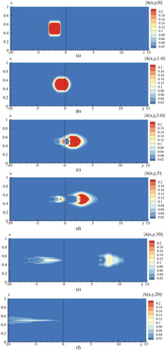
Figure 6. Square root from beam profile $|A{|}^2$ along y-coordinate at the beam axis on x-coordinate (x = 0.5) at time moment t = 0 (a), 1.4 (b), 3.6(c), 5(d), 10(e), 20(f).

Figure 7. Distribution of free-electron concentration n at time moment t = 3.2 (a), 3.4 (b), 3.6 (c), 4 (d), 5 (e), 10 (f).

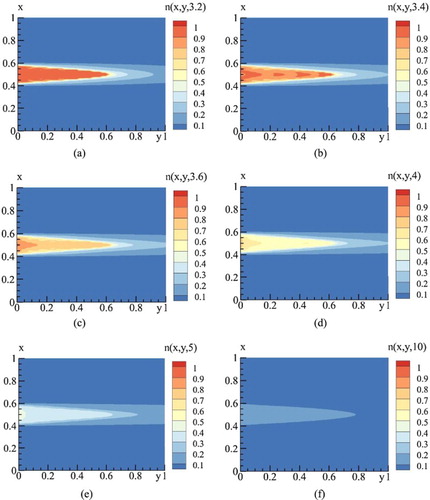
Figure 8. Square root from beam profile $|A{|}^2$ along y-coordinate at the beam axis on x-coordinate (x = 0.5) at time moment t = 1.4 (a), 3 (b), 3.6(c), 5(d), 10(e), 20(f).

We see in Figure 5 that a part of laser beam reflects from a semiconductor face in time moment $t=3.6$. The laser beam transmitted through a boundary of a semiconductor with air acquires very complicated profile. The travelling part of the beam penetrated in a semiconductor becomes with intensity minimum at the x-axis near the face of a semiconductor (Figure 5(b,c)). With time increasing, the beam profile becomes much more disturbed one in comparison with the incident Gaussian profile. The reflected beam possesses also complicated profile in the x-direction as well as in y-direction. (Figure 5(d)). A part of the reflected beam moves faster than other ones (Figure 6). For the beam propagating in a semiconductor, the pulse front moves faster than a basic part of the beam. For illustration of the complicated spatial–temporal intensity distribution, in Figure 6 the beam profile along y-coordinate at beam axis on x-coordinate is depicted at various time moments. We see a formation of the laser sub-pulses propagating in both directions along y-coordinate.

Analysis of the free-electron spatial–temporal distribution (Figure 7) shows that the laser beam diffraction action results in multi-domains formation for high absorption (Figure 7(b,c)). We see an appearance of the free-electron high concentration domains on both coordinates (Figure 7(b)). For example, such domains form in the section y = 0.12 which cannot appear without taking into account the beam diffraction.

Figure 8 illustrates the influence of the reflected optical pulse from the high concentration domain. As a result of this, we see that the pulse intensity increases near the face of the semiconductor with increasing time.

In Table 1 the values of invariant (79) and the difference analogue of integral equality (29) (184) $\overline{\overline{Q}}\left(t_m\right)=\sum _{j=-P_y+1}^{P_y-1}\sum _{k=1}^{P_x-1}{h}_y{h}_x\left(\frac{{|{\hat{A}}_{kj}^m|}^2-{|A_{kj}^m|}^2}{\tau }+{\beta }_A{\delta }_{0_h}\stackrel{0.5}{\delta }\stackrel{0.5}{{|A_{kj}^m|}^2}\right)$(184) are shown. It should be noticed, that invariant (29) approximated by formula (184) with the second order on spatial and time coordinates. As we can see, both characteristics $Q\left(t_m\right)$ and $\overline{\overline{Q}}\left(t_m\right)$ preserve their values with high accuracy. Thus, a conservatism property which was proved analytically in Theorem 3.1 is confirmed also by computer simulation. It means, that our numerical method allows providing computations on long time interval without accumulating the rounding errors and this method possesses the asymptotic stability property.

Table 1. Invariants $Q\left(t_m\right)$ and $\overline{\overline{Q}}\left(t_m\right)$ values computed using formulas (79) and (184), correspondingly.

$t_m$	Invariant $Q\left(t_m\right)$	Invariant $\overline{\overline{Q}}\left(t_m\right)$
1.4	2.81732e−06	1.11856e−07
3.6	1.56882e−05	1.5281e−06
4	1.95336e−05	1.09616e−06
5	1.54824e−05	6.44219e−07
10	8.78868e−06	9.8865e−08

6. Conclusions

A new mathematical model for the resonatorless OB scheme based on a semiconductor is proposed. The main feature of this model consists in taking into account the longitudinal diffraction of the optical beam. Its action results in a laser beam reflection from the boundaries of high absorption domains. The transverse diffraction induces the laser beam reshaping.

To solve the 2D nonlinear Schrödinger equation together with the set of the equations describing an electron–hole plasma evolution in a semiconductor, the conservative FDS on the base of Crank–Nicolson scheme is proposed and its conservatism is proved. For its realization, the two-stage iteration process is used. Such iteration method allows to achieve the conservatism property on each of the iterations.

We showed the uniform boundedness of the mesh functions at the iterations, the convergence of the iteration process. We showed also positiveness and boundedness of the mesh function corresponding to free-charged particle concentrations. We discuss some properties of the differential problem including the problem invariants, positiveness of the free-charge concentrations.

Disclosure statement

No potential conflict of interest was reported by the authors.

Additional information

Funding

This paper was made using the support of the Russian Science Foundation [grant number 14-21-00081].

References

- G. Bachman and L. Narici, Functional Analysis, Dover Publications, Inc., Mineola, NY, 1998.
- L. Barletti, L. Brugnano, G. Frasca Caccia, and F. Iavernaro, Energy-conserving methods for the nonlinear Schrödinger equation, Appl. Math. Comput. 318 (2018), pp. 3–18.
- O.S. Bondarenko, Mathematical modeling of some problems of optical bistability on the basis of semiconductors, PhD thesis (1997) (in Russian).
- M. Dehghan and A. Taleei, A compact split-step finite difference method for solving the nonlinear Schrödinger equations with constant and variable coefficients, Comput. Phys. Commun. 181 (2010), pp. 43–51. doi: 10.1016/j.cpc.2009.08.015
- J.I. Dıaz and G. Galiano, Existence and uniqueness of solutions of the Boussinesq system with nonlinear thermal diffusion, topological methods in nonlinear analysis, J. Juliusz Schauder Center 11 (1998), pp. 59–82.
- D. Dockery and J.R. Kuttler, An improved impedance-boundary algorithm for Fourier split-step solutions of the parabolic wave equation, IEEE Trans. Antennas Propag. 44 (1996), pp. 1592–1599. doi: 10.1109/8.546245
- A. Friedman, Partial Differential Equations of Parabolic Type, Dover Publications, Inc., Mineola, NY, 2008.
- A. Ghadi and S. Mirzanejhad, Two-photon absorption effect on semiconductor microring resonators, Optik (Stuttg) 126 (2015), pp. 1645–1649. doi: 10.1016/j.ijleo.2015.05.058
- H.M. Gibbs, Optical Bistability: Controlling Light with Light, Academic Press, New York, 1985.
- H.M. Gibbs, S.L. McCall, and T.N.C. Venkatesan, Optical bistable devices – the basic components of all-optical systems, Opt. Eng. 19(4) (1980), pp. 463–468. doi: 10.1117/12.7972544
- H.M. Gibbs, S.L. McCall, T.N.C. Venkatesan, A.C. Gossard, A. Passner, and W. Wiegmann, Optical bistability in semiconductors, Appl. Phys. Lett. 35(6) (1979), pp. 451–453. doi: 10.1063/1.91157
- W. Huang, M. Ji, Z. Liu, and Y. Yi, Steady states of Fokker–Planck equations: I. Existence, J. Dynam. Differential Equations 27 (3–4) (2015), pp. 721–742.doi: 10.1007/s10884-015-9454-x
- A. Hurtado, M. Nami, I. D. Henning, M.G. Adams, and L.F. Lester, Bistability patterns and nonlinear switching with very high contrast ratio in a 1550 nm quantum dash semiconductor laser, Appl. Phys. Lett. 101 (2012), pp. 161117. doi: 10.1063/1.4761473
- Yu N. Karamzin, A.P. Sukhorukov, and V.A. Trofimov, Mathematical Modeling in Nonlinear Optics, Moscow University Publishing, Moscow, 1989, p. 156 (in Russian).
- P.K. Kwan and Y.Y. Lu, Computing optical bistability in one-dimensional nonlinear structures, Optics Commun. 238 (2004), pp. 169–175. doi: 10.1016/j.optcom.2004.04.025
- O. Ladyzhenskaya and N.N. Uraltseva, Linear and Quasilinear Elliptic Equations, Nauka, Moscow, 1973 (in Russian).
- T.I. Lakoba, Instability of the finite-difference split-step method applied to the generalized nonlinear Schrödinger equation. III. External potential and oscillating pulse solutions, Numer. Methods Partial Differential Equations, 33 (2017) pp. 633–650. doi: 10.1002/num.22071
- A.W. Leung, Nonlinear Systems of Partial Differential Equations: Applications to Life and Physical Sciences, Word Scientific Publishing Co. Pvt. Ltd, Hackensack, NJ, 2009.
- L. Li, Optical bistability in semiconductor lasers under intermodal light injection, J.f Quantum Electronics 32 (1996), pp. 248–256. doi: 10.1109/3.481872
- J. Loustau, Numerical Differential Equations: Theory and Technique,ode Methods, Finite Differences, Finite Elements and Collocation, WordScientific Publishing Co. Pte. Ltd., New Jersey, 2016.
- G.I. Marchuk, Methods of Numerical Mathematics, New York, NY, Springer, 1975.
- J.D. Murray, Mathematical Biology II: Spatial Models and Biomedical Application, Springer-Verlag, New York, 2003.
- R. Nasehi, Ultra-low threshold optical bistability and multi-stability in dielectric slab doped with semiconductor quantum well, Commun. Theor. Phys. 66 (2016), pp. 129–132. doi: 10.1088/0253-6102/66/1/129
- A.A. Samarskii, Difference Schemes Theory, Nauka, Moscow, 1977 (in Russian).
- A.A. Samarskii, V.A. Galaktionov, S.P. Kurdumov, and A.P. Mikhailov, The Modes with Aggravation in Problems for the Quasilinear and Parabolic Equations, Nauka, Moscow, 1987 (in Russian).
- R.A. Smith, Semiconductors, Cambridge Univ. Press, Cambridge, 1978.
- G. Strang, On the construction and comparison of difference schemes, SIAM J. Numer. Anal. 5 (3) (1968), pp. 506–517. doi: 10.1137/0705041
- A. Suryanto, E. van Groesen, and M. Hammer, Finite element analysis of optical bistability in one-dimensional nonlinear photonic band gap structures with a defect, J. Nonlinear Optic. Phys. Mater. 12 (2003), pp. 187. doi: 10.1142/S0218863503001328
- A. Taleei and M. Dehghan, Time-splitting pseudo-spectral domain decomposition method for the soliton solutions of the one- and multi-dimensional nonlinear Schrödinger equations, Comput. Phys. Commun. 185 (2014), pp. 1515–1528. doi: 10.1016/j.cpc.2014.01.013
- Z. Toroker and M. Horowit, Optimized split-step method for modeling nonlinear pulse propagation in fiber Bragg gratings, JOSA B 25 (2008), pp. 448–457. doi: 10.1364/JOSAB.25.000448
- S. K. Tripathy and S. Swain, Optical bistable switching in semiconductor heterostructure containing a quantum dot layer: The effect of phonons, Optik (Stuttg) 124 (2013), pp. 2723–2726. doi: 10.1016/j.ijleo.2012.08.088
- V.A. Trofimov, M.M. Loginova, and V.A. Egorenkov, 2D wave structure induced by femtosecond laser pulse in semiconductor, Adv. Optoelectronics Lasers, Kharkov (2013), pp. 296–298.
- V.A. Trofimov, M.M. Loginova, and V.A. Egorenkov, Developing of 2D helical waves in semiconductor under the action of femtosecond laser pulse and external electric field, Proc. SPIE, 9586 (2015), 95860 K. doi: 10.1117/12.2189308
- V.A. Trofimov, M.M. Loginova, and V.A. Egorenkov, New two-step iteration process for solution of semiconductor plasma generation problem with arbitrary boundary conditions in 2D case, WIT trans. Model. Simul. 59 (2015), pp. 85–96.
- V.A. Trofimov, M.M. Loginova, and V.A. Egorenkov, Conservative finite-difference scheme for computer simulation of field optical bistability, Lecture Notes Comput. Sci. 10187 (2017), pp. 682–689. doi: 10.1007/978-3-319-57099-0_78
- H. Wang, Numerical studies on the split-step finite difference method for nonlinear Schrödinger equations, Appl. Math. Comput. 170 (2005), pp. 17–35.
- H. Wang, X. Ma, J. Lu, and W. Gao, An efficient time-splitting compact finite difference method for gross–Pitaevskii equation, Appl. Math. Comput. 297 (2017), pp. 131–144.
- H. Wang, H.-T. Zhang, and Z.-P. Wang, Optical bistability via incoherent pumping fields in semiconductor quantum wells, Mod Phys Lett B 25 (2011), pp. 97.
- D. Weaire and J. P. Kermode, Dispersive optical bistability – numerical methods and definitive results, JOSA B 3 (1986), pp. 1706–1711. doi: 10.1364/JOSAB.3.001706
- J.A.C. Weideman and B.M. Herbst, Split-step methods for the solution of the nonlinear Schrödinger equation, SIAM J. Numer. Anal. 23 (1986), pp. 485–507. doi: 10.1137/0723033