Drift-preserving numerical integrators for stochastic Poisson systems

Abstract

We perform a numerical analysis of a class of randomly perturbed Hamiltonian systems and Poisson systems. For the considered additive noise perturbation of such systems, we show the long-time behaviour of the energy and quadratic Casimirs for the exact solution. We then propose and analyse a drift-preserving splitting scheme for such problems with the following properties: exact drift preservation of energy and quadratic Casimirs, mean-square order of convergence 1, weak order of convergence 2. These properties are illustrated with numerical experiments.

Keywords:

• Stochastic differential equations
• stochastic Hamiltonian systems
• stochastic Poisson systems
• energy
• Casimir
• trace formula
• numerical schemes
• strong convergence
• weak convergence

2020 Mathematics Subject Classifications:

• 65C30
• 65P10
• 60H10
• 60H35

1. Introduction

Hamiltonian systems are widely used models in science and engineering. In the deterministic case, one main feature of such models is that the solution conserves exactly the Hamiltonian energy for all times. The design and study of energy-preserving numerical methods for such problems has attracted much attention in the recent years, see for instance [7,8,12,17,22,23,29,30,34,37–39,49] and references therein.

For an additive white noise perturbation of such Hamiltonian systems, the energy is no longer constant along time, but grows in average linearly for the exact solution, which reveals non trivial to reproduce by numerical methods, see [9,13,14,19,21,28,43,44], and extensions to the case of stochastic partial differential equations in [3,4,15,18,41].

In this paper, we propose and analyse a drift-preserving scheme for stochastic Poisson systems subject to an additive noise perturbation. Such problems are a direct generalization of the stochastic differential equations (SDEs) studied recently in [13], as well as in all the above references, but the proposed numerical integrator is not a trivial generalization of the one given in [13].

In Section 2, we propose a new numerical method that exactly satisfies a trace formula for the linear growth for all times of the expected value of the Hamiltonian energy and of the Casimir of the solution. Such long-time behaviour corresponds to the one of the exact solution of stochastic Poisson systems and can also be seen as a long-time weak convergence estimate. For the sake of completeness, in Section 3, we prove mean-square and weak orders of convergence of the proposed numerical method under classical assumptions on the coefficients of the problem. Finally, Section 4 is devoted to numerical experiments illustrating the main properties of the new numerical method for stochastic Hamiltonian systems and Poisson systems.

2. Drift-preserving scheme for stochastic Poisson problem

This section presents the problem, introduces the drift-preserving integrator and shows some of its main geometric properties.

2.1. Setting

For a fixed dimension d, let $W(t)\in {\mathbb{R}}^d$ denote a standard d-dimensional Wiener process defined for t>0 on a probability space equipped with a filtration and fulfilling the usual assumptions. For a fixed dimension m and a smooth potential $V:{\mathbb{R}}^m\to \mathbb{R}$, we consider the separable Hamiltonian function of the form (1) $H(p,q)=\frac{1}{2}\sum _{j=1}^m{p}_j^2+V(q).$(1) We next set $X(t)=(p(t),q(t))\in {\mathbb{R}}^m\times {\mathbb{R}}^m$ and consider the following stochastic Poisson system with additive noise (2) $\mathrm{d}X(t)=B(X(t))\mathrm{\nabla }H(X(t))\mathrm{d}t+\left(\begin{array}{c}\mathrm{\Sigma }\\ 0\end{array}\right)\mathrm{d}W(t).$(2) Here, $B(X)\in {\mathbb{R}}^{2m\times 2m}$ is a smooth skew-symmetric matrix and $\mathrm{\Sigma }\in {\mathbb{R}}^{m\times d}$ is a constant matrix. The initial value $X_0=(p_0,q_0)$ of the problem (2(2) $\mathrm{d}X(t)=B(X(t))\mathrm{\nabla }H(X(t))\mathrm{d}t+\left(\begin{array}{c}\mathrm{\Sigma }\\ 0\end{array}\right)\mathrm{d}W(t).$(2) ) is assumed to be either non-random or a random variable with bounded moments up to any order (and adapted to the filtration). For simplicity, we assume in the analysis of this paper that $(x,y)\mapsto B(x)\mathrm{\nabla }H(y)$ is globally Lipschitz continuous on ${\mathbb{R}}^{2m}\times {\mathbb{R}}^{2m}$ and that H and B are $C^7$, resp. $C^6$-functions with all partial derivatives with at most polynomial growth. This is to ensure existence and uniqueness of solutions to (2(2) $\mathrm{d}X(t)=B(X(t))\mathrm{\nabla }H(X(t))\mathrm{d}t+\left(\begin{array}{c}\mathrm{\Sigma }\\ 0\end{array}\right)\mathrm{d}W(t).$(2) ) for all times t>0 as well as bounded moments at any orders of such solutions. These regularity assumptions on the coefficients B and H will also be used to show strong and weak convergence of the proposed numerical scheme for (2(2) $\mathrm{d}X(t)=B(X(t))\mathrm{\nabla }H(X(t))\mathrm{d}t+\left(\begin{array}{c}\mathrm{\Sigma }\\ 0\end{array}\right)\mathrm{d}W(t).$(2) ). We observe that one could weaken these assumptions, but this is not the aim of the present work. The present setting covers, for instance, the following examples: simplified versions of the stochastic rigid bodies studied in [45,47], the stochastic Hamiltonian systems considered in [13] by taking $B(X)=J=\left(\begin{array}{cc}0& -I{d}_m\\ I{d}_m& 0\end{array}\right)$the constant canonical symplectic matrix, for which the SDE (2(2) $\mathrm{d}X(t)=B(X(t))\mathrm{\nabla }H(X(t))\mathrm{d}t+\left(\begin{array}{c}\mathrm{\Sigma }\\ 0\end{array}\right)\mathrm{d}W(t).$(2) ) yields $\mathrm{d}p(t)=-\mathrm{\nabla }V(q(t))\mathrm{d}t+\mathrm{\Sigma }\mathrm{d}W(t),\mathrm{d}q(t)=p(t)\mathrm{d}t,$the Hamiltonian considered in [9] (where the matrix Σ is diagonal), the linear stochastic oscillator from [44], and various stochastic Hamiltonian systems studied in [36, Chap. 4], see also [35], or [26,27,42,50].

Remark 2.1

We emphasize that our analysis is not restricted to the above form of the Hamiltonian. Indeed, the results below as well as the proposed numerical scheme can be applied to the more general problem (no needed of partitioning the vector X neither to have the separable Hamiltonian (1(1) $H(p,q)=\frac{1}{2}\sum _{j=1}^m{p}_j^2+V(q).$(1) )) $\mathrm{d}X(t)=B(X(t))\mathrm{\nabla }H(X(t))\mathrm{d}t+\left(\begin{array}{c}\mathrm{\Sigma }\\ 0\end{array}\right)\mathrm{d}W(t),$as long as the Hessian of the Hamiltonian has a nice structure. One could for instance consider a (linear in p) term of the form $\tilde{V}(q)p$ or most importantly the case when the Hamiltonian is quadratic as in the example of a stochastic rigid body problem. See below for further details.

Applying Itô's lemma to the function $H(X)$ on the solution process $X(t)$ of (2(2) $\mathrm{d}X(t)=B(X(t))\mathrm{\nabla }H(X(t))\mathrm{d}t+\left(\begin{array}{c}\mathrm{\Sigma }\\ 0\end{array}\right)\mathrm{d}W(t).$(2) ), one obtains (3) $\begin{array}{rl}\mathrm{d}H(X(t))& =(\mathrm{\nabla }H(X(t){)}^{\mathrm{\top }}B(X(t))\mathrm{\nabla }H(X(t))+\frac{1}{2}\mathrm{Tr}\left({\left(\begin{array}{c}\mathrm{\Sigma }\\ 0\end{array}\right)}^{\mathrm{\top }}{\mathrm{\nabla }}^{2}H\left(\begin{array}{c}\mathrm{\Sigma }\\ 0\end{array}\right)\right))\mathrm{d}t\\ & +\mathrm{\nabla }H(X(t){)}^{\mathrm{\top }}\left(\begin{array}{c}\mathrm{\Sigma }\\ 0\end{array}\right)\mathrm{d}W(t).\end{array}$(3) Using the skew-symmetry of the matrix $B(X)$, we have $\mathrm{\nabla }H(X{)}^{T}B(X)\mathrm{\nabla }H(X)=0$. Furthermore, using that the partial Hessian ${\mathrm{\nabla }}_{pp}^{2}H(X)=I{d}_m$ is a constant matrix, thanks to the separable form of the Hamiltonian (1(1) $H(p,q)=\frac{1}{2}\sum _{j=1}^m{p}_j^2+V(q).$(1) ), and rewriting the above equation in integral form and taking the expectation, one finally obtains the so-called trace formula for the energy of the stochastic Poisson SDE (2(2) $\mathrm{d}X(t)=B(X(t))\mathrm{\nabla }H(X(t))\mathrm{d}t+\left(\begin{array}{c}\mathrm{\Sigma }\\ 0\end{array}\right)\mathrm{d}W(t).$(2) ): (4) $\mathbb{E}[H(X(t))]=\mathbb{E}[H(X_0)]+\frac{1}{2}\mathrm{Tr}\left({\mathrm{\Sigma }}^{\mathrm{\top }}\mathrm{\Sigma }\right)t.$(4) This shows that the expected energy of the exact solution of (2(2) $\mathrm{d}X(t)=B(X(t))\mathrm{\nabla }H(X(t))\mathrm{d}t+\left(\begin{array}{c}\mathrm{\Sigma }\\ 0\end{array}\right)\mathrm{d}W(t).$(2) ) grows linearly with time for all t>0.

Remark 2.2

Observe that the form of the noise term in equation (2(2) $\mathrm{d}X(t)=B(X(t))\mathrm{\nabla }H(X(t))\mathrm{d}t+\left(\begin{array}{c}\mathrm{\Sigma }\\ 0\end{array}\right)\mathrm{d}W(t).$(2) ) makes the term $\mathrm{Tr}\left({\left(\begin{array}{c}\mathrm{\Sigma }\\ 0\end{array}\right)}^{\mathrm{\top }}{\mathrm{\nabla }}^{2}H\left(\begin{array}{c}\mathrm{\Sigma }\\ 0\end{array}\right)\right)=\mathrm{Tr}\left({\mathrm{\Sigma }}^{\mathrm{\top }}\mathrm{\Sigma }\right)$in (3(3) $\begin{array}{rl}\mathrm{d}H(X(t))& =(\mathrm{\nabla }H(X(t){)}^{\mathrm{\top }}B(X(t))\mathrm{\nabla }H(X(t))+\frac{1}{2}\mathrm{Tr}\left({\left(\begin{array}{c}\mathrm{\Sigma }\\ 0\end{array}\right)}^{\mathrm{\top }}{\mathrm{\nabla }}^{2}H\left(\begin{array}{c}\mathrm{\Sigma }\\ 0\end{array}\right)\right))\mathrm{d}t\\ & +\mathrm{\nabla }H(X(t){)}^{\mathrm{\top }}\left(\begin{array}{c}\mathrm{\Sigma }\\ 0\end{array}\right)\mathrm{d}W(t).\end{array}$(3) ) independent of the stochastic process $X(t)$. Hence one obtains the linear growth along time of the expected energy in (4(4) $\mathbb{E}[H(X(t))]=\mathbb{E}[H(X_0)]+\frac{1}{2}\mathrm{Tr}\left({\mathrm{\Sigma }}^{\mathrm{\top }}\mathrm{\Sigma }\right)t.$(4) ). In general, this is not the case if one would consider a non-zero additive noise in all the component or a multiplicative noise in (2(2) $\mathrm{d}X(t)=B(X(t))\mathrm{\nabla }H(X(t))\mathrm{d}t+\left(\begin{array}{c}\mathrm{\Sigma }\\ 0\end{array}\right)\mathrm{d}W(t).$(2) ). Note however that the linear growth property of the expected energy is still valid if one considers a more general Hamiltonian function (1(1) $H(p,q)=\frac{1}{2}\sum _{j=1}^m{p}_j^2+V(q).$(1) ) with kinetic energy given by $\frac{1}{2}{p}^{\mathrm{\top }}{M}^{-1}p$, with a given invertible mass matrix M.

Our objective is to derive and analyse a new numerical scheme for (2(2) $\mathrm{d}X(t)=B(X(t))\mathrm{\nabla }H(X(t))\mathrm{d}t+\left(\begin{array}{c}\mathrm{\Sigma }\\ 0\end{array}\right)\mathrm{d}W(t).$(2) ) that possesses the same trace formula for the energy for all times.

2.2. Definition of the numerical scheme

The numerical integrator studied in [13] cannot directly be applied to the stochastic Poisson system (2(2) $\mathrm{d}X(t)=B(X(t))\mathrm{\nabla }H(X(t))\mathrm{d}t+\left(\begin{array}{c}\mathrm{\Sigma }\\ 0\end{array}\right)\mathrm{d}W(t).$(2) ). Our idea is to combine a splitting scheme with one of the (deterministic) energy-preserving schemes from [17]. Observe that a similar strategy was independently presented in [20] in the particular context of the Langevin equation with other aims than here. We thus propose the following time integrator for problem (2(2) $\mathrm{d}X(t)=B(X(t))\mathrm{\nabla }H(X(t))\mathrm{d}t+\left(\begin{array}{c}\mathrm{\Sigma }\\ 0\end{array}\right)\mathrm{d}W(t).$(2) ), which is shown in Theorem 2.2 to be a drift-preserving integrator for all times: (5) $\begin{array}{rl}{Y}_1& :=X_n+\left(\begin{array}{c}\mathrm{\Sigma }\\ 0\end{array}\right)(W(t_n+\frac{h}{2})-W(t_n)),\\ Y_2& :=Y_1+hB\left(\frac{Y_1+Y_2}{2}\right){\int }_0^1\mathrm{\nabla }H(Y_1+\theta (Y_2-Y_1))\mathrm{d}\theta ,\\ X_{n+1}& =Y_2+\left(\begin{array}{c}\mathrm{\Sigma }\\ 0\end{array}\right)(W(t_{n+1})-W(t_n+\frac{h}{2})).\end{array}$(5) In the above formulas, we denote the step size of the drift-preserving scheme with h>0 and discrete times with $t_n=nh$.

Remark 2.3

(Numerical implementation) The middle step in Equation (5(5) $\begin{array}{rl}{Y}_1& :=X_n+\left(\begin{array}{c}\mathrm{\Sigma }\\ 0\end{array}\right)(W(t_n+\frac{h}{2})-W(t_n)),\\ Y_2& :=Y_1+hB\left(\frac{Y_1+Y_2}{2}\right){\int }_0^1\mathrm{\nabla }H(Y_1+\theta (Y_2-Y_1))\mathrm{d}\theta ,\\ X_{n+1}& =Y_2+\left(\begin{array}{c}\mathrm{\Sigma }\\ 0\end{array}\right)(W(t_{n+1})-W(t_n+\frac{h}{2})).\end{array}$(5) ) requires, in general, the solution to a nonlinear system of equations. Even in higher dimension, if the problem is not stiff, this can be solved by fixed point iterations rather than Newton iterations, which makes the computational complexity similar to that of an implicit Runge–Kutta scheme with two stages, see [17, Section 2.2] or [24, Chapter VIII.6] for instance.

Remark 2.4

(Further extensions) Let us observe that the (deterministic) energy-preserving scheme from [17] present in the term in the middle of (5(5) $\begin{array}{rl}{Y}_1& :=X_n+\left(\begin{array}{c}\mathrm{\Sigma }\\ 0\end{array}\right)(W(t_n+\frac{h}{2})-W(t_n)),\\ Y_2& :=Y_1+hB\left(\frac{Y_1+Y_2}{2}\right){\int }_0^1\mathrm{\nabla }H(Y_1+\theta (Y_2-Y_1))\mathrm{d}\theta ,\\ X_{n+1}& =Y_2+\left(\begin{array}{c}\mathrm{\Sigma }\\ 0\end{array}\right)(W(t_{n+1})-W(t_n+\frac{h}{2})).\end{array}$(5) ) could be replaced by another (deterministic) energy-preserving scheme for (deterministic) Poisson systems, see for example: [6,8,10,48] or a straightforward adaptation of the energy-preserving Runge–Kutta schemes for polynomial Hamiltonians in [11]. Let us further remark that it is also possible to interchange the ordering in the splitting scheme by considering first half a step of the (deterministic) energy-preserving scheme, then a full step of the stochastic part, and finally again half a step of the (deterministic) energy-preserving scheme. Finally, let us add that one could add a damping term in the SDE (2(2) $\mathrm{d}X(t)=B(X(t))\mathrm{\nabla }H(X(t))\mathrm{d}t+\left(\begin{array}{c}\mathrm{\Sigma }\\ 0\end{array}\right)\mathrm{d}W(t).$(2) ) to compensate for the drift in the energy thus getting conservation of energy for such problems (either in average or a.s.). In this case, one would add the damping term in the first and last equations of the numerical scheme (5(5) $\begin{array}{rl}{Y}_1& :=X_n+\left(\begin{array}{c}\mathrm{\Sigma }\\ 0\end{array}\right)(W(t_n+\frac{h}{2})-W(t_n)),\\ Y_2& :=Y_1+hB\left(\frac{Y_1+Y_2}{2}\right){\int }_0^1\mathrm{\nabla }H(Y_1+\theta (Y_2-Y_1))\mathrm{d}\theta ,\\ X_{n+1}& =Y_2+\left(\begin{array}{c}\mathrm{\Sigma }\\ 0\end{array}\right)(W(t_{n+1})-W(t_n+\frac{h}{2})).\end{array}$(5) ) in order to get a (stochastic) energy-preserving splitting scheme. An example of application is Langevin's equation, a widely studied model in the context of molecular dynamics. We do not pursue further this question.

We now show the boundedness along time of all moments of the numerical solution given by (5(5) $\begin{array}{rl}{Y}_1& :=X_n+\left(\begin{array}{c}\mathrm{\Sigma }\\ 0\end{array}\right)(W(t_n+\frac{h}{2})-W(t_n)),\\ Y_2& :=Y_1+hB\left(\frac{Y_1+Y_2}{2}\right){\int }_0^1\mathrm{\nabla }H(Y_1+\theta (Y_2-Y_1))\mathrm{d}\theta ,\\ X_{n+1}& =Y_2+\left(\begin{array}{c}\mathrm{\Sigma }\\ 0\end{array}\right)(W(t_{n+1})-W(t_n+\frac{h}{2})).\end{array}$(5) ).

Lemma 2.1

Let T>0. Apply the drift-preserving numerical scheme (5(5) $\begin{array}{rl}{Y}_1& :=X_n+\left(\begin{array}{c}\mathrm{\Sigma }\\ 0\end{array}\right)(W(t_n+\frac{h}{2})-W(t_n)),\\ Y_2& :=Y_1+hB\left(\frac{Y_1+Y_2}{2}\right){\int }_0^1\mathrm{\nabla }H(Y_1+\theta (Y_2-Y_1))\mathrm{d}\theta ,\\ X_{n+1}& =Y_2+\left(\begin{array}{c}\mathrm{\Sigma }\\ 0\end{array}\right)(W(t_{n+1})-W(t_n+\frac{h}{2})).\end{array}$(5) ) to the Poisson system with additive noise (2(2) $\mathrm{d}X(t)=B(X(t))\mathrm{\nabla }H(X(t))\mathrm{d}t+\left(\begin{array}{c}\mathrm{\Sigma }\\ 0\end{array}\right)\mathrm{d}W(t).$(2) ) on the compact time interval $[0,T]$. One then has the following bounds for the numerical moments: for all step sizes h assumed small enough and all $m\in \mathbb{N}$, $\mathbb{E}[|X_n{|}^{2m}]\le C_m,$for all $t_n=nh\le T$, where $C_m$ is independent of n and h.

Proof.

To show boundedness of the moments of the numerical solution given by (5(5) $\begin{array}{rl}{Y}_1& :=X_n+\left(\begin{array}{c}\mathrm{\Sigma }\\ 0\end{array}\right)(W(t_n+\frac{h}{2})-W(t_n)),\\ Y_2& :=Y_1+hB\left(\frac{Y_1+Y_2}{2}\right){\int }_0^1\mathrm{\nabla }H(Y_1+\theta (Y_2-Y_1))\mathrm{d}\theta ,\\ X_{n+1}& =Y_2+\left(\begin{array}{c}\mathrm{\Sigma }\\ 0\end{array}\right)(W(t_{n+1})-W(t_n+\frac{h}{2})).\end{array}$(5) ), we use [36, Lemma 2.2, p. 102], which states that it is sufficient to show the following estimates: $\left|\mathbb{E}[X_{n+1}-X_n|X_n]\right|\le C(1+|X_n|)h\mathrm{and}|X_{n+1}-X_n|\le M_n(1+|X_n|)\sqrt{h},$where C is independent of h and $M_n$ is a random variable with moments of all orders bounded uniformly with respect to all h small enough. Since the numerical scheme (5(5) $\begin{array}{rl}{Y}_1& :=X_n+\left(\begin{array}{c}\mathrm{\Sigma }\\ 0\end{array}\right)(W(t_n+\frac{h}{2})-W(t_n)),\\ Y_2& :=Y_1+hB\left(\frac{Y_1+Y_2}{2}\right){\int }_0^1\mathrm{\nabla }H(Y_1+\theta (Y_2-Y_1))\mathrm{d}\theta ,\\ X_{n+1}& =Y_2+\left(\begin{array}{c}\mathrm{\Sigma }\\ 0\end{array}\right)(W(t_{n+1})-W(t_n+\frac{h}{2})).\end{array}$(5) ) is a splitting method, it is more convenient to apply [36, Lemma 2.2, p. 102] to the Markov chain $\{X_0,Y_1,Y_2,X_1,\dots \}$ instead of the Markov chain $\{X_0,X_1,\dots \}$. This makes the verification of the above estimates immediate using the linear growth property of the coefficients of the SDE (2(2) $\mathrm{d}X(t)=B(X(t))\mathrm{\nabla }H(X(t))\mathrm{d}t+\left(\begin{array}{c}\mathrm{\Sigma }\\ 0\end{array}\right)\mathrm{d}W(t).$(2) ), a consequence of their Lipschitzness.

2.3. Exact drift preservation of energy

We are now in position to prove the main feature of the proposed numerical method (5(5) $\begin{array}{rl}{Y}_1& :=X_n+\left(\begin{array}{c}\mathrm{\Sigma }\\ 0\end{array}\right)(W(t_n+\frac{h}{2})-W(t_n)),\\ Y_2& :=Y_1+hB\left(\frac{Y_1+Y_2}{2}\right){\int }_0^1\mathrm{\nabla }H(Y_1+\theta (Y_2-Y_1))\mathrm{d}\theta ,\\ X_{n+1}& =Y_2+\left(\begin{array}{c}\mathrm{\Sigma }\\ 0\end{array}\right)(W(t_{n+1})-W(t_n+\frac{h}{2})).\end{array}$(5) ) which benefits from the very same trace formula for the energy as the one for the exact solution to the stochastic Poisson problem (2(2) $\mathrm{d}X(t)=B(X(t))\mathrm{\nabla }H(X(t))\mathrm{d}t+\left(\begin{array}{c}\mathrm{\Sigma }\\ 0\end{array}\right)\mathrm{d}W(t).$(2) ), hence the name drift-preserving integrator for this numerical scheme.

Theorem 2.2

Consider the numerical scheme (5(5) $\begin{array}{rl}{Y}_1& :=X_n+\left(\begin{array}{c}\mathrm{\Sigma }\\ 0\end{array}\right)(W(t_n+\frac{h}{2})-W(t_n)),\\ Y_2& :=Y_1+hB\left(\frac{Y_1+Y_2}{2}\right){\int }_0^1\mathrm{\nabla }H(Y_1+\theta (Y_2-Y_1))\mathrm{d}\theta ,\\ X_{n+1}& =Y_2+\left(\begin{array}{c}\mathrm{\Sigma }\\ 0\end{array}\right)(W(t_{n+1})-W(t_n+\frac{h}{2})).\end{array}$(5) ) applied to the Poisson system with additive noise (2(2) $\mathrm{d}X(t)=B(X(t))\mathrm{\nabla }H(X(t))\mathrm{d}t+\left(\begin{array}{c}\mathrm{\Sigma }\\ 0\end{array}\right)\mathrm{d}W(t).$(2) ). Then, for all time steps h assumed small enough, the expected energy of the numerical solution satisfies the following trace formula: (6) $\mathbb{E}[H(X_n)]=\mathbb{E}[H(X_0)]+\frac{1}{2}\mathrm{Tr}\left({\mathrm{\Sigma }}^{\mathrm{\top }}\mathrm{\Sigma }\right)t_n$(6) for all discrete times $t_n=nh$, where $n\in \mathbb{N}$.

Proof.

The first step of the drift-preserving scheme can be rewritten as $Y_1=X_n+{\int }_{t_n}^{t_n+\frac{h}{2}}\left(\begin{array}{c}\mathrm{\Sigma }\\ 0\end{array}\right)\mathrm{d}W(s)$and an application of Itô's formula gives $\mathbb{E}[H(Y_1)]=\mathbb{E}[H(X_n)]+\frac{h}{4}\mathrm{Tr}\left({\mathrm{\Sigma }}^{\mathrm{\top }}\mathrm{\Sigma }\right).$Since the second step of the drift-preserving scheme (5(5) $\begin{array}{rl}{Y}_1& :=X_n+\left(\begin{array}{c}\mathrm{\Sigma }\\ 0\end{array}\right)(W(t_n+\frac{h}{2})-W(t_n)),\\ Y_2& :=Y_1+hB\left(\frac{Y_1+Y_2}{2}\right){\int }_0^1\mathrm{\nabla }H(Y_1+\theta (Y_2-Y_1))\mathrm{d}\theta ,\\ X_{n+1}& =Y_2+\left(\begin{array}{c}\mathrm{\Sigma }\\ 0\end{array}\right)(W(t_{n+1})-W(t_n+\frac{h}{2})).\end{array}$(5) ) is the deterministic energy-preserving scheme from [17], one then obtains $\mathbb{E}[H(Y_2)]=\mathbb{E}[H(Y_1)].$Finally, as in the beginning of the proof, the last step of the numerical integrator provides $\begin{array}{rl}\mathbb{E}[H(X_{n+1})]& =\mathbb{E}[H(Y_2)]+\frac{h}{4}\mathrm{Tr}\left({\mathrm{\Sigma }}^{\mathrm{\top }}\mathrm{\Sigma }\right)=\mathbb{E}[H(Y_1)]+\frac{h}{4}\mathrm{Tr}\left({\mathrm{\Sigma }}^{\mathrm{\top }}\mathrm{\Sigma }\right)\\ & =\mathbb{E}[H(X_n)]+\frac{h}{2}\mathrm{Tr}\left({\mathrm{\Sigma }}^{\mathrm{\top }}\mathrm{\Sigma }\right).\end{array}$The identity (6(6) $\mathbb{E}[H(X_n)]=\mathbb{E}[H(X_0)]+\frac{1}{2}\mathrm{Tr}\left({\mathrm{\Sigma }}^{\mathrm{\top }}\mathrm{\Sigma }\right)t_n$(6) ) then follows by induction on n. A recursion now completes the proof.

2.4. Splitting methods with deterministic symplectic integrators and backward error analysis: linear case

As symplectic integrators for deterministic Hamiltonian systems or Poisson integrators for deterministic Poisson systems have proven to be very successful [25, Chapters VI and VII], it may be tempting to use them in a splitting scheme for the SDE (2(2) $\mathrm{d}X(t)=B(X(t))\mathrm{\nabla }H(X(t))\mathrm{d}t+\left(\begin{array}{c}\mathrm{\Sigma }\\ 0\end{array}\right)\mathrm{d}W(t).$(2) ). One could for instance replace the (deterministic) energy-preserving scheme in the middle step of Equation (5(5) $\begin{array}{rl}{Y}_1& :=X_n+\left(\begin{array}{c}\mathrm{\Sigma }\\ 0\end{array}\right)(W(t_n+\frac{h}{2})-W(t_n)),\\ Y_2& :=Y_1+hB\left(\frac{Y_1+Y_2}{2}\right){\int }_0^1\mathrm{\nabla }H(Y_1+\theta (Y_2-Y_1))\mathrm{d}\theta ,\\ X_{n+1}& =Y_2+\left(\begin{array}{c}\mathrm{\Sigma }\\ 0\end{array}\right)(W(t_{n+1})-W(t_n+\frac{h}{2})).\end{array}$(5) ) by a symplectic or Poisson integrator, such as for instance the second-order Störmer–Verlet method [24, Sect. 5] which turns out to be explicit in the context of a separable Hamiltonian (1(1) $H(p,q)=\frac{1}{2}\sum _{j=1}^m{p}_j^2+V(q).$(1) ). Using a backward error analysis, see [40, Chapter 10], [25, Chapter IX], [32, Chapter 5], or [5, Chapter 5], one arrives at the following result in the case of a linear Hamiltonian system with additive noise (2(2) $\mathrm{d}X(t)=B(X(t))\mathrm{\nabla }H(X(t))\mathrm{d}t+\left(\begin{array}{c}\mathrm{\Sigma }\\ 0\end{array}\right)\mathrm{d}W(t).$(2) ) (i.e. for a quadratic potential V), where the proposed splitting scheme is drift-preserving for a modified Hamiltonian.

Proposition 2.3

For a quadratic potential V in (1(1) $H(p,q)=\frac{1}{2}\sum _{j=1}^m{p}_j^2+V(q).$(1) ), consider the numerical discretisation of the Hamiltonian system with additive noise (2(2) $\mathrm{d}X(t)=B(X(t))\mathrm{\nabla }H(X(t))\mathrm{d}t+\left(\begin{array}{c}\mathrm{\Sigma }\\ 0\end{array}\right)\mathrm{d}W(t).$(2) ) (where $B(x)=J$ for ease of presentation) by the drift-preserving numerical scheme (5(5) $\begin{array}{rl}{Y}_1& :=X_n+\left(\begin{array}{c}\mathrm{\Sigma }\\ 0\end{array}\right)(W(t_n+\frac{h}{2})-W(t_n)),\\ Y_2& :=Y_1+hB\left(\frac{Y_1+Y_2}{2}\right){\int }_0^1\mathrm{\nabla }H(Y_1+\theta (Y_2-Y_1))\mathrm{d}\theta ,\\ X_{n+1}& =Y_2+\left(\begin{array}{c}\mathrm{\Sigma }\\ 0\end{array}\right)(W(t_{n+1})-W(t_n+\frac{h}{2})).\end{array}$(5) ), where the energy-preserving scheme in the middle $Y_1\mapsto Y_2$ is replaced by a deterministic symplectic partitioned Runge–Kutta method of order p. Then, there exists a modified Hamiltonian ${\tilde{H}}_h$ which is a quadratic perturbation of size $\mathcal{O}(h^p)$ of the original Hamiltonian H, such that the expected energy satisfies the following trace formula for all time steps h assumed small enough, (7) $\mathbb{E}[{\tilde{H}}_h(X_n)]=\mathbb{E}[{\tilde{H}}_h(X_0)]+\frac{1}{2}\mathrm{Tr}\left({\mathrm{\Sigma }}^{\mathrm{\top }}{\tilde{\sigma }}_h\mathrm{\Sigma }\right)t_n,$(7) for all discrete times $t_n=nh$, where $n\in \mathbb{N}$, and ${\tilde{\sigma }}_h={\mathrm{\nabla }}_{pp}^2{\tilde{H}}_h(x)$ is a constant matrix (independent of x).

Proof.

By backward error analysis and the theory of modified equations, see for instance [25, Chapter IX], the symplectic Runge–Kutta method $Y_1\mapsto Y_2$ solves exactly a modified Hamiltonian system with initial condition $Y_1$ and modified Hamiltonian ${\tilde{H}}_h(x)=H(x)+\mathcal{O}(h^p)$ given by a formal series which turns out to be convergent in the linear case for all h small enough (and with a quadratic modified Hamiltonian). Following the lines of the proof of Theorem 2.2 applied with the modified Hamiltonian ${\tilde{H}}_h$, and observing that the partial Hessian ${\mathrm{\nabla }}_{pp}^2{\tilde{H}}_h(x)$ is a constant matrix independent of x (as ${\tilde{H}}_h$ is quadratic), we deduce the estimate (7(7) $\mathbb{E}[{\tilde{H}}_h(X_n)]=\mathbb{E}[{\tilde{H}}_h(X_0)]+\frac{1}{2}\mathrm{Tr}\left({\mathrm{\Sigma }}^{\mathrm{\top }}{\tilde{\sigma }}_h\mathrm{\Sigma }\right)t_n,$(7) ) for the averaged modified energy.

Observe in (7(7) $\mathbb{E}[{\tilde{H}}_h(X_n)]=\mathbb{E}[{\tilde{H}}_h(X_0)]+\frac{1}{2}\mathrm{Tr}\left({\mathrm{\Sigma }}^{\mathrm{\top }}{\tilde{\sigma }}_h\mathrm{\Sigma }\right)t_n,$(7) ) that the constant scalar $\frac{1}{2}\mathrm{Tr}({\mathrm{\Sigma }}^{\mathrm{\top }}{\tilde{\sigma }}_h\mathrm{\Sigma })=\frac{1}{2}\mathrm{Tr}({\mathrm{\Sigma }}^{\mathrm{\top }}\mathrm{\Sigma })+\mathcal{O}(h^p)$ is independent of x and a perturbation of size $\mathcal{O}(h^p)$ of the drift rate for the exact solution of the SDE in (6(6) $\mathbb{E}[H(X_n)]=\mathbb{E}[H(X_0)]+\frac{1}{2}\mathrm{Tr}\left({\mathrm{\Sigma }}^{\mathrm{\top }}\mathrm{\Sigma }\right)t_n$(6) ).

Finally, note that an analogous result in the nonlinear setting (with nonquadratic potential V in (1(1) $H(p,q)=\frac{1}{2}\sum _{j=1}^m{p}_j^2+V(q).$(1) )) does not seem straightforward due in particular to the non-boundedness of the moments of the numerical solution over long times and the fact that the modified Hamiltonian ${\tilde{H}}_h(p,q)$ is nonquadratic with respect to p in general for a nonquadratic potential V.

2.5. Exact drift preservation of quadratic Casimir's

We now consider the case where the ordinary differential equation (ODE) coming from (2(2) $\mathrm{d}X(t)=B(X(t))\mathrm{\nabla }H(X(t))\mathrm{d}t+\left(\begin{array}{c}\mathrm{\Sigma }\\ 0\end{array}\right)\mathrm{d}W(t).$(2) ), i.e. Equation (2(2) $\mathrm{d}X(t)=B(X(t))\mathrm{\nabla }H(X(t))\mathrm{d}t+\left(\begin{array}{c}\mathrm{\Sigma }\\ 0\end{array}\right)\mathrm{d}W(t).$(2) ) with $\mathrm{\Sigma }=0$, has a quadratic Casimir of the form $C(X)=\frac{1}{2}{X}^{\mathrm{\top }}AX,$with a symmetric constant matrix $A=\left(\begin{array}{cc}a& b\\ b^{\mathrm{\top }}& c\end{array}\right)$with $a,b,c\in {\mathbb{R}}^{m\times m}$. Recall that a function $C(X)$ is called a Casimir if $\mathrm{\nabla }C(X{)}^{\mathrm{\top }}B(X)=0$ for all X. Along solutions to the ODE, we thus have $C(X(t))=\mathrm{Const}$. This property is independent of the Hamiltonian $H(X)$.

In this situation, one can show a trace formula for the Casimir as well as a drift-preservation of this Casimir for the numerical integrator (5(5) $\begin{array}{rl}{Y}_1& :=X_n+\left(\begin{array}{c}\mathrm{\Sigma }\\ 0\end{array}\right)(W(t_n+\frac{h}{2})-W(t_n)),\\ Y_2& :=Y_1+hB\left(\frac{Y_1+Y_2}{2}\right){\int }_0^1\mathrm{\nabla }H(Y_1+\theta (Y_2-Y_1))\mathrm{d}\theta ,\\ X_{n+1}& =Y_2+\left(\begin{array}{c}\mathrm{\Sigma }\\ 0\end{array}\right)(W(t_{n+1})-W(t_n+\frac{h}{2})).\end{array}$(5) ).

Proposition 2.4

Consider the numerical discretisation of the Poisson system with additive noise (2(2) $\mathrm{d}X(t)=B(X(t))\mathrm{\nabla }H(X(t))\mathrm{d}t+\left(\begin{array}{c}\mathrm{\Sigma }\\ 0\end{array}\right)\mathrm{d}W(t).$(2) ) with the Casimir $C(X)$ by the drift-preserving numerical scheme (5(5) $\begin{array}{rl}{Y}_1& :=X_n+\left(\begin{array}{c}\mathrm{\Sigma }\\ 0\end{array}\right)(W(t_n+\frac{h}{2})-W(t_n)),\\ Y_2& :=Y_1+hB\left(\frac{Y_1+Y_2}{2}\right){\int }_0^1\mathrm{\nabla }H(Y_1+\theta (Y_2-Y_1))\mathrm{d}\theta ,\\ X_{n+1}& =Y_2+\left(\begin{array}{c}\mathrm{\Sigma }\\ 0\end{array}\right)(W(t_{n+1})-W(t_n+\frac{h}{2})).\end{array}$(5) ). Then,

1. the exact solution to the SDE (2(2) $\mathrm{d}X(t)=B(X(t))\mathrm{\nabla }H(X(t))\mathrm{d}t+\left(\begin{array}{c}\mathrm{\Sigma }\\ 0\end{array}\right)\mathrm{d}W(t).$(2) ) has the following trace formula for the Casimir (8) $\mathbb{E}[C(X(t))]=\mathbb{E}[C(X_0)]+\frac{a}{2}\mathrm{Tr}\left({\mathrm{\Sigma }}^{\mathrm{\top }}\mathrm{\Sigma }\right)t,$(8) for all times t>0.

2. the numerical solution (5(5) $\begin{array}{rl}{Y}_1& :=X_n+\left(\begin{array}{c}\mathrm{\Sigma }\\ 0\end{array}\right)(W(t_n+\frac{h}{2})-W(t_n)),\\ Y_2& :=Y_1+hB\left(\frac{Y_1+Y_2}{2}\right){\int }_0^1\mathrm{\nabla }H(Y_1+\theta (Y_2-Y_1))\mathrm{d}\theta ,\\ X_{n+1}& =Y_2+\left(\begin{array}{c}\mathrm{\Sigma }\\ 0\end{array}\right)(W(t_{n+1})-W(t_n+\frac{h}{2})).\end{array}$(5) ) has the same trace formula for the Casimir, for all time steps h assumed small enough, (9) $\mathbb{E}[C(X_n)]=\mathbb{E}[C(X_0)]+\frac{a}{2}\mathrm{Tr}\left({\mathrm{\Sigma }}^{\mathrm{\top }}\mathrm{\Sigma }\right)t_n,$(9) for all discrete times $t_n=nh$, where $n\in \mathbb{N}$.

Proof.

The above results can be obtain directly by applying Itô's formula and using the property of the Casimir function $C(X)$.

Stochastic models with such a quadratic Casimir naturally appear for a simplified version of a stochastic rigid body motion of a spacecraft from [45] which has the quadratic Casimir $C(X)={\Vert X\Vert }_2^2$ or a reduced model for the rigid body in a solvent from [47]. See also the numerical experiments in Section 4.3.

3. Convergence analysis

In this section, we study the mean-square and weak convergence of the drift-preserving scheme (5(5) $\begin{array}{rl}{Y}_1& :=X_n+\left(\begin{array}{c}\mathrm{\Sigma }\\ 0\end{array}\right)(W(t_n+\frac{h}{2})-W(t_n)),\\ Y_2& :=Y_1+hB\left(\frac{Y_1+Y_2}{2}\right){\int }_0^1\mathrm{\nabla }H(Y_1+\theta (Y_2-Y_1))\mathrm{d}\theta ,\\ X_{n+1}& =Y_2+\left(\begin{array}{c}\mathrm{\Sigma }\\ 0\end{array}\right)(W(t_{n+1})-W(t_n+\frac{h}{2})).\end{array}$(5) ) on compact time intervals under the classical setting of globally Lipschitz continuous coefficients.

3.1. Mean-square convergence analysis

In this section, we show the mean-square convergence of the drift-preserving scheme (5(5) $\begin{array}{rl}{Y}_1& :=X_n+\left(\begin{array}{c}\mathrm{\Sigma }\\ 0\end{array}\right)(W(t_n+\frac{h}{2})-W(t_n)),\\ Y_2& :=Y_1+hB\left(\frac{Y_1+Y_2}{2}\right){\int }_0^1\mathrm{\nabla }H(Y_1+\theta (Y_2-Y_1))\mathrm{d}\theta ,\\ X_{n+1}& =Y_2+\left(\begin{array}{c}\mathrm{\Sigma }\\ 0\end{array}\right)(W(t_{n+1})-W(t_n+\frac{h}{2})).\end{array}$(5) ) on compact time intervals under the classical setting of Milstein's fundamental theorem [36, Theorem 1.1].

Theorem 3.1

Let T>0. Consider the Poisson problem with additive noise (2(2) $\mathrm{d}X(t)=B(X(t))\mathrm{\nabla }H(X(t))\mathrm{d}t+\left(\begin{array}{c}\mathrm{\Sigma }\\ 0\end{array}\right)\mathrm{d}W(t).$(2) ) and the drift-preserving integrator (5(5) $\begin{array}{rl}{Y}_1& :=X_n+\left(\begin{array}{c}\mathrm{\Sigma }\\ 0\end{array}\right)(W(t_n+\frac{h}{2})-W(t_n)),\\ Y_2& :=Y_1+hB\left(\frac{Y_1+Y_2}{2}\right){\int }_0^1\mathrm{\nabla }H(Y_1+\theta (Y_2-Y_1))\mathrm{d}\theta ,\\ X_{n+1}& =Y_2+\left(\begin{array}{c}\mathrm{\Sigma }\\ 0\end{array}\right)(W(t_{n+1})-W(t_n+\frac{h}{2})).\end{array}$(5) ). Then, for all time steps h assumed small enough, the numerical scheme (5(5) $\begin{array}{rl}{Y}_1& :=X_n+\left(\begin{array}{c}\mathrm{\Sigma }\\ 0\end{array}\right)(W(t_n+\frac{h}{2})-W(t_n)),\\ Y_2& :=Y_1+hB\left(\frac{Y_1+Y_2}{2}\right){\int }_0^1\mathrm{\nabla }H(Y_1+\theta (Y_2-Y_1))\mathrm{d}\theta ,\\ X_{n+1}& =Y_2+\left(\begin{array}{c}\mathrm{\Sigma }\\ 0\end{array}\right)(W(t_{n+1})-W(t_n+\frac{h}{2})).\end{array}$(5) ) converges with order 1 in the mean-square sense: ${(\mathbb{E}[{\Vert X(t_n)-X_n\Vert }^2])}^{1/2}\le Ch,$for all $t_n=nh\le T$, where the constant C is independent of h and n.

Proof.

Denoting $f(x)=B(x)\mathrm{\nabla }H(x)$, a Taylor expansion of f in the exact solution of (2(2) $\mathrm{d}X(t)=B(X(t))\mathrm{\nabla }H(X(t))\mathrm{d}t+\left(\begin{array}{c}\mathrm{\Sigma }\\ 0\end{array}\right)\mathrm{d}W(t).$(2) ) gives $\begin{array}{rl}X(h)& =X_0+hf(X_0)+\left(\begin{array}{c}\mathrm{\Sigma }\\ 0\end{array}\right)W(h)+h{f}^{\prime }(X_0)\left(\begin{array}{c}\mathrm{\Sigma }\\ 0\end{array}\right){\int }_0^{h}W(t)\mathrm{d}t+RES{T}_1,\end{array}$where the term (denoting $f^{″}$ the bilinear form for the second order derivative of f) $\begin{array}{rl}RES{T}_1& =f^{\prime }(X_0){\int }_0^h{\int }_0^{t}f(X(s))\mathrm{d}s+{\int }_0^h{\int }_0^1(1-\theta )f^{″}(X_0+\theta (X(t)-X_0))\\ & \times (X(t)-X_0,X(t)-X_0)\mathrm{d}\theta \mathrm{d}t\end{array}$is bounded in the mean and mean-square sense as follows: (10) $\mathbb{E}[RES{T}_1]\le C{h}^2\mathrm{and}\mathbb{E}[{\Vert RES{T}_1\Vert }^2{]}^{1/2}\le C{h}^2,$(10) where C is a constant independent of h, but that depends on $X_0=x$ with at most a polynomial growth. Performing a Taylor expansion of f in the numerical solution (5(5) $\begin{array}{rl}{Y}_1& :=X_n+\left(\begin{array}{c}\mathrm{\Sigma }\\ 0\end{array}\right)(W(t_n+\frac{h}{2})-W(t_n)),\\ Y_2& :=Y_1+hB\left(\frac{Y_1+Y_2}{2}\right){\int }_0^1\mathrm{\nabla }H(Y_1+\theta (Y_2-Y_1))\mathrm{d}\theta ,\\ X_{n+1}& =Y_2+\left(\begin{array}{c}\mathrm{\Sigma }\\ 0\end{array}\right)(W(t_{n+1})-W(t_n+\frac{h}{2})).\end{array}$(5) ) gives, after some straightforward computations, $\begin{array}{rl}{X}_1& =X_0+hf(X_0)+\left(\begin{array}{c}\mathrm{\Sigma }\\ 0\end{array}\right)W(h)+h{f}^{\prime }(X_0)\left(\begin{array}{c}\mathrm{\Sigma }\\ 0\end{array}\right)W\left(\frac{h}{2}\right)+RES{T}_2,\end{array}$where the term $RES{T}_2$ analogously satisfies the bounds (10(10) $\mathbb{E}[RES{T}_1]\le C{h}^2\mathrm{and}\mathbb{E}[{\Vert RES{T}_1\Vert }^2{]}^{1/2}\le C{h}^2,$(10) ).

The above computations result in the following local error estimates, (11) $\mathbb{E}[X(h)-X_1]=\mathcal{O}(h^2),\mathbb{E}[{\Vert X(h)-X_1\Vert }^2{]}^{1/2}=\mathcal{O}(h^{3/2}),$(11) where the constants in $\mathcal{O}$ depend on $X_0=x$ with at most a polynomial growth. An application of Milstein's fundamental theorem, see [36, Theorem 1.1], finally shows that the scheme (5(5) $\begin{array}{rl}{Y}_1& :=X_n+\left(\begin{array}{c}\mathrm{\Sigma }\\ 0\end{array}\right)(W(t_n+\frac{h}{2})-W(t_n)),\\ Y_2& :=Y_1+hB\left(\frac{Y_1+Y_2}{2}\right){\int }_0^1\mathrm{\nabla }H(Y_1+\theta (Y_2-Y_1))\mathrm{d}\theta ,\\ X_{n+1}& =Y_2+\left(\begin{array}{c}\mathrm{\Sigma }\\ 0\end{array}\right)(W(t_{n+1})-W(t_n+\frac{h}{2})).\end{array}$(5) ) converges with global order of convergence 1 in the mean-square sense, as consequence of the local error estimates (11(11) $\mathbb{E}[X(h)-X_1]=\mathcal{O}(h^2),\mathbb{E}[{\Vert X(h)-X_1\Vert }^2{]}^{1/2}=\mathcal{O}(h^{3/2}),$(11) ) and Lemma 2.1. This concludes the proof.

3.2. Weak convergence analysis

The proof of weak convergence of the drift-preserving scheme (5(5) $\begin{array}{rl}{Y}_1& :=X_n+\left(\begin{array}{c}\mathrm{\Sigma }\\ 0\end{array}\right)(W(t_n+\frac{h}{2})-W(t_n)),\\ Y_2& :=Y_1+hB\left(\frac{Y_1+Y_2}{2}\right){\int }_0^1\mathrm{\nabla }H(Y_1+\theta (Y_2-Y_1))\mathrm{d}\theta ,\\ X_{n+1}& =Y_2+\left(\begin{array}{c}\mathrm{\Sigma }\\ 0\end{array}\right)(W(t_{n+1})-W(t_n+\frac{h}{2})).\end{array}$(5) ) on compact time intervals easily follows from [46, Proposition 6.1], where convergence of the Strang splitting scheme for SDEs is shown. See also [2,31] for related results.

Theorem 3.2

Let T>0. Consider the Poisson problem with additive noise (2(2) $\mathrm{d}X(t)=B(X(t))\mathrm{\nabla }H(X(t))\mathrm{d}t+\left(\begin{array}{c}\mathrm{\Sigma }\\ 0\end{array}\right)\mathrm{d}W(t).$(2) ) and the drift-preserving integrator (5(5) $\begin{array}{rl}{Y}_1& :=X_n+\left(\begin{array}{c}\mathrm{\Sigma }\\ 0\end{array}\right)(W(t_n+\frac{h}{2})-W(t_n)),\\ Y_2& :=Y_1+hB\left(\frac{Y_1+Y_2}{2}\right){\int }_0^1\mathrm{\nabla }H(Y_1+\theta (Y_2-Y_1))\mathrm{d}\theta ,\\ X_{n+1}& =Y_2+\left(\begin{array}{c}\mathrm{\Sigma }\\ 0\end{array}\right)(W(t_{n+1})-W(t_n+\frac{h}{2})).\end{array}$(5) ). Then, there exists $h^{\ast }>0$ such that for all $0<h\le h^{\ast }$, the numerical scheme converges with order 2 in the weak sense: for all $\mathrm{\Phi }\in C_P^6({\mathbb{R}}^{2m},\mathbb{R})$, the space of $C^6$ functions with all derivatives up to order 6 with at most polynomial growth, one has $|\mathbb{E}[\mathrm{\Phi }(X(t_n))]-\mathbb{E}[\mathrm{\Phi }(X_n)]|\le C{h}^2,$for all $t_n=nh\le T$, where the constant C is independent of h and n.

4. Numerical experiments

In this section, we illustrate numerically the above analysis of the proposed drift-preserving scheme (5(5) $\begin{array}{rl}{Y}_1& :=X_n+\left(\begin{array}{c}\mathrm{\Sigma }\\ 0\end{array}\right)(W(t_n+\frac{h}{2})-W(t_n)),\\ Y_2& :=Y_1+hB\left(\frac{Y_1+Y_2}{2}\right){\int }_0^1\mathrm{\nabla }H(Y_1+\theta (Y_2-Y_1))\mathrm{d}\theta ,\\ X_{n+1}& =Y_2+\left(\begin{array}{c}\mathrm{\Sigma }\\ 0\end{array}\right)(W(t_{n+1})-W(t_n+\frac{h}{2})).\end{array}$(5) ), denoted by DP below. Furthermore, we compare it with the well-known integrators, in particular the Euler–Maruyama scheme (denoted by EM) and the backward Euler–Maruyama scheme (denoted by BEM). The first and second Hamiltonian test problems considered (linear stochastic oscillator and stochastic mathematical pendulum) use parameter values similar to those in [13]. The third test problem is a stochastic rigid body model which is a Poisson system perturbed by white noise, but not a Hamiltonian system. For nonlinear problems, we use fixed-point iterations for the implementation of the schemes, but one could use Newton iterations as well, see Remark 2.3.

4.1. The linear stochastic oscillator

The linear stochastic oscillator has extensively been used as a test model since the seminal work [44]. We thus first consider the SDE (2(2) $\mathrm{d}X(t)=B(X(t))\mathrm{\nabla }H(X(t))\mathrm{d}t+\left(\begin{array}{c}\mathrm{\Sigma }\\ 0\end{array}\right)\mathrm{d}W(t).$(2) ) with $B(X)=J$ the constant $2\times 2$ Poisson matrix and the following Hamiltonian $H(p,q)=\frac{1}{2}{p}^2+\frac{1}{2}{q}^2.$Furthermore, the initial values are $(p_0,q_0)=(0,1)$ and we consider a one dimensional noise with parameter $\mathrm{\Sigma }=1$.

For this problem, the integral present in the drift-preserving scheme (5(5) $\begin{array}{rl}{Y}_1& :=X_n+\left(\begin{array}{c}\mathrm{\Sigma }\\ 0\end{array}\right)(W(t_n+\frac{h}{2})-W(t_n)),\\ Y_2& :=Y_1+hB\left(\frac{Y_1+Y_2}{2}\right){\int }_0^1\mathrm{\nabla }H(Y_1+\theta (Y_2-Y_1))\mathrm{d}\theta ,\\ X_{n+1}& =Y_2+\left(\begin{array}{c}\mathrm{\Sigma }\\ 0\end{array}\right)(W(t_{n+1})-W(t_n+\frac{h}{2})).\end{array}$(5) ) can be computed exactly, resulting in an explicit time integrator: $\begin{array}{rl}{Y}_1& :=X_n+\left(\begin{array}{c}(W(t_n+{\displaystyle \frac{h}{2}})-W(t_n))\\ 0\end{array}\right),\\ Y_2& :=\frac{1}{1+\frac{h^2}{4}}\left(\begin{array}{cc}1-{\displaystyle \frac{h^2}{4}}& -h\\ h& 1-{\displaystyle \frac{h^2}{4}}\end{array}\right)Y_1,\\ X_{n+1}& =Y_2+\left(\begin{array}{c}(W(t_{n+1})-W(t_n+{\displaystyle \frac{h}{2}}))\\ 0\end{array}\right).\end{array}$This numerical scheme is different from the one proposed in [13].

In Figure 1, we compute the expected values of the energy $H(p,q)$ for various numerical integrators. This is done using the step sizes $h=5/2^4$, resp. $h=100/2^8$, and the time intervals $[0,5]$, resp. $[0,100]$. For the numerical discretisation of the linear stochastic oscillator, we choose the (backward) Euler–Maruyama schemes (EM and BEM), the drift-preserving scheme (DP), and also the stochastic trigonometric method from [14] (STM). For the considered problem, the stochastic trigonometric method (STM) also has an exact trace formula for the energy, see [14] for details. We approximate the values of the expected energies using averages over $M={10}^6$ samples. Similarly to the stochastic trigonometric method (STM) from [14], one can observe the perfect long-time behaviour of the drift-preserving scheme with exact averaged energy drift along time, as stated in Theorem 2.2. In contrast, the left picture of Figure 1 illustrates that the expected energy of the classical Euler–Maruyama scheme drifts exponentially with time, while the backward Euler–Maruyama scheme exhibits an inaccurately slow growth rate, as emphasized in [44].

Figure 1. Linear stochastic oscillator: numerical trace formulas for $\mathbb{E}[H(p(t),q(t))]$ on the interval $[0,5]$ (left) and $[0,100]$ (right). Comparison of the Euler–Maruyama scheme (EM), the stochastic trigonometric method (STM), the drift-preserving scheme (DP), the backward Euler–Maruyama scheme (BEM), and the exact solution.

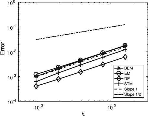
In Figure 2, we illustrate numerically the strong rate of convergence of the drift-preserving scheme (5(5) $\begin{array}{rl}{Y}_1& :=X_n+\left(\begin{array}{c}\mathrm{\Sigma }\\ 0\end{array}\right)(W(t_n+\frac{h}{2})-W(t_n)),\\ Y_2& :=Y_1+hB\left(\frac{Y_1+Y_2}{2}\right){\int }_0^1\mathrm{\nabla }H(Y_1+\theta (Y_2-Y_1))\mathrm{d}\theta ,\\ X_{n+1}& =Y_2+\left(\begin{array}{c}\mathrm{\Sigma }\\ 0\end{array}\right)(W(t_{n+1})-W(t_n+\frac{h}{2})).\end{array}$(5) ) and compare with the other schemes. To this aim, we discretize the linear stochastic oscillator on the time interval $[0,1]$ using step sizes ranging from $h=2^{-6}$ to $h=2^{-10}$ and we use as a reference solution the stochastic trigonometric method with small time step $h_{\mathrm{ref}}=2^{-12}$. The expected values are approximated by computing averages over $M={10}^6$ samples. One can observe the mean-square order 1 of convergence of the drift-preserving scheme (5(5) $\begin{array}{rl}{Y}_1& :=X_n+\left(\begin{array}{c}\mathrm{\Sigma }\\ 0\end{array}\right)(W(t_n+\frac{h}{2})-W(t_n)),\\ Y_2& :=Y_1+hB\left(\frac{Y_1+Y_2}{2}\right){\int }_0^1\mathrm{\nabla }H(Y_1+\theta (Y_2-Y_1))\mathrm{d}\theta ,\\ X_{n+1}& =Y_2+\left(\begin{array}{c}\mathrm{\Sigma }\\ 0\end{array}\right)(W(t_{n+1})-W(t_n+\frac{h}{2})).\end{array}$(5) ) with lines of slope 1 in Figure 2, which corroborates Theorem 3.1.

Figure 2. Linear stochastic oscillator: mean-square convergence rates for the backward Euler–Maruyama scheme (BEM), the Euler–Maruyama scheme (EM), the drift-preserving scheme (DP), and the stochastic trigonometric method (STM). Reference lines of slopes 1, resp. 1/2.

Next, Figure 3 illustrates the weak convergence rate of the drift-preserving scheme (5(5) $\begin{array}{rl}{Y}_1& :=X_n+\left(\begin{array}{c}\mathrm{\Sigma }\\ 0\end{array}\right)(W(t_n+\frac{h}{2})-W(t_n)),\\ Y_2& :=Y_1+hB\left(\frac{Y_1+Y_2}{2}\right){\int }_0^1\mathrm{\nabla }H(Y_1+\theta (Y_2-Y_1))\mathrm{d}\theta ,\\ X_{n+1}& =Y_2+\left(\begin{array}{c}\mathrm{\Sigma }\\ 0\end{array}\right)(W(t_{n+1})-W(t_n+\frac{h}{2})).\end{array}$(5) ). For simplicity, we only display the errors in the first and second moments since explicit formulas are available for these quantities. We take the noise scaling parameter $\mathrm{\Sigma }=0.1$ and step sizes ranging from $h=2^{-4}$ to $h=2^{-16}$. The remaining parameters are the same as in the previous numerical experiment. The lines of slope 2 in Figure 3 illustrates that the drift-preserving scheme has a weak order of convergence 2 in the first and second moments, as stated in Theorem 3.2.

Figure 3. Linear stochastic oscillator: weak convergence rates for the backward Euler–Maruyama scheme (BEM), the Euler–Maruyama scheme (EM), the drift-preserving scheme (DP), and the stochastic trigonometric method (STM). Reference lines of slopes 1, resp. 2. (a) Errors in the first moments $\mathbb{E}[q(t)]$ (left) and $\mathbb{E}[p(t)]$ (right), (b) Errors in the second moments $\mathbb{E}[q(t{)}^2]$ (left) and $\mathbb{E}[p(t{)}^2]$ (right).

As symplectic integrators for deterministic Hamiltonian systems have proven to be very successful [25], it may be tempting to use them in a splitting scheme for the SDE (2(2) $\mathrm{d}X(t)=B(X(t))\mathrm{\nabla }H(X(t))\mathrm{d}t+\left(\begin{array}{c}\mathrm{\Sigma }\\ 0\end{array}\right)\mathrm{d}W(t).$(2) ). To study this, in Figure 4, we compare the behaviour, with respect to the trace formula, of the drift-preserving scheme and of the symplectic splitting strategies discussed in Section 2.4. We use the classical Euler symplectic and Störmer–Verlet schemes for the deterministic Hamiltonian and integrate the noisy part exactly. These numerical integrators are denoted by SYMP, resp. ST below. As a comparison with non-geometric numerical integrators, we also use the classical Euler and Heun's schemes in place of a symplectic scheme. These numerical integrators are denoted by splitEULER and splitHEUN. We discretize the linear stochastic oscillator on the time interval $[0,100]$ with $2^7$ step sizes. It can be observed that the splitting method using the non-symplectic schemes splitEULER or splitHEUN behaves as poorly as standard explicit schemes for SDEs: we hence display in Figure 4 only part of their numerical values due to their exponential growth. Although not having the exact growth rates, the two symplectic splitting schemes behave much better than the classical Euler–Maruyama scheme with a linear drift in the averaged energy with a perturbed rate, as predicted by Proposition 2.3.

Figure 4. Linear stochastic oscillator: numerical trace formulas for $\mathbb{E}[H(p(t),q(t))]$ on the interval $[0,100]$. Comparison of the drift-preserving scheme (DP), the splitting methods with, respectively, the symplectic Euler method (SYMP), the Störmer-Verlet method (ST), the explicit Euler method (splitEULER), the Heun method (splitHEUN), and the exact solution.

4.2. The stochastic mathematical pendulum

Let us next consider the nonlinear SDE (2(2) $\mathrm{d}X(t)=B(X(t))\mathrm{\nabla }H(X(t))\mathrm{d}t+\left(\begin{array}{c}\mathrm{\Sigma }\\ 0\end{array}\right)\mathrm{d}W(t).$(2) ) (with $B(X)=J$ the constant canonical Poisson matrix) with the Hamiltonian $H(p,q)=\frac{1}{2}{p}^2-\cos (q)$and a noise in dimension one with parameter $\mathrm{\Sigma }=1$. We take the initial values $(p_0,q_0)=(1,\sqrt{2})$.

We again compare the behaviour, with respect to the trace formula, of the DP, SYMP, ST and splitEULER schemes. To do this, we integrate numerically the stochastic mathematical pendulum on the time interval $[0,100]$ with $2^7$ step sizes. The results are presented in Figure 5. Again, we recover the fact that the drift-preserving scheme exhibits the exact averaged energy drift, as predicted in Theorem 2.2. Furthermore, one can still observe a good behaviour of the symplectic strategies from Section 2.4 analogously to the linear case in Section 4.1, although the analysis in Proposition 2.3 is only valid for the linear case.

Figure 5. Stochastic mathematical pendulum: numerical trace formulas for $\mathbb{E}[H(p(t),q(t))]$ on the interval $[0,100]$. Comparison of the drift-preserving scheme (DP), the splitting methods with, respectively, the symplectic Euler method (SYMP), the Störmer-Verlet method (ST), the explicit Euler method (splitEULER), and the exact solution.

4.3. Stochastic rigid body problem

We now consider an Itô version of the stochastic rigid body problem studied in [1,16,33] for instance. This system has the following Hamiltonian: $H(X)=\frac{1}{2}(X_1^2/I_1+X_2^2/I_2+X_3^2/I_3),$the quadratic Casimir $C(X)=\frac{1}{2}(X_1^2+X_2^2+X_3^2),$and the skew-symmetric matrix $B(X)=\left(\begin{array}{ccc}0& -X_3& X_2\\ X_3& 0& -X_1\\ -X_2& X_1& 0\end{array}\right).$ Here, we denote the angular momentum by $X=(X_1,X_2,X_3{)}^{\mathrm{\top }}$ and take the moments of inertia to be $I=(I_1,I_2,I_3)=(0.345,0.653,1)$. The initial value for the SDE (2(2) $\mathrm{d}X(t)=B(X(t))\mathrm{\nabla }H(X(t))\mathrm{d}t+\left(\begin{array}{c}\mathrm{\Sigma }\\ 0\end{array}\right)\mathrm{d}W(t).$(2) ) is given by $X(0)=(0.8,0.6,0)$ and we consider a scalar noise $W(t)$ with $\mathrm{\Sigma }=0.25$ (acting on the first component $X_1$ only).

Observe that, even if the Hamiltonian has not the desired structure (1(1) $H(p,q)=\frac{1}{2}\sum _{j=1}^m{p}_j^2+V(q).$(1) ), one still has a linear drift in the energy since the Hamiltonian is quadratic and thus the Hessian matrix present in the derivation of the trace formula has the correct structure as noted in Remark 2.1.

In Figure 6, we compute the expected values of the energy $H(X)$ and the Casimir $C(X)$ using $N=2^5$ step sizes on the time interval $[0,4]$ (in order to see also the behaviour of the Euler–Maruyama scheme) along various numerical solutions. The expected values are approximated by computing averages over $M={10}^6$ samples. The exact long-time behaviour with respect to the energy and the Casimir averaged growths of the drift-preserving scheme can be observed in Figure 6, which corroborates Theorem 2.2 and Proposition 2.4. As in the previous numerical experiment, one can also see that the growth rates of the Euler–Maruyama schemes are in contrast qualitatively wrong.

Figure 6. Stochastic rigid body problem: numerical trace formulas for the energy $\mathbb{E}[H(X(t))]$ (left) and for the Casimir $\mathbb{E}[C(X(t))]$ (right) for the drift-preserving scheme (DP), the Euler–Maruyama scheme (EM), the backward Euler–Maruyama scheme (BEM), and the exact solution.

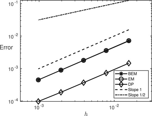
Similarly to the previous example, we numerically illustrate in Figure 7 the strong convergence rate of the drift-preservation scheme (5(5) $\begin{array}{rl}{Y}_1& :=X_n+\left(\begin{array}{c}\mathrm{\Sigma }\\ 0\end{array}\right)(W(t_n+\frac{h}{2})-W(t_n)),\\ Y_2& :=Y_1+hB\left(\frac{Y_1+Y_2}{2}\right){\int }_0^1\mathrm{\nabla }H(Y_1+\theta (Y_2-Y_1))\mathrm{d}\theta ,\\ X_{n+1}& =Y_2+\left(\begin{array}{c}\mathrm{\Sigma }\\ 0\end{array}\right)(W(t_{n+1})-W(t_n+\frac{h}{2})).\end{array}$(5) ) for the stochastic rigid body problem. To this aim, we discretize the problem on the time interval $[0,0.75]$ using step sizes ranging from $h=2^{-6}$ to $h=2^{-10}$ and compare with a reference solution obtained with scheme (5(5) $\begin{array}{rl}{Y}_1& :=X_n+\left(\begin{array}{c}\mathrm{\Sigma }\\ 0\end{array}\right)(W(t_n+\frac{h}{2})-W(t_n)),\\ Y_2& :=Y_1+hB\left(\frac{Y_1+Y_2}{2}\right){\int }_0^1\mathrm{\nabla }H(Y_1+\theta (Y_2-Y_1))\mathrm{d}\theta ,\\ X_{n+1}& =Y_2+\left(\begin{array}{c}\mathrm{\Sigma }\\ 0\end{array}\right)(W(t_{n+1})-W(t_n+\frac{h}{2})).\end{array}$(5) ) with $h_{\mathrm{ref}}=2^{-12}$. We compute averages over $M={10}^5$ samples to approximate the expected values present in the mean-square errors. One observes again mean-square convergence of order 1 for the drift-preserving scheme.

Figure 7. Stochastic rigid body problem: mean-square convergence rates for the backward Euler–Maruyama scheme (BEM), the drift-preserving scheme (DP), and the Euler–Maruyama scheme (EM). Reference lines of slopes 1, resp. 1/2.

Next, Figure 8 illustrates the weak convergence rate of the drift-preserving scheme (5(5) $\begin{array}{rl}{Y}_1& :=X_n+\left(\begin{array}{c}\mathrm{\Sigma }\\ 0\end{array}\right)(W(t_n+\frac{h}{2})-W(t_n)),\\ Y_2& :=Y_1+hB\left(\frac{Y_1+Y_2}{2}\right){\int }_0^1\mathrm{\nabla }H(Y_1+\theta (Y_2-Y_1))\mathrm{d}\theta ,\\ X_{n+1}& =Y_2+\left(\begin{array}{c}\mathrm{\Sigma }\\ 0\end{array}\right)(W(t_{n+1})-W(t_n+\frac{h}{2})).\end{array}$(5) ). We plot the weak errors in the first and second moments of the first component of the solutions using the parameters: $\mathrm{\Sigma }=0.1$, T = 1, M = 2500 samples, and step sizes ranging from $h=2^{-10}$ to $h=2^{-20}$. The rest of the parameters are as in the previous numerical experiment. One can observe weak order 2 in the first and second moments for the drift-preserving scheme (up to Monte Carlo errors), which confirms again the statement of Theorem 3.2.

Figure 8. Stochastic rigid body problem: weak convergence rates in the first moment $\mathbb{E}[X_1(t_n)]$ (left) and second moment $\mathbb{E}[X_1(t_n{)}^2]$ (right) for the drift-preserving scheme (DP), the Euler–Maruyama scheme (EM), and the backward Euler–Maruyama scheme (BEM). Reference lines of slopes 1, resp. 2.

Finally, in Figure 9, we take the same parameters as in the first experiment of this subsection but we consider a noise in dimension two with the matrix $\mathrm{\Sigma }=\left(\begin{array}{cc}0.25& 0\\ 0& 0.25\end{array}\right).$We then compute the expected values of the energy $H(X)$ and the Casimir $C(X)$ using $N=2^6$ step sizes along various numerical solutions and display the trace formula for the energy $\mathbb{E}[H(X(t))]=\mathbb{E}[H(X_0)]+\frac{1}{2}\mathrm{Tr}\left({\mathrm{\Sigma }}^{\mathrm{\top }}\left(\begin{array}{cc}1/I_1& 0\\ 0& 1/I_2\end{array}\right)\mathrm{\Sigma }\right)t$and the trace formula for the Casimir $\mathbb{E}[C(X(t))]=\mathbb{E}[C(X_0)]+\frac{1}{2}\mathrm{Tr}\left({\mathrm{\Sigma }}^{\mathrm{\top }}\mathrm{\Sigma }\right)t.$Again, one can observe in Figure 9 the excellent behaviour of the drift-preserving scheme as stated in Theorem 2.2 and Proposition 2.4.

Figure 9. Stochastic rigid body problem with two-dimensional noise: numerical trace formulas for the energy $\mathbb{E}[H(X(t))]$ (left) and for the Casimir $\mathbb{E}[C(X(t))]$ (right) for the Casimir $\mathbb{E}[C(X(t))]$ (right) for the drift-preserving scheme (DP), the Euler–Maruyama scheme (EM), the backward Euler–Maruyama scheme (BEM), and the exact solution.

Acknowledgements

We appreciate the referees' comments on an earlier version of the paper.

Disclosure statement

No potential conflict of interest was reported by the author(s).

Additional information

Funding

The work of DC was supported by the Swedish Research Council (VR) (projects nr. 2018−04443). The work of GV was partially supported by the Swiss National Science Foundation, grants No. 200020_184614, No. 200021_162404 and No. 200020_178752. The computations were performed on resources provided by the Swedish National Infrastructure for Computing (SNIC) at HPC2N, Umeå University and UPPMAX, Uppsala University.

References

- A. Abdulle, D. Cohen, G. Vilmart, and K. Zygalakis, High order weak methods for stochastic differential equations based on modified equations, SIAM J. Sci. Comput. 34 (2012), pp. A1800–A1823. Available at https://doi.org/https://doi.org/10.1137/110846609.
- A. Alamo and J.M. Sanz-Serna, Word combinatorics for stochastic differential equations: splitting integrators, Commun. Pure Appl. Anal. 18 (2019), pp. 2163–2195. MR 3927434.
- R. Anton and D. Cohen, Exponential integrators for stochastic Schrödinger equations driven by itønoise, J. Comput. Math. 36 (2018), pp. 276–309. Available at https://doi.org/https://doi.org/10.4208/jcm.1701-m2016-0525 MR 3771721.
- R. Anton, D. Cohen, S. Larsson, and X. Wang, Full discretization of semilinear stochastic wave equations driven by multiplicative noise, SIAM J. Numer. Anal. 54 (2016), pp. 1093–1119. Available at https://doi.org/https://doi.org/10.1137/15M101049X. MR 3484400.
- S. Blanes and F. Casas, A concise introduction to geometric numerical integration, Monographs and Research Notes in Mathematics, CRC Press, Boca Raton, FL, 2016. MR 3642447.
- L. Brugnano, M. Calvo, J.I. Montijano, and L. Rández, Energy-preserving methods for Poisson systems, J. Comput. Appl. Math. 236 (2012), pp. 3890–3904. Available at https://doi.org/https://doi.org/10.1016/j.cam.2012.02.033. MR 2926249.
- L. Brugnano, G. Gurioli, and F. Iavernaro, Analysis of energy and quadratic invariant preserving (EQUIP) methods, J. Comput. Appl. Math. 335 (2018), pp. 51–73. Available at https://doi.org/https://doi.org/10.1016/j.cam.2017.11.043. MR 3758633.
- L. Brugnano and F. Iavernaro, Line integral methods which preserve all invariants of conservative problems, J. Comput. Appl. Math. 236 (2012), pp. 3905–3919. Available at https://doi.org/https://doi.org/10.1016/j.cam.2012.03.026. MR 2926250.
- P.M. Burrage and K. Burrage, Structure-preserving Runge–Kutta methods for stochastic Hamiltonian equations with additive noise, Numer. Algor. 65 (2014), pp. 519–532. Available at https://doi.org/https://doi.org/10.1007/s11075-013-9796-6. MR 3172331.
- E. Celledoni, M. Farré Puiggalí, E.H. Høiseth, and D. Martín de Diego, Energy-preserving integrators applied to nonholonomic systems, J. Nonlinear Sci. 29 (2019), pp. 1523–1562. Available at https://doi.org/https://doi.org/10.1007/s00332-018-9524-4. MR 3993177.
- E. Celledoni, R.I. McLachlan, D.I. McLaren, B. Owren, G.R.W. Quispel, and W.M. Wright, Energy-preserving Runge–Kutta methods, M2AN Math. Model. Numer. Anal. 43 (2009), pp. 645–649. Available at https://doi.org/https://doi.org/10.1051/m2an/2009020. MR 2542869.
- E. Celledoni, B. Owren, and Y. Sun, The minimal stage, energy preserving Runge–Kutta method for polynomial Hamiltonian systems is the averaged vector field method, Math. Comput. 83 (2014), pp. 1689–1700. Available at https://doi.org/https://doi.org/10.1090/S0025-5718-2014-02805-6. MR 3194126.
- C. Chen, D. Cohen, R. D'Ambrosio, and A. Lang, Drift-preserving numerical integrators for stochastic Hamiltonian systems, Adv. Comput. Math. 46 (2020), pp. 1–22. Available at https://doi.org/https://doi.org/10.1007/s10444-020-09771-5.
- D. Cohen, On the numerical discretisation of stochastic oscillators, Math. Comput. Simul. 82 (2012), pp. 1478–1495. Available at https://doi.org/https://doi.org/10.1016/j.matcom.2012.02.004. MR 2922170.
- D. Cohen, J. Cui, J. Hong, and L. Sun, Exponential integrators for stochastic Maxwell's equations driven by itô noise, J. Comput. Phys. 410 (2020), pp. 109382.Available at http://www.sciencedirect.com/science/article/pii/S0021999-12030156X.
- D. Cohen and G. Dujardin, Energy-preserving integrators for stochastic Poisson systems, Commun. Math. Sci. 12 (2014), pp. 1523–1539. Available at https://doi.org/https://doi.org/10.4310/CMS.2014.v12.n8.a7. MR 3210739.
- D. Cohen and E. Hairer, Linear energy-preserving integrators for Poisson systems, BIT 51 (2011), pp. 91–101. Available at https://doi.org/https://doi.org/10.1007/s10543-011-0310-z. MR 2784654.
- D. Cohen, S. Larsson, and M. Sigg, A trigonometric method for the linear stochastic wave equation, SIAM J. Numer. Anal. 51 (2013), pp. 204–222. Available at https://doi.org/https://doi.org/10.1137/12087030X. MR 3033008.
- D. Cohen and M. Sigg, Convergence analysis of trigonometric methods for stiff second-order stochastic differential equations, Numer. Math. 121 (2012), pp. 1–29. Available at https://doi.org/https://doi.org/10.1007/s00211-011-0426-8. MR 2909913.
- J. Cui, J. Hong, and D. Sheng, Convergence in density of splitting AVF scheme for stochastic Langevin equation, arXiv (2019) Available at https://arxiv.org/abs/1906.03439.
- H. de la Cruz, J.C. Jimenez, and J.P. Zubelli, Locally linearized methods for the simulation of stochastic oscillators driven by random forces, BIT 57 (2017), pp. 123–151. Available at https://doi.org/https://doi.org/10.1007/s10543-016-0620-2. MR 3608313.
- O. Gonzalez, Time integration and discrete Hamiltonian systems, J. Nonlinear Sci. 6 (1996), pp. 449–467. Available at https://doi.org/https://doi.org/10.1007/s003329900018. MR 1411343.
- E. Hairer, Energy-preserving variant of collocation methods, JNAIAM. J. Numer. Anal. Ind. Appl. Math. 5 (2010), pp. 73–84. MR 2833602.
- E. Hairer, C. Lubich, and G. Wanner, Geometric numerical integration illustrated by the Störmer–Verlet method, Acta Numer.12 (2003), pp. 399–450. Available at https://doi.org/https://doi.org/10.1017/S0962492902000144. MR 2249159.
- E. Hairer, C. Lubich, and G. Wanner, Geometric Numerical Integration: Structure-Preserving Algorithms for Ordinary Differential Equations, 2nd ed., Springer-Verlag, Berlin, Heidelberg, 2006.
- M. Han, Q. Ma, and X. Ding, High-order stochastic symplectic partitioned Runge–Kutta methods for stochastic Hamiltonian systems with additive noise, Appl. Math. Comput. 346 (2019), pp. 575–593. Available at https://doi.org/https://doi.org/10.1016/j.amc.2018.10.041. MR 3873562.
- D.D. Holm and T.M. Tyranowski, Stochastic discrete Hamiltonian variational integrators, BIT 58 (2018), pp. 1009–1048. Available at https://doi.org/https://doi.org/10.1007/s10543-018-0720-2. MR 3882980.
- J. Hong, R. Scherer, and L. Wang, Midpoint rule for a linear stochastic oscillator with additive noise, Neural Parallel Sci. Comput. 14 (2006), pp. 1–12. MR 2359504.
- F. Iavernaro and D. Trigiante, High-order symmetric schemes for the energy conservation of polynomial Hamiltonian problems, JNAIAM J. Numer. Anal. Ind. Appl. Math. 4 (2009), pp. 87–101. MR 2598786.
- H. Kojima, Invariants preserving schemes based on explicit Runge–Kutta methods, BIT 56 (2016), pp. 1317–1337. Available at https://doi.org/https://doi.org/10.1007/s10543-016-0608-y. MR 3576613.
- Y. Komori, D. Cohen, and K. Burrage, Weak second order explicit exponential Runge–Kutta methods for stochastic differential equations, SIAM J. Sci. Comput. 39 (2017), pp. A2857–A2878. Available at https://doi-org.proxy.ub.umu.se/https://doi.org/10.1137/15M1041341. MR 3735294.
- B. Leimkuhler and S. Reich. Simulating Hamiltonian dynamics, Cambridge Monographs on Applied and Computational Mathematics Vol. 14, Cambridge University Press, Cambridge, 2004. MR 2132573.
- M. Liao, Random motion of a rigid body, J. Theor. Probab. 10 (1997), pp. 201–211. Available at https://doi-org.proxy.ub.umu.se/https://doi.org/10.1023/A:1022654717555. MR 1432623.
- R.I. McLachlan, G.R.W. Quispel, and N. Robidoux, Geometric integration using discrete gradients, R. Soc. Lond. Philos. Trans. Ser. A Math. Phys. Eng. Sci. 357 (1999), pp. 1021–1045. Available at https://doi.org/https://doi.org/10.1098/rsta.1999.0363. MR 1694701.
- G.N. Milstein, Y.M. Repin, and M.V. Tretyakov, Symplectic integration of Hamiltonian systems with additive noise, SIAM J. Numer. Anal. 39 (2002), pp. 2066–2088. Available at https://doi-org.proxy.ub.umu.se/https://doi.org/10.1137/S0036142-901387440. MR 1897950.
- G.N. Milstein and M.V. Tretyakov, Stochastic Numerics for Mathematical Physics, Scientific Computation, Springer-Verlag, Berlin, 2004. Available at https://doi.org/https://doi.org/10.1007/978-3-662-10063-9. MR 2069903.
- Y. Miyatake, An energy-preserving exponentially-fitted continuous stage Runge–Kutta method for Hamiltonian systems, BIT 54 (2014), pp. 777–799. Available at https://doi.org/https://doi.org/10.1007/s10543-014-0474-4. MR 3259826.
- Y. Miyatake and J.C. Butcher, A characterization of energy-preserving methods and the construction of parallel integrators for Hamiltonian systems, SIAM J. Numer. Anal. 54 (2016), pp. 1993–2013. Available at https://doi.org/https://doi.org/10.1137/15M1020861. MR 3516866.
- G.R.W. Quispel and D.I. McLaren, A new class of energy-preserving numerical integration methods, J. Phys. A 41 (2008), pp. 045206.
- J.M. Sanz-Serna and M.P. Calvo, Numerical Hamiltonian problems, Applied Mathematics and Mathematical Computation Vol. 7, Chapman & Hall, London, 1994. MR 1270017.
- H. Schurz, Analysis and discretization of semi-linear stochastic wave equations with cubic nonlinearity and additive space-time noise, Discr Contin. Dyn. Syst. Ser. S 1 (2008), pp. 353–363. Available at https://doi.org/https://doi.org/10.3934/dcdss.2008.1.353. MR 2379913.
- M. Seesselberg, H.P. Breuer, F. Petruccione, J. Honerkamp, and H. Mais, Simulation of one-dimensional noisy hamiltonian systems and their application to particle storage rings, Z. Phys.C62 (1994), pp. 63–73.
- M.J. Senosiain and A. Tocino, A review on numerical schemes for solving a linear stochastic oscillator, BIT 55 (2015), pp. 515–529. Available at https://doi.org/https://doi.org/10.1007/s10543-014-0507-z. MR 3348201.
- A.H. Strømmen Melbø and D.J. Higham, Numerical simulation of a linear stochastic oscillator with additive noise, Appl. Numer. Math. 51 (2004), pp. 89–99. Available at https://doi.org/https://doi.org/10.1016/j.apnum.2004.02.003. MR 2083326.
- N. Tasaka, S. Satoh, T. Hatanaka, and K. Yamada, Stochastic stabilization of rigid body motion of a spacecraft on SE(3), Int. J. Control. 94 (2021), pp. 1–8. Available at https://doi.org/https://doi.org/10.1080/00207179.2019.1637544.
- G. Vilmart, Weak second order multirevolution composition methods for highly oscillatory stochastic differential equations with additive or multiplicative noise, SIAM J. Sci. Comput. 36 (2014), pp. A1770–A1796. Available at https://doi-org.proxy.ub.umu.se/https://doi.org/10.1137/130935331. MR 3246903.
- J. Walter, O. Gonzalez, and J.H. Maddocks, On the stochastic modeling of rigid body systems with application to polymer dynamics, Multiscale Model. Simul. 8 (2010), pp. 1018–1053. Available at https://doi.org/https://doi.org/10.1137/090765705. MR 2644322.
- B. Wang and X. Wu, Functionally-fitted energy-preserving integrators for Poisson systems, J. Comput. Phys. 364 (2018), pp. 137–152. Available at https://doi.org/https://doi.org/10.1016/j.jcp.2018.03.015. MR 3787423.
- X. Wu, B. Wang, and W. Shi, Efficient energy-preserving integrators for oscillatory Hamiltonian systems, J. Comput. Phys. 235 (2013), pp. 587–605. Available at https://doi.org/https://doi.org/10.1016/j.jcp.2012.10.015. MR 3017613.
- W. Zhou, J. Zhang, J. Hong, and S. Song, Stochastic symplectic Runge–Kutta methods for the strong approximation of Hamiltonian systems with additive noise, J. Comput. Appl. Math. 325 (2017), pp. 134–148. Available at https://doi.org/https://doi.org/10.1016/j.cam.2017.04.050. MR 3658901.