Stable inversion of LPTV systems with application in position-dependent and non-equidistantly sampled systems

ABSTRACT

Many control applications, including feedforward and learning control, involve the inverse of a dynamical system. For nonminimum-phase systems, the response of the inverse system is unbounded. For linear time-invariant (LTI), nonminimum-phase systems, a bounded, noncausal inverse response can be obtained through an exponential dichotomy. For generic linear time-varying (LTV) systems, such a dichotomy does not exist in general. The aim of this paper is to develop an inversion approach for an important class of LTV systems, namely linear periodically time-varying (LPTV) systems, which occur in, e.g. position-dependent systems with periodic tasks and non-equidistantly sampled systems. The proposed methodology exploits the periodicity to determine a bounded inverse for general LPTV systems. Conditions for existence are provided. The method is successfully demonstrated in several application cases, including position-dependent and non-equidistantly sampled systems.

KEYWORDS:

• Stable inversion
• dichotomy
• linear time-varying systems
• linear periodically time-varying systems
• tracking control

1. Introduction

Inverses of dynamical systems are essential in many control applications, including feedforward and learning control. The early inversion approaches in Silverman (1969) and Hirschorn (1979) are restricted to causal inverses of minimum-phase systems since they lead to unbounded responses for nonminimum-phase systems. See, for example, Butterworth, Pao, and Abramovitch (2008) for the effect of nonminimum-phase zeros. Interestingly, in Devasia and Paden (1994), Hunt, Meyer, and Su (1996) and Devasia, Chen, and Paden (1996), an exact inverse for nonminimum-phase systems is obtained with bounded responses. This stable inversion approach is based on a dichotomy of the inverted system into a stable part and an unstable part. It essentially uses a bilateral Laplace or Z-transform (Sogo, 2010) by regarding the unstable part as an anti-causal operation and solving it backward in time. For linear time-invariant (LTI) systems, such a dichotomy is trivial and successful applications in feedforward and learning control are reported in Boeren, Oomen, and Steinbuch (2015), Bolder and Oomen (2015) and Clayton, Tien, Leang, Zou, and Devasia (2009).

Linear time variance has a large impact on system inversion approaches. Such linear time-varying (LTV) applications occur frequently, e.g. (i) multirate systems with different sampling frequencies (Chen & Francis, 1995; Fujimoto & Hori, 2002; Ohnishi & Fujimoto, 2016); (ii) non-equidistantly sampled systems with time-varying sampling intervals (van Zundert et al. 2016); and (iii) position-dependent systems with periodic tasks (van Zundert et al. 2016). Similar to LTI systems, direct inversion of LTV systems can lead to unbounded responses if a causal inverse is computed. For these applications, it is of direct interest to compute system inverses with bounded responses, similar to stable inversion techniques for LTI systems. However, an exponential dichotomy for LTV systems is non-trivial. In fact, such a dichotomy does not exist for the general class of LTV systems, as is shown in Coppel (1978) and Section 3 of this paper.

Although stable inversion is a standard technique for LTI systems, it does not directly apply to LTV systems. The aim of this paper is to provide a direct solution for linear periodically time-varying (LPTV) systems, which form an important subclass of LTV systems. In fact, the mentioned LTV applications (i)--(iii) typically satisfy the additional periodicity property. In this paper, the periodicity of LPTV systems is exploited to establish the required exponential dichotomy, enabling the use of stable inversion for LPTV systems. The presented work relates to Devasia and Paden (1994), Hunt et al. (1996), Devasia et al. (1996), Devasia and Paden (1998) and Pavlov and Pettersen (2008) where nonlinear systems are investigated and related conditions are imposed on the system, and to Devasia and Paden (1998), Zou and Devasia (1999), Zou and Devasia (2004), Zou (2009) and Jetto, Orsini, and Romagnoli (2015) where perfect tracking is compromised for finite preview, with extension to nonlinear systems in Zou and Devasia (2007). For LTI systems, approaches related to stable inversion include inversion via lifting (Bayard, 1994), geometric approaches (Marro, Prattichizzo, & Zattoni, 2002; Zattoni, 2014), and state-space reduction for non-square systems (Moylan, 1977).

The main contribution of this paper is stable inversion for LPTV systems, with the following sub-contributions: (I) it is shown that an exponential dichotomy does not always exist for general LTV systems; (II) it is shown that an exponential dichotomy always exists for LPTV systems under mild conditions similar to those for LTI systems; (III) two computational procedures of the exponential dichotomy for LPTV systems are provided: one for reversible systems and one for non-reversible systems; (IV) the proposed approach is demonstrated via three cases: (i) a reversible numerical example; (ii) a non-equidistantly sampled system; and (iii) a position-dependent system. Preliminary results are reported in van Zundert and Oomen (2017). The present paper extends those by contributions (I), (III), and (IV).

The outline is as follows. In Section 2, the stable inversion problem for general LTV systems is formulated. The key issue lies in finding an exponential dichotomy. In Section 3, it is shown that such a dichotomy does not always exist for general LTV systems. In Section 4, the exponential dichotomy for LPTV systems is presented and shown to always exist. In Section 5, the stable inversion approach for LPTV systems is presented. The approach is demonstrated using several cases in Sections 6–Section 8. Section 9 contains conclusions.

Throughout, linear, single-input, single-output (SISO) systems are considered. Extensions to multi-input, multi-output (MIMO) systems follow directly. The focus is on discrete-time systems, since this is natural for sampled systems. Results for continuous-time systems follow along similar lines.

2. Problem formulation

2.1 Application in mechatronics

In mechatronics, there is an ever increasing demand for lower cost and higher accuracy, introducing LPTV behaviour. At least three cases causing this behaviour can be identified: (i) multirate systems, (ii) non-equidistant sampling, and (iii) position-dependent behaviour with periodic tasks. These cases are detailed below.

To reduce cost, multiple applications are often embedded on a single platform. Scheduling of the different processes leads to non-equidistant sampling of the applications, which is observed as time-variance of the system (see Figure 1(a)). The scheduling is often periodic, leading to LPTV behaviour. LTI control design for a lower equidistant rate is conservative in terms of performance since not all design freedom is exploited. To enhance the performance/cost trade-off, control design of the LPTV system is desired.

Figure 1. LPTV behaviour occurs in many mechatronic applications.

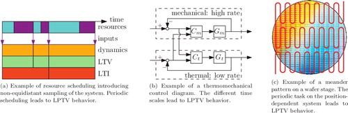
To reduce cost, the applications can also run on different dedicated control boards, depending on the performance requirement of the specific (control) loop. For example, fast dynamics are typically controlled with a higher sampling rate than slow dynamics, as is, for example, the case in thermomechanical systems (see Figure 1(b)). The interconnection of the different loops forms a multirate system with LPTV behaviour.

Accuracy is often limited by the inherent position-dependent behaviour of mechatronic systems. However, most control is based on LTI designs, not taking into account the position-dependent behaviour. For periodic motion tasks, as for example in Figure 1(c), the position-dependent behaviour leads to LPTV behaviour. Taking the LPTV behaviour into account for control design can significantly improve the accuracy.

2.2 Problem setup

Consider the exponentially stable LTV system H: (1a) $$x_{k+1}=A_k^H{x}_k+B_k^H{u}_k,$$(1a) (1b) $$y_k=C_k^H{x}_k+D_k^H{u}_k,$$(1b) where $A_k^H\in {\mathbb{R}}^{n_x\times n_x}$, $B_k^H\in {\mathbb{R}}^{n_x\times 1}$, $C_k^H\in {\mathbb{R}}^{1\times n_x}$, $D_k^H\in \mathbb{R}$, with time index k, k _s ≤ k ≤ k _e , $k_s,k,k_e\in \mathbb{Z}$, and $z_{k_s}=0$.

The considered problem in this paper is to determine a bounded input u, such that y = r in Figure 2. In particular, the main idea is to invert the system H, i.e. for square and invertible H use (2) $$\begin{array}{c}\hfill F\stackrel{s}{=}\left[\begin{array}{cc}{A}_k& B_k\\ C_k& D_k\end{array}\right]=\left[\begin{array}{cc}{A}_k^H-B_k^H{\left(D_k^H\right)}^{-1}{C}_k^H& B_k^H{\left(D_k^H\right)}^{-1}\\ -{\left(D_k^H\right)}^{-1}{C}_k^H& {\left(D_k^H\right)}^{-1}\end{array}\right].\end{array}$$(2) The main point is that F in (2(2) $$\begin{array}{c}\hfill F\stackrel{s}{=}\left[\begin{array}{cc}{A}_k& B_k\\ C_k& D_k\end{array}\right]=\left[\begin{array}{cc}{A}_k^H-B_k^H{\left(D_k^H\right)}^{-1}{C}_k^H& B_k^H{\left(D_k^H\right)}^{-1}\\ -{\left(D_k^H\right)}^{-1}{C}_k^H& {\left(D_k^H\right)}^{-1}\end{array}\right].\end{array}$$(2) ) need not be exponentially stable. The zeros of (1) can be immediately verified to be eigenvalues of A^H _k − B^H _k (D^H _k )^{− 1} C^H _k , which in fact are the poles of (2(2) $$\begin{array}{c}\hfill F\stackrel{s}{=}\left[\begin{array}{cc}{A}_k& B_k\\ C_k& D_k\end{array}\right]=\left[\begin{array}{cc}{A}_k^H-B_k^H{\left(D_k^H\right)}^{-1}{C}_k^H& B_k^H{\left(D_k^H\right)}^{-1}\\ -{\left(D_k^H\right)}^{-1}{C}_k^H& {\left(D_k^H\right)}^{-1}\end{array}\right].\end{array}$$(2) ). Hence, stability of F in (2(2) $$\begin{array}{c}\hfill F\stackrel{s}{=}\left[\begin{array}{cc}{A}_k& B_k\\ C_k& D_k\end{array}\right]=\left[\begin{array}{cc}{A}_k^H-B_k^H{\left(D_k^H\right)}^{-1}{C}_k^H& B_k^H{\left(D_k^H\right)}^{-1}\\ -{\left(D_k^H\right)}^{-1}{C}_k^H& {\left(D_k^H\right)}^{-1}\end{array}\right].\end{array}$$(2) ) hinges on the zeros of H in (1). More on zero dynamics and stability of LTV systems can be found in, for example, Hill and Ilchmann (2011) and Berger, Ilchmann, and Wirth (2015).

Figure 2. For nonminimum-phase system H, stable inversion yields bounded signal u such that y = r.

The following definition is adopted from Coppel (1978), Halanay and Ionescu (1994) and Papaschinopoulos (1986).

Definition 2.1 (Exponential dichotomy):

The system (3) $$\begin{array}{c}\hfill x_{k+1}=A_k{x}_k,\end{array}$$(3) with $A_k\in {\mathbb{R}}^{n_x\times n_x}$ and fundamental matrix solution $X_k\in {\mathbb{R}}^{n_x\times n_x}$ satisfies an exponential dichotomy if there exist a projection $P=P^2\in {\mathbb{R}}^{n_x\times n_x}$ and constants K > 0, 0 < p < 1 such that (4a) $$\begin{array}{cccc}\hfill \parallel X_{n}P{X}_m^{-1}\parallel & \le K{p}^{n-m},\hfill & & n\ge m,\hfill \end{array}$$(4a) (4b) $$\begin{array}{cccc}\hfill \parallel X_n(I-P)X_m^{-1}\parallel & \le K{p}^{m-n},\hfill & & m\ge n,\hfill \end{array}$$(4b) where ‖( · )‖ is any convenient norm.

Essentially, P provides a projection onto the stable subspace (exponential decay for k → ∞), and I − P a projection onto the unstable subspace (exponential decay for k → −∞).

The main idea in stable inversion is to obtain an exponential dichotomy (Definition 2.1) through a nonsingular state transformation $T_k\in {\mathbb{C}}^{n_x\times n_x}$: (5) $$\begin{array}{c}\hfill x_k=T_k\left(\begin{array}{c}{x}_k^s\\ x_k^u\end{array}\right),\end{array}$$(5) resulting in (6) $$\tilde{F}\stackrel{s}{=}\left[\begin{array}{cc}{\tilde{A}}_k& {\tilde{B}}_k\\ {\tilde{C}}_k& {\tilde{D}}_k\end{array}\right]=\left[\begin{array}{cc}{T}_{k+1}^{-1}{A}_k{T}_k& T_{k+1}^{-1}{B}_k\\ C_k{T}_k& D_k\end{array}\right].$$(6) Note that the transformation into (6(6) $$\tilde{F}\stackrel{s}{=}\left[\begin{array}{cc}{\tilde{A}}_k& {\tilde{B}}_k\\ {\tilde{C}}_k& {\tilde{D}}_k\end{array}\right]=\left[\begin{array}{cc}{T}_{k+1}^{-1}{A}_k{T}_k& T_{k+1}^{-1}{B}_k\\ C_k{T}_k& D_k\end{array}\right].$$(6) ) is valid for inversion since the main interest is in the output u of (2(2) $$\begin{array}{c}\hfill F\stackrel{s}{=}\left[\begin{array}{cc}{A}_k& B_k\\ C_k& D_k\end{array}\right]=\left[\begin{array}{cc}{A}_k^H-B_k^H{\left(D_k^H\right)}^{-1}{C}_k^H& B_k^H{\left(D_k^H\right)}^{-1}\\ -{\left(D_k^H\right)}^{-1}{C}_k^H& {\left(D_k^H\right)}^{-1}\end{array}\right].\end{array}$$(2) ), which is invariant under transformation (5(5) $$\begin{array}{c}\hfill x_k=T_k\left(\begin{array}{c}{x}_k^s\\ x_k^u\end{array}\right),\end{array}$$(5) ). Instead of solving F completely forward in time, $\tilde{F}$ is solved with the stable part x^s forward in time and the unstable part x^u backward in time (Devasia et al., 1996), yielding a unique, bounded and noncausal solution. The key issue is determining this dichotomy for LTV systems, which is investigated next.

Remark 2.1:

Invertibility of H in (1(1a) $$x_{k+1}=A_k^H{x}_k+B_k^H{u}_k,$$(1a) ) relates to invertibility of D^H _k in (2(2) $$\begin{array}{c}\hfill F\stackrel{s}{=}\left[\begin{array}{cc}{A}_k& B_k\\ C_k& D_k\end{array}\right]=\left[\begin{array}{cc}{A}_k^H-B_k^H{\left(D_k^H\right)}^{-1}{C}_k^H& B_k^H{\left(D_k^H\right)}^{-1}\\ -{\left(D_k^H\right)}^{-1}{C}_k^H& {\left(D_k^H\right)}^{-1}\end{array}\right].\end{array}$$(2) ) and can be directly satisfied by applying input shifts to H as illustrated in Figure 3. Note that if H = (A^H _k , B^H _k , C^H _k , 0), then $\bar{H}=H{\mathcal{D}}_{-1}=(A_{k-1}^H,B_{k-1}^H,C_k^H{A}_{k-1}^H,C_k^H{B}_{k-1}^H)$, with the delay operator defined as ${\left({\mathcal{D}}_{\tau }u\right)}_k=u(k-\tau )$.

Figure 3. Input shift ${\mathcal{D}}_{-\rho }$ renders $\bar{H}$ bi-proper such that $\bar{H}$ is invertible. The shift is compensated through time-shifting output ${\bar{u}}_k$ of $\bar{F}={\bar{H}}^{-1}$ as $u_k={\mathcal{D}}_{-\rho }{\bar{u}}_k$. The results are exact on an infinite horizon.

3. Exponential dichotomy for LTV systems

Stable inversion hinges on the existence of an exponential dichotomy (Definition 2.1). The following example shows, that for general LTV systems, there does not always exist such a dichotomy.

Example 3.1:

Consider the scalar LTV system (7) $$\begin{array}{c}\hfill x_{k+1}=A_k{x}_k,A_k=\left\{\begin{array}{cc}\alpha ,\hfill & k<0,\hfill \\ \beta ,\hfill & k\ge 0,\hfill \end{array}\right.\end{array}$$(7) where $\alpha ,\beta \in \mathbb{R}$, which has fundamental solution (8) $$\begin{array}{c}\hfill X_k=\left\{\begin{array}{cc}{\alpha }^k,\hfill & k<0,\hfill \\ {\beta }^k,\hfill & k\ge 0.\hfill \end{array}\right.\end{array}$$(8) Whether the system admits an exponential dichotomy (Definition 2.1) depends on |α|, |β| as illustrated by the following cases:

(1)	|α|, |β| < 1: exponential dichotomy with P = 1, K = 1, and p = max {|α|, |β|}.
(2)	|α|, |β| > 1: exponential dichotomy with P = 0, K = 1, and p = max {|α|−1, |β|−1}.
(3)	|α| < 1, |β| > 1: no exponential dichotomy since there exists no constant P satisfying all conditions. Indeed, $P=P^2\in \mathbb{R}$ implies P = 0 or P = 1. For P = 0, for example, 0 ≥ m ≥ n violates the condition. For P = 1, for example, n ≥ m ≥ 0 violates the condition.
(4)	|α| = 1 or |β| = 1: no exponential dichotomy due to eigenvalues on the unit circle.

Example 3.1 shows that an exponential dichotomy requires no eigenvalues on the unit circle, i.e. the system should be hyperbolic. This is a common condition (Coppel, 1978; Devasia & Paden, 1998) and also occurs for LTI systems (Devasia et al., 1996). If the system has eigenvalues on the unit circle, i.e. the system is non-hyperbolic, similar techniques as in Devasia (1997) can be followed.

Importantly, also for hyperbolic systems, there does not always exist an exponential dichotomy (see case (3) of Example 3.1). Transformation T _k in (5(5) $$\begin{array}{c}\hfill x_k=T_k\left(\begin{array}{c}{x}_k^s\\ x_k^u\end{array}\right),\end{array}$$(5) ) facilitates in finding suitable P to satisfy an exponential dichotomy. However, there does not always exist T _k such that the transformed system satisfies an exponential dichotomy. Indeed, for case (3), it can be directly observed that no such transformation exists.

4. Exponential dichotomy for LPTV systems

In this section, LPTV systems are considered, which are an important subclass of LTV systems (see also Section 2.1). It is shown that for LPTV systems, there always exists an exponential dichotomy, under the mild condition of an hyperbolic system. Moreover, it is shown how to compute the dichotomy. To this end, two cases are distinguished: systems that are reversible and systems that are non-reversible.

4.1 Stability of LPTV systems

LPTV systems are a subclass of LTV systems also satisfying Definition 4.1.

Definition 4.1 (LPTV system):

An LTV system H is LPTV with period $\tau \in \mathbb{N}$ if it commutes with the delay operator ${\mathcal{D}}_{\tau }$ defined by ${\left({\mathcal{D}}_{\tau }u\right)}_k=u(k-\tau )$, i.e. ${\mathcal{D}}_{\tau }H=H{\mathcal{D}}_{\tau }$.

It is directly verified that if H in (1) and T _k in (5(5) $$\begin{array}{c}\hfill x_k=T_k\left(\begin{array}{c}{x}_k^s\\ x_k^u\end{array}\right),\end{array}$$(5) ) are periodic with period τ, then F in (2(2) $$\begin{array}{c}\hfill F\stackrel{s}{=}\left[\begin{array}{cc}{A}_k& B_k\\ C_k& D_k\end{array}\right]=\left[\begin{array}{cc}{A}_k^H-B_k^H{\left(D_k^H\right)}^{-1}{C}_k^H& B_k^H{\left(D_k^H\right)}^{-1}\\ -{\left(D_k^H\right)}^{-1}{C}_k^H& {\left(D_k^H\right)}^{-1}\end{array}\right].\end{array}$$(2) ) and $\tilde{F}$ in (6(6) $$\tilde{F}\stackrel{s}{=}\left[\begin{array}{cc}{\tilde{A}}_k& {\tilde{B}}_k\\ {\tilde{C}}_k& {\tilde{D}}_k\end{array}\right]=\left[\begin{array}{cc}{T}_{k+1}^{-1}{A}_k{T}_k& T_{k+1}^{-1}{B}_k\\ C_k{T}_k& D_k\end{array}\right].$$(6) ) are also periodic with period τ.

Exponential stability of LPTV systems directly relates to the monodromy matrix (Bittanti & Colaneri, 2009, Section 1.2), which for F in (2(2) $$\begin{array}{c}\hfill F\stackrel{s}{=}\left[\begin{array}{cc}{A}_k& B_k\\ C_k& D_k\end{array}\right]=\left[\begin{array}{cc}{A}_k^H-B_k^H{\left(D_k^H\right)}^{-1}{C}_k^H& B_k^H{\left(D_k^H\right)}^{-1}\\ -{\left(D_k^H\right)}^{-1}{C}_k^H& {\left(D_k^H\right)}^{-1}\end{array}\right].\end{array}$$(2) ) is given by Ψ _k  = Φ _{k + τ, k} with transition matrix (9) $$\begin{array}{c}\hfill {\Phi }_{k_2,k_1}=\left\{\begin{array}{cc}I,\hfill & k_2=k_1,\hfill \\ A_{k_2-1}{A}_{k_2-2}\cdots A_{k_1},\hfill & k_2>k_1.\hfill \end{array}\right.\end{array}$$(9) Importantly, the eigenvalues of Ψ _k , and therefore stability, are independent of evaluation point k (Bittanti & Colaneri, 2009, Section 3.1). In particular, F in (2(2) $$\begin{array}{c}\hfill F\stackrel{s}{=}\left[\begin{array}{cc}{A}_k& B_k\\ C_k& D_k\end{array}\right]=\left[\begin{array}{cc}{A}_k^H-B_k^H{\left(D_k^H\right)}^{-1}{C}_k^H& B_k^H{\left(D_k^H\right)}^{-1}\\ -{\left(D_k^H\right)}^{-1}{C}_k^H& {\left(D_k^H\right)}^{-1}\end{array}\right].\end{array}$$(2) ) with period τ is stable if and only if |λ _i (Ψ)| < 1, ∀i (Bittanti & Colaneri, 2009, Section 1.2.3), where Ψ ≔ Ψ₀ is given by (10) $$\begin{array}{c}\hfill \Psi =A_{\tau -1}{A}_{\tau -2}\cdots A_0.\end{array}$$(10)

4.2 Exponential dichotomy

Theorem 4.1 provides conditions on T _k such that transformed system $\tilde{F}$ satisfies an exponential dichotomy. See Appendix 1 for a proof.

Theorem 4.1 (Conditions T _k ):

Let Ψ in (10(10) $$\begin{array}{c}\hfill \Psi =A_{\tau -1}{A}_{\tau -2}\cdots A_0.\end{array}$$(10) ) have no eigenvalues on the unit circle. Then, if there exists T _k in (5(5) $$\begin{array}{c}\hfill x_k=T_k\left(\begin{array}{c}{x}_k^s\\ x_k^u\end{array}\right),\end{array}$$(5) ) such that the monodromy matrix of system $\tilde{F}$ in (6(6) $$\tilde{F}\stackrel{s}{=}\left[\begin{array}{cc}{\tilde{A}}_k& {\tilde{B}}_k\\ {\tilde{C}}_k& {\tilde{D}}_k\end{array}\right]=\left[\begin{array}{cc}{T}_{k+1}^{-1}{A}_k{T}_k& T_{k+1}^{-1}{B}_k\\ C_k{T}_k& D_k\end{array}\right].$$(6) ) with period τ (Definition 4.1) satisfies (11) $$\begin{array}{c}\hfill \tilde{\Psi }={\tilde{A}}_{\tau -1}{\tilde{A}}_{\tau -2}\cdots {\tilde{A}}_0=\left(\begin{array}{cc}{\tilde{\Psi }}^s& 0\\ 0& {\tilde{\Psi }}^u\end{array}\right),\end{array}$$(11) where $|{\lambda }_i\left({\tilde{\Psi }}^s\right)|<1,\forall i$ and $|{\lambda }_i\left({\tilde{\Psi }}^u\right)|>1,\forall i$, then $\tilde{F}$ satisfies an exponential dichotomy according to Definition 2.1.

The results in Theorem 4.1 directly lead to a possible choice of T _k such that $\tilde{F}$ satisfies an exponential dichotomy; see Theorem 4.2 and Appendix B for a proof.

Theorem 4.2 (Dichotomy LPTV systems):

If T _k is τ-periodic with T ₀ consisting of generalised eigenvectors of Ψ in (10(10) $$\begin{array}{c}\hfill \Psi =A_{\tau -1}{A}_{\tau -2}\cdots A_0.\end{array}$$(10) ) such that (11(11) $$\begin{array}{c}\hfill \tilde{\Psi }={\tilde{A}}_{\tau -1}{\tilde{A}}_{\tau -2}\cdots {\tilde{A}}_0=\left(\begin{array}{cc}{\tilde{\Psi }}^s& 0\\ 0& {\tilde{\Psi }}^u\end{array}\right),\end{array}$$(11) ) is satisfied, then $\tilde{F}$ in (6(6) $$\tilde{F}\stackrel{s}{=}\left[\begin{array}{cc}{\tilde{A}}_k& {\tilde{B}}_k\\ {\tilde{C}}_k& {\tilde{D}}_k\end{array}\right]=\left[\begin{array}{cc}{T}_{k+1}^{-1}{A}_k{T}_k& T_{k+1}^{-1}{B}_k\\ C_k{T}_k& D_k\end{array}\right].$$(6) ) satisfies an exponential dichotomy according to Definition 2.1.

The result of Theorem 4.2 essentially shows that only T ₀ is relevant for satisfying an exponential dichotomy. Next, the other entries of T _k are used to transform the LPTV system into one with time-invariant state matrix, which allows to completely separate the stable and unstable part. The separation will turn out to simplify the stable inversion approach in Section 5.

4.3 Reversible systems

Finding a transformation T _k such that the LPTV system F is transformed to $\tilde{F}$ with a time-invariant state matrix ${\tilde{A}}_k=\widehat{A}$, ∀k is known as the Floquet problem (Bittanti & Colaneri, 2009, Section 3.2). An important result is that such a transformation does not always exist; see Lemma 4.1 and Bittanti and Colaneri (2009, Section 3.2) for a proof.

Lemma 4.1:

Given F in (2(2) $$\begin{array}{c}\hfill F\stackrel{s}{=}\left[\begin{array}{cc}{A}_k& B_k\\ C_k& D_k\end{array}\right]=\left[\begin{array}{cc}{A}_k^H-B_k^H{\left(D_k^H\right)}^{-1}{C}_k^H& B_k^H{\left(D_k^H\right)}^{-1}\\ -{\left(D_k^H\right)}^{-1}{C}_k^H& {\left(D_k^H\right)}^{-1}\end{array}\right].\end{array}$$(2) ) with period τ (Definition 4.1), there exists a τ-periodic invertible transformation T _k in (5(5) $$\begin{array}{c}\hfill x_k=T_k\left(\begin{array}{c}{x}_k^s\\ x_k^u\end{array}\right),\end{array}$$(5) ) and a constant matrix $\widehat{A}$ such that ${\tilde{A}}_k=\widehat{A}$, ∀k, in (6(6) $$\tilde{F}\stackrel{s}{=}\left[\begin{array}{cc}{\tilde{A}}_k& {\tilde{B}}_k\\ {\tilde{C}}_k& {\tilde{D}}_k\end{array}\right]=\left[\begin{array}{cc}{T}_{k+1}^{-1}{A}_k{T}_k& T_{k+1}^{-1}{B}_k\\ C_k{T}_k& D_k\end{array}\right].$$(6) ) if and only if $rank\left({\Phi }_{k+i,k}\right)$ is independent of k for all i ∈ [1, n _x ] with Φ _{k + i, k} in (9(9) $$\begin{array}{c}\hfill {\Phi }_{k_2,k_1}=\left\{\begin{array}{cc}I,\hfill & k_2=k_1,\hfill \\ A_{k_2-1}{A}_{k_2-2}\cdots A_{k_1},\hfill & k_2>k_1.\hfill \end{array}\right.\end{array}$$(9) ).

The rank condition in Lemma 4.1 is automatically satisfied if F is reversible (see Definition 4.2). In fact, if F is reversible, there is a procedure (Bittanti & Colaneri, 2009, Section 3.2.1) to determine T _k such that ${\tilde{A}}_k$ is constant for all k as provided by Lemma 4.2. See Appendix C for a proof.

Definition 4.2 ((Non-)reversible system):

A system (A _k , B _k , C _k , D _k ) is reversible if A _k is non-singular for all k. If A _k is singular for some k, the system is non-reversible.

Lemma 4.2:

Let F with period τ (Definition 4.1) be reversible (Definition 4.2) and given by (2(2) $$\begin{array}{c}\hfill F\stackrel{s}{=}\left[\begin{array}{cc}{A}_k& B_k\\ C_k& D_k\end{array}\right]=\left[\begin{array}{cc}{A}_k^H-B_k^H{\left(D_k^H\right)}^{-1}{C}_k^H& B_k^H{\left(D_k^H\right)}^{-1}\\ -{\left(D_k^H\right)}^{-1}{C}_k^H& {\left(D_k^H\right)}^{-1}\end{array}\right].\end{array}$$(2) ) and let τ-periodic transformation T _k in (5(5) $$\begin{array}{c}\hfill x_k=T_k\left(\begin{array}{c}{x}_k^s\\ x_k^u\end{array}\right),\end{array}$$(5) ) be given by (12) $$\begin{array}{cc}\hfill T_k& =A_{k-1}{T}_{k-1}{\widehat{A}}^{-1},k\in [1,\tau -1],\hfill \end{array}$$(12) with (13) $$\begin{array}{c}\hfill \widehat{A}={\left(T_0^{-1}\Psi T_0\right)}^{\frac{1}{\tau }},\end{array}$$(13) for some $T_0\in {\mathbb{C}}^{n_x\times n_x}$. Then, transformed system $\tilde{F}$ in (6(6) $$\tilde{F}\stackrel{s}{=}\left[\begin{array}{cc}{\tilde{A}}_k& {\tilde{B}}_k\\ {\tilde{C}}_k& {\tilde{D}}_k\end{array}\right]=\left[\begin{array}{cc}{T}_{k+1}^{-1}{A}_k{T}_k& T_{k+1}^{-1}{B}_k\\ C_k{T}_k& D_k\end{array}\right].$$(6) ) has constant state matrix ${\tilde{A}}_k=T_{k+1}^{-1}{A}_k{T}_k=\widehat{A}$, ∀k.

The combination of Lemma 4.2 and Theorem 4.2 directly leads to the dichotomy for reversible systems in Theorem 4.3. See Appendix D for a proof.

Theorem 4.3 (Dichotomy reversible systems):

If F in (2(2) $$\begin{array}{c}\hfill F\stackrel{s}{=}\left[\begin{array}{cc}{A}_k& B_k\\ C_k& D_k\end{array}\right]=\left[\begin{array}{cc}{A}_k^H-B_k^H{\left(D_k^H\right)}^{-1}{C}_k^H& B_k^H{\left(D_k^H\right)}^{-1}\\ -{\left(D_k^H\right)}^{-1}{C}_k^H& {\left(D_k^H\right)}^{-1}\end{array}\right].\end{array}$$(2) ) is LPTV with period τ (Definition 4.1) and reversible (Definition 4.2), and transformation T _k is given by Lemma 4.2 with T ₀ according to Theorem 4.2, then $\tilde{F}$ in (6(6) $$\tilde{F}\stackrel{s}{=}\left[\begin{array}{cc}{\tilde{A}}_k& {\tilde{B}}_k\\ {\tilde{C}}_k& {\tilde{D}}_k\end{array}\right]=\left[\begin{array}{cc}{T}_{k+1}^{-1}{A}_k{T}_k& T_{k+1}^{-1}{B}_k\\ C_k{T}_k& D_k\end{array}\right].$$(6) ) satisfies an exponential dichotomy according to Definition 2.1. Moreover, the stable and unstable parts are completely separated.

4.4 Non-reversible systems

The transformation in Lemma 4.2 is only applicable to reversible systems. In practice, systems are often non-reversible. For instance, strictly proper systems that are made bi-proper to enable inversion through the procedure in Remark 2.1 which effectively introduces zeros at the origin in $\bar{H}$. These zeros become poles for the inverse system ${\bar{H}}^{-1}$ and consequently A _k in (2(2) $$\begin{array}{c}\hfill F\stackrel{s}{=}\left[\begin{array}{cc}{A}_k& B_k\\ C_k& D_k\end{array}\right]=\left[\begin{array}{cc}{A}_k^H-B_k^H{\left(D_k^H\right)}^{-1}{C}_k^H& B_k^H{\left(D_k^H\right)}^{-1}\\ -{\left(D_k^H\right)}^{-1}{C}_k^H& {\left(D_k^H\right)}^{-1}\end{array}\right].\end{array}$$(2) ) has eigenvalues zero and is thus singular. Hence, for strictly proper H, inverse F is non-reversible and Lemma 4.2 is not applicable.

For non-reversible systems, the transformation in Lemma 4.2 is thus not applicable. Since the system dynamics are often similar over time, a static transformation is used as provided by Corollary 4.1. The result follows directly from Theorem 4.2.

Corollary 4.1 (Dichotomy non-reversible systems):

If F in (2(2) $$\begin{array}{c}\hfill F\stackrel{s}{=}\left[\begin{array}{cc}{A}_k& B_k\\ C_k& D_k\end{array}\right]=\left[\begin{array}{cc}{A}_k^H-B_k^H{\left(D_k^H\right)}^{-1}{C}_k^H& B_k^H{\left(D_k^H\right)}^{-1}\\ -{\left(D_k^H\right)}^{-1}{C}_k^H& {\left(D_k^H\right)}^{-1}\end{array}\right].\end{array}$$(2) ) with period τ (Definition 4.1) is non-reversible (Definition 4.2) with transformation T _k in (5(5) $$\begin{array}{c}\hfill x_k=T_k\left(\begin{array}{c}{x}_k^s\\ x_k^u\end{array}\right),\end{array}$$(5) ) given by (14) $$\begin{array}{c}\hfill T_k=T_0,\forall k,\end{array}$$(14) with T ₀ according to Theorem 4.2, then $\tilde{F}$ in (6(6) $$\tilde{F}\stackrel{s}{=}\left[\begin{array}{cc}{\tilde{A}}_k& {\tilde{B}}_k\\ {\tilde{C}}_k& {\tilde{D}}_k\end{array}\right]=\left[\begin{array}{cc}{T}_{k+1}^{-1}{A}_k{T}_k& T_{k+1}^{-1}{B}_k\\ C_k{T}_k& D_k\end{array}\right].$$(6) ) satisfies an exponential dichotomy according to Definition 2.1.

In contrast to T _k in Lemma 4.2, T _k in Corollary 4.1 does generally not completely separate the stable and unstable parts. Indeed, this only holds if A _k has the same generalised eigenvectors for all k. A well-known class of such systems is LTI systems.

5. Stable inversion

Based on the exponential dichotomy obtained in the previous section, the stable inversion approach for LPTV systems is presented. An overview is presented in Figure 4.

System (6(6) $$\tilde{F}\stackrel{s}{=}\left[\begin{array}{cc}{\tilde{A}}_k& {\tilde{B}}_k\\ {\tilde{C}}_k& {\tilde{D}}_k\end{array}\right]=\left[\begin{array}{cc}{T}_{k+1}^{-1}{A}_k{T}_k& T_{k+1}^{-1}{B}_k\\ C_k{T}_k& D_k\end{array}\right].$$(6) ), with T _k such that the conditions in Theorem 4.1 are satisfied, can be written as (15a) $$x_{k+1}^s=A_k^{ss}{x}_k^s+A_k^{su}{x}_k^u+B_k^s{r}_k,$$(15a) (15b) $$x_{k+1}^u=A_k^{us}{x}_k^s+A_k^{uu}{x}_k^u+B_k^u{r}_k,$$(15b) (15c) $$u_k=C_k^s{x}_k^s+C_k^u{x}_k^u+D_k{r}_k,$$(15c) with $x_{k_s}^s,x_{k_e}^u=0$, where (16) $$\begin{array}{cc}\hfill \left(\begin{array}{cc}{A}_k^{ss}& A_k^{su}\\ A_k^{us}& A_k^{uu}\end{array}\right)& =T_{k+1}^{-1}{A}_k{T}_k,\left(\begin{array}{c}{B}_k^s\\ B_k^u\end{array}\right)=T_{k+1}^{-1}{B}_k,\left(\begin{array}{cc}{C}_k^s& C_k^u\end{array}\right)=C_k{T}_k.\hfill \end{array}$$(16)

The stable inversion approach yielding bounded u is provided in Theorem 5.1 for discrete-time systems.

Theorem 5.1 (Stable inversion):

Given that system (15) satisfies an exponential dichotomy (Definition 2.1) with stable x ^s and unstable x ^u , output u (15c(15c) $$u_k=C_k^s{x}_k^s+C_k^u{x}_k^u+D_k{r}_k,$$(15c) ) is bounded for the solution (17a) $$x_{k+1}^s=\left(A_k^{ss}+A_k^{su}{S}_k\right)x_k^s+B_k^s{r}_k+A_k^{su}{g}_k,$$(17a) (17b) $$x_k^u=S_k{x}_k^s+g_k,$$(17b) (17c) $$S_k={\left(A_k^{uu}-S_{k+1}{A}_k^{su}\right)}^{-1}\left(S_{k+1}{A}_k^{ss}-A_k^{us}\right),$$(17c) (17d) $$g_k={\left(S_{k+1}{A}_k^{su}-A_k^{uu}\right)}^{-1}\left(B_k^u{r}_k-S_{k+1}{B}_k^s{r}_k-g_{k+1}\right),$$(17d) with $x_{k_s}^s=0$, $S_{k_e}=0$, $g_{k_e}=0$.

For completeness, the derivation of Theorem 5.1 is included in Appendix E. Stable inversion for continuous-time systems can be found in e.g. Chen (1993) and follows along similar lines.

For reversible systems, Theorem 4.3 can be applied yielding constant (18) $$\begin{array}{c}\hfill {\tilde{A}}_k=\widehat{A}=\left(\begin{array}{cc}{A}^{ss}& 0\\ 0& A^{uu}\end{array}\right),\end{array}$$(18) i.e. there is no coupling between x ^s and x ^u . This simplifies the expressions in Theorem 5.1 which are given in Corollary 5.1.

Corollary 5.1 (Stable inversion reversible systems):

If F in (2(2) $$\begin{array}{c}\hfill F\stackrel{s}{=}\left[\begin{array}{cc}{A}_k& B_k\\ C_k& D_k\end{array}\right]=\left[\begin{array}{cc}{A}_k^H-B_k^H{\left(D_k^H\right)}^{-1}{C}_k^H& B_k^H{\left(D_k^H\right)}^{-1}\\ -{\left(D_k^H\right)}^{-1}{C}_k^H& {\left(D_k^H\right)}^{-1}\end{array}\right].\end{array}$$(2) ) with period τ (Definition 4.1) is reversible (Definition 4.2), then A^su _k = 0, A^us _k = 0, A^ss _k = A^ss , A^uu _k = A^uu , ∀k in (15a(15a) $$x_{k+1}^s=A_k^{ss}{x}_k^s+A_k^{su}{x}_k^u+B_k^s{r}_k,$$(15a) ), (15b(15b) $$x_{k+1}^u=A_k^{us}{x}_k^s+A_k^{uu}{x}_k^u+B_k^u{r}_k,$$(15b) ), and Theorem 5.1 reduces to (19a) $$x_{k+1}^s=A^{ss}{x}_k^s+B_k^s{r}_k,$$(19a) (19b) $$x_k^u={\left(A^{uu}\right)}^{-1}(x_{k+1}^u-B_k^u{r}_k),$$(19b) with $x_{k_s}^s=0$, $x_{k_e}^u=0$.

If F is stable, the stable inversion solution reduces to the regular inverse solution u = H ⁻¹ r (see Corollary 5.2). The result follows directly from Theorem 5.1.

Corollary 5.2 (Stable inversion stable system):

If system F in (2(2) $$\begin{array}{c}\hfill F\stackrel{s}{=}\left[\begin{array}{cc}{A}_k& B_k\\ C_k& D_k\end{array}\right]=\left[\begin{array}{cc}{A}_k^H-B_k^H{\left(D_k^H\right)}^{-1}{C}_k^H& B_k^H{\left(D_k^H\right)}^{-1}\\ -{\left(D_k^H\right)}^{-1}{C}_k^H& {\left(D_k^H\right)}^{-1}\end{array}\right].\end{array}$$(2) ) is stable, then the stable inversion solution in Theorem 5.1 reduces to the direct inverse solution.

The stable inversion procedure for LPTV systems is summarised in Figure 4.

Figure 4. Stable inversion procedure for LPTV systems.

Remark 5.1:

The results in Theorem 5.1 and Corollary 5.1 are exact for k _s → −∞, k _e → ∞, as is also illustrated via an example in Section 8.

6. Case 1: numerical example of a reversible system

In this section, the stable inversion approach is applied step-by-step to a numerical example of a reversible system.

Consider the LPTV system F in (2) with period τ = 3 defined by (20a) $$\begin{array}{cc}\hfill A_0& =\left(\begin{array}{cc}\phantom{-}0.3& 2.0\\ -0.9& 0.8\end{array}\right),A_1=\left(\begin{array}{cc}1.4& 1.3\\ 1.6& 0.6\end{array}\right),A_2=\left(\begin{array}{cc}\phantom{-}0.4& 3.0\\ -0.2& 0.7\end{array}\right),\hfill \end{array}$$(20a) (20b) $$\begin{array}{cc}\hfill B_k& =\left(\begin{array}{c}1\\ 1\end{array}\right),C_k=\left(\begin{array}{cc}1& 1\end{array}\right),D_k=1,\forall k.\hfill \end{array}$$(20b)

Since A ₀, A ₁, A ₂ are all full rank, the system is reversible (Definition 4.2). The monodromy matrix (10(10) $$\begin{array}{c}\hfill \Psi =A_{\tau -1}{A}_{\tau -2}\cdots A_0.\end{array}$$(10) ) is given by (21) $$\begin{array}{c}\hfill \Psi =A_2{A}_1{A}_0=\left(\begin{array}{cc}-0.318& \phantom{-}2.640\\ \phantom{-}0.192& -3.344\end{array}\right),\end{array}$$(21) with eigenvalues and eigenvectors (22a) $${\lambda }_1=-0.1589,v_1={\left(\begin{array}{c}\phantom{-}0.99820.0602\end{array}\right)}^{\top },$$(22a) (22b) $${\lambda }_2=-3.5031,v_2={\left(\begin{array}{c}-0.63810.7699\end{array}\right)}^{\top }.$$(22b)

Hence, F has one stable and one unstable state. Transforming F using T _k from Theorem 4.3 with $T_0=\left(\begin{array}{cc}{v}_1& v_2\end{array}\right)$ yields $\tilde{F}$ in (6) with constant ${\tilde{A}}_k=\widehat{A}$, ∀k: (23a) $$\begin{array}{cc}\hfill \widehat{A}& =\left(\begin{array}{cc}0.2708+0.4690i& 0\\ 0& 0.7594+1.3153i\end{array}\right),\hfill \end{array}$$(23a) (23b) $$\begin{array}{cc}\hfill {\tilde{B}}_0& =\left(\begin{array}{c}-0.0260-0.0451i\\ \phantom{-}0.5859+1.0148i\end{array}\right),\hfill \end{array}$$(23b) (23c) $$\begin{array}{cc}\hfill {\tilde{B}}_1& =\left(\begin{array}{c}-0.0405+0.0701i\\ -0.3837+0.6646i\end{array}\right),\hfill \end{array}$$(23c) (23d) $$\begin{array}{cc}\hfill {\tilde{B}}_2& =\left(\begin{array}{c}1.7450\\ 1.1625\end{array}\right),\hfill \end{array}$$(23d) (23e) $$\begin{array}{cc}\hfill {\tilde{C}}_0& =\left(\begin{array}{cc}1.0584& 0.1318\end{array}\right),\hfill \end{array}$$(23e) (23f) $$\begin{array}{cc}\hfill {\tilde{C}}_1& =\left(\begin{array}{cc}-0.3974+0.6883i& \phantom{-}0.8358-1.4476i\end{array}\right),\hfill \end{array}$$(23f) (23g) $$\begin{array}{cc}\hfill {\tilde{C}}_2& =\left(\begin{array}{cc}\phantom{-}0.6069+1.0512i& \phantom{-}-1.3671-2.3679i\end{array}\right),\hfill \end{array}$$(23g) (23h) $$\begin{array}{cc}\hfill {\tilde{D}}_k& =1,\forall k.\hfill \end{array}$$(23h)

Note that, although the state-space of F is real-valued, the state-space of $\tilde{F}$ is complex-valued since ${\Psi }^{\frac{1}{\tau }}$ is complex.

By construction, $\tilde{F}$ satisfies an exponential dichotomy according to Theorem 4.1. Since the system is reversible, A ^su , A ^us  = 0 in (15) and the stable inversion solution is found through Corollary 5.1.

For input (24) $$\begin{array}{c}\hfill r_k=\left\{\begin{array}{cc}1,\hfill & k=2,\hfill \\ 0,\hfill & k\ne 2,\hfill \end{array}\right.\end{array}$$(24) direct inversion and stable inversion yield (25) $$\begin{array}{c}\hfill u^{DI}=\left(\begin{array}{c}0\\ 0\\ 1\\ 2\\ 2.2\\ \phantom{-}6.71\\ -0.83\\ -10.2188\\ -25.5839\end{array}\right),u^{SI}=\left(\begin{array}{c}\phantom{-}0.0437\\ \phantom{-}0.8424\\ \phantom{-}3.0928\\ \phantom{-}1.8468\\ -0.7511\\ -0.6213\\ -0.2934\\ \phantom{-}0.1193\\ \phantom{-}0.0987\end{array}\right).\end{array}$$(25) As expected, u ^DI grows unbounded since F is unstable. In contrast, u ^SI remains bounded as desired. The noncausal character of stable inversion is visible in u^SI ₀, u^SI ₁ ≠ 0 while r ₀, r ₁ = 0.

7. Case 2: non-equidistant sampling

In this section, the potential of control under non-equidistant sampling is demonstrated. In particular, it is shown that the proposed stable inversion approach for LPTV systems enables exact tracking of the trajectory, whereas the tracking is non-exact for LTI control under equidistant sampling.

7.1 Sampling sequence

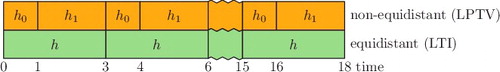
The non-equidistant sampling sequence is shown in Figure 5. It has periodicity τ = 2 with h ₀ = 1 and h ₁ = 2.

Figure 5. Time line of the non-equidistant sampling sequence. Control for the equidistant sampling sequence with period h = h ₀ + h ₁ is conservative since not all control points are exploited. To improve performance, control for the non-equidistant sampling sequence h ₀, h ₁ is pursued.

7.2 System

Consider the continuous-time system of Example 2 in Åström, Hagander, and Sternby (1984): (26) $$\begin{array}{c}\hfill H^c=\frac{1}{{(s+1)}^3}\stackrel{s}{=}\left[\begin{array}{cc}{A}^c& B^c\\ C^c& D^c\end{array}\right]=\left[\begin{array}{cccc}0& 1& 0& 0\\ 0& 0& 1& 0\\ -1& -3& -3& 1\\ 1& 0& 0& 0\end{array}\right],\end{array}$$(26) with zero-order-hold discretisation (27) $$\begin{array}{c}\hfill H\stackrel{s}{=}\left[\begin{array}{cc}{A}_k^H& B_k^H\\ C^H& D^H\end{array}\right]=\left[\begin{array}{cc}{e}^{A^c{h}_k}& {\left(A^c\right)}^{-1}(A_k^H-I)B^c\\ C^c& D^c\end{array}\right],\end{array}$$(27) where h _k is the sampling interval. Since D ^H  = 0, H is not directly invertible and the procedure in Remark 2.1 is followed. As a consequence, the inverse system F is non-reversible (see also Section 4.4).

As shown in Åström et al. (1984), for 0 < h _k < 1.8399, there is one minimum-phase and one nonminimum-phase zero, and for h _k ≥ 1.8399, both zeros are minimum phase. For the non-equidistant sampling sequence in Figure 5, one of the poles of LPTV system F alternates between stable and unstable.

It follows directly from Figure 5 that the smallest equidistant sampling sequence has period h = h ₀ + h ₁ = 3. The corresponding LTI system is thus minimum phase.

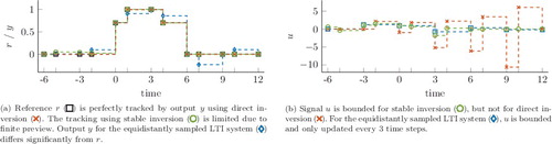
The reference trajectory r is shown in Figure 6(a).

Figure 6. Stable inversion generates bounded u, whereas direct inversion generates unbounded u. The performance of stable inversion is limited due to finite preview. The performance of the equidistant sampled LTI system is low due to an inexact inverse.

7.3 Application in feedforward control

In this section, an application in inverse model feedforward control is considered. True system H is assumed to be exactly known and F = H ⁻¹, with H in (27(27) $$\begin{array}{c}\hfill H\stackrel{s}{=}\left[\begin{array}{cc}{A}_k^H& B_k^H\\ C^H& D^H\end{array}\right]=\left[\begin{array}{cc}{e}^{A^c{h}_k}& {\left(A^c\right)}^{-1}(A_k^H-I)B^c\\ C^c& D^c\end{array}\right],\end{array}$$(27) ).

Regular inversion of the minimum-phase LTI system with period h = 3 yields input u shown in Figure 6(b). Note that u is only updated after 3 time units, and constant in-between. Applying this input to the true LPTV system H yields the output in Figure 6(a). Due to the mismatch between the LTI system used for inversion and the true LPTV system, the output y differs from the reference r. The results show the importance of LPTV inversion techniques.

The results in Figure 6 show that direct inversion of LPTV system H through (2(2) $$\begin{array}{c}\hfill F\stackrel{s}{=}\left[\begin{array}{cc}{A}_k& B_k\\ C_k& D_k\end{array}\right]=\left[\begin{array}{cc}{A}_k^H-B_k^H{\left(D_k^H\right)}^{-1}{C}_k^H& B_k^H{\left(D_k^H\right)}^{-1}\\ -{\left(D_k^H\right)}^{-1}{C}_k^H& {\left(D_k^H\right)}^{-1}\end{array}\right].\end{array}$$(2) ) yields perfect tracking y = r. However, input u is unbounded since F is unstable.

To obtain a bounded u and exact tracking, the stable inversion approach for LPTV systems as outlined in Figure 4 is used. Since F is non-reversible, Corollary 4.1 and Theorem 5.1 are used. The monodromy matrix Ψ in (10(10) $$\begin{array}{c}\hfill \Psi =A_{\tau -1}{A}_{\tau -2}\cdots A_0.\end{array}$$(10) ) has two eigenvalues inside and one outside the unit circle. A static transformation T _k  = T ₀ consisting of eigenvectors of Ψ is used (see Corollary 4.1). The stable inversion solution is obtained through Theorem 5.1. Figure 6(b) shows that stable inversion generates bounded u as desired.

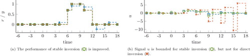
The tracking in Figure 6(a) is non-exact due to finite-time effects (Middleton, Chen, & Freudenberg, 2004). To improve performance, the interval length is increased by starting at time −6, with r initially zero. The addition of this preview time results in a performance improvement for stable inversion as desired (see Figure 7). The addition of even more preview time further improves the performance.

Figure 7. Additional preview improves the performance of stable inversion compared to Figure 6.

7.4 Application in iterative learning control

In this section, an application in iterative learning control (ILC) is considered. In ILC, the same task is repeated and deterministic uncertainties are compensated by learning from past data using a system model; see also Bristow, Tharayil, and Alleyne (2006).

The ILC update law is based on the closed-loop model $\widehat{H}=0.8H$, with H in (27(27) $$\begin{array}{c}\hfill H\stackrel{s}{=}\left[\begin{array}{cc}{A}_k^H& B_k^H\\ C^H& D^H\end{array}\right]=\left[\begin{array}{cc}{e}^{A^c{h}_k}& {\left(A^c\right)}^{-1}(A_k^H-I)B^c\\ C^c& D^c\end{array}\right],\end{array}$$(27) ). The error dynamics are given by (28) $$\begin{array}{c}\hfill e^{(j+1)}=e^{\left(j\right)}-H(u^{(j+1)}-u^{\left(j\right)}),e^{\left(0\right)}=r,\end{array}$$(28) with trial number j = 0, 1, …, and input u. The learning update is given by (29) $$\begin{array}{c}\hfill u^{(j+1)}=u^{\left(j\right)}+\alpha F{e}^{\left(j\right)},u^{\left(0\right)}=0,\end{array}$$(29) with learning filter $F={\widehat{H}}^{-1}$ and learning factor α = 0.5. Note that if αF = H ⁻¹, error e ^{(j + 1)} is zero as desired.

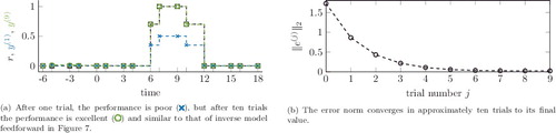
The results for the reference signal r in Figure 7(a) are shown in Figure 8. Since α ≠ 1, it takes several trials for the algorithm to converge, as can be observed in the two-norm of the error shown in Figure 8(b). After approximately ten trials, the update is converged to the same solution as with exact model inverse feedforward shown in Figure 7.

Figure 8. Application of stable inversion in ILC enables high-performance tracking with a nonexact model.

7.5 Summary

The case illustrates the use of stable inversion for non-equidistantly sampled systems, both in inverse model feedforward and ILC design. First of all, the case shows the advantage of LPTV control over LTI control for a non-equidistantly sampled system. Second, the case shows that direct inversion yields unbounded u whereas stable inversion generates bounded u. Third, the case shows that additional preview improves the performance of stable inversion. Indeed, stable inversion is exact for k _s → −∞. Finally, the application of LPTV stable inversion in ILC is demonstrated.

8. Case 3: position-dependent system

One of the challenges in motion systems is position-dependent behaviour, as present in, for example, wafer stages.

8.1 Wafer stage system

Wafer stages are key motion systems in wafer scanners used for the production of integrated circuits. A simplified 2D model of a wafer stage in the horizontal plane is considered as shown in Figure 9. The stage is actuated by force input u, can translate in x and y direction, and rotate in φ direction. The output is the distance $\widehat{x}$ between the metrology frame and the wafer stage, measured through an interferometer located on the metrology frame. The parameters are listed in Table 1.

Figure 9. Top view of wafer stage. The interferometer is fixed on the metrology frame and measures distance $\widehat{x}$ to the wafer stage which has degrees of freedom x, y, φ. If φ ≠ 0, position y effects measurement $\widehat{x}$.

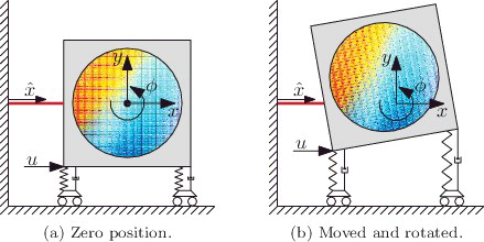
Table 1. Parameter values of the wafer stage system.

Parameter	Symbol	Value	Unit
Mass	m	50	kg
Inertia	I	2.08	kg m^2
Spring constant	c	10^6	N/m
Damping constant	d	2500	N s/m
Length	l	0.5	m

A typical wafer stage movement is a so-called meander pattern as illustrated in Figure 1(c); see also van der Meulen, Tousain, and Bosgra (2008). The position y is assumed to be prescribed by the periodic movement in Figure 11(a) and is controlled by a PD controller represented by the spring and damper in Figure 9. The desired trajectory ${\widehat{x}}^d$ for $\widehat{x}$ is also shown in Figure 11(a). The combination of y and ${\widehat{x}}^d$ generates the meander pattern shown in Figure 10. A key observation is that the $\widehat{x}$-dynamics are position dependent due to the influence of position y when φ ≠ 0.

Figure 10. Part of meander pattern constructed by ${\widehat{x}}^d,y$ in Figure 11(a).

The continuous-time state-space realisation (A ^c , B ^c , C ^c , D ^c ) of the $\widehat{x}$-dynamics, linearised around $\varphi ,\dot{\varphi }=0$, with input u, state ${\left(\begin{array}{cccc}x& \dot{x}& \varphi & \dot{\varphi }\end{array}\right)}^{\top }$, and output $\widehat{x}$ is (30) $$\begin{array}{c}\hfill \left[\begin{array}{cc}{A}^c& B^c\\ C_k^c& D^c\end{array}\right]=\left[\begin{array}{ccccc}0& 1& 0& 0& 0\\ 0& 0& 0& 0& \frac{1}{m}\\ 0& 0& 0& 1& 0\\ 0& 0& -\frac{1}{2}\frac{c{l}^2}{I}& -\frac{1}{2}\frac{d{l}^2}{I}& \frac{1}{2}\frac{l}{I}\\ 1& 0& y_k& 0& 0\end{array}\right].\end{array}$$(30) System H in (1) is the zero-order-hold discretised version of (30): (31) $$\begin{array}{c}\hfill H\stackrel{s}{=}\left[\begin{array}{cc}{A}^H& B^H\\ C_k^H& D^H\end{array}\right]=\left[\begin{array}{cc}{e}^{A^{c}h}& {\left(A^c\right)}^{-1}(A-I)B^c\\ C_k^c& D^c\end{array}\right],\end{array}$$(31) with sampling interval h = 0.001 s. Note that H is indeed position-dependent through C^H _k . Moreover, for the given parameters, the system is minimum phase if y _k ≥ 0, and nonminimum phase for y _k < 0. Since y _k is periodic, H is LPTV. Also note that H is strictly proper since D ^H  = 0, and thus F being the inverse of time-shifted H is non-reversible. Finally, note that the time-variance of C^H _k in H also introduces time-variance in A _k of F (see (2(2) $$\begin{array}{c}\hfill F\stackrel{s}{=}\left[\begin{array}{cc}{A}_k& B_k\\ C_k& D_k\end{array}\right]=\left[\begin{array}{cc}{A}_k^H-B_k^H{\left(D_k^H\right)}^{-1}{C}_k^H& B_k^H{\left(D_k^H\right)}^{-1}\\ -{\left(D_k^H\right)}^{-1}{C}_k^H& {\left(D_k^H\right)}^{-1}\end{array}\right].\end{array}$$(2) )).

8.2 Nonminimum-phase system

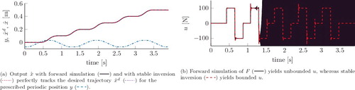
Forward time simulation of F with reference $r={\widehat{x}}^d$ and trajectory y in Figure 11(a) yields the unbounded signal u shown in Figure 11(b). Since F is non-reversible, it follows from Figure 4 that Theorem 5.1 with static transformation T _k  = T ₀ in Corollary 4.1 yields the stable inversion solution with bounded u. The monodromy matrix Ψ reveals one unstable and three stable states. The resulting signal u is shown in Figure 11(b) and is indeed bounded. The output position $\widehat{x}$ perfectly tracks the desired trajectory ${\widehat{x}}^d$ as shown in Figure 11(a).

Figure 11. Prescribed position y introduces position-dependence resulting in an LPTV system that is unstable. With stable inversion, a bounded solution u resulting in perfect tracking is obtained.

8.3 Minimum-phase system

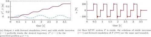
Consider the trajectory y in Figure 12(a). For this trajectory, the monodromy matrix Ψ indicates F is stable. Indeed, y _k < 0 for some k, but this does not necessarily lead to unstable F. Since F is stable, the stable inversion solution reduces to forward simulation of F (see Corollary 5.2). The results are shown in Figure 12(b) and show exact tracking.

Figure 12. Prescribed position y introduces position-dependence resulting in an LPTV system that is stable. The stable inversion solution reduces to that of forward simulation and yields perfect tracking.

8.4 Summary

The results show that if the LPTV system F is unstable, a bounded solution u is found, whereas if F is stable, the direct inversion result is recovered. The case demonstrates the application of the proposed LPTV stable inversion approach to position-dependent systems with periodic tasks.

9. Conclusion

In practice, many systems are LTV, yet exhibit periodicity, rendering them LPTV. Examples include, position-dependent systems with periodic tasks, multirate systems, and non-equidistantly sampled systems. System inversion is essential for tracking control applications, including feedforward and learning control. Perfect tracking of reference trajectories can be obtained via stable inversion. The stable inversion approach is based on a dichotomy of the system into a stable and unstable part. Such a dichotomy always exists for LTI systems (under mild conditions). In this paper, it is shown that such a dichotomy may not exist for general LTV systems, hampering the use of stable inversion.

By exploiting the periodicity, a dichotomy for LPTV systems is established. In fact, there always exists a dichotomy for LPTV systems, under similar mild conditions as for LTI systems. In this paper, this dichotomy is exploited to develop a stable inversion approach for LPTV systems, enabling perfect tracking of general reference trajectories. The approach is demonstrated for reversible systems, in feedforward and learning control, and for position-dependent systems. For reversible systems, the stable inversion approach simplifies considerably. An overview of the complete approach can be found in Figure 4.

The presented stable inversion for LPTV systems enables feedforward and learning control design for an important class of systems.

The performance of stable inversion strongly depends on the amount of preview, as also observed in Section 7. Future research related to this focuses on the role of preview and in particular on deriving bounds similar as for the LTI case (Middleton et al., 2004). From a broader perspective, future research focuses on exploiting the structure associated with LPTV systems in general feedforward and ILC techniques, and their connection to zeros of such systems (e.g. Zamani, Bottegal, & Anderson, 2016). Finally, the developed approach will be experimentally implemented, e.g. related to the work in van Zundert, Oomen, et al. (2016).

Disclosure statement

No potential conflict of interest was reported by the authors.

Additional information

Funding

This work is part of the research programme Robust Cyber-Physical Systems (RCPS) [number 12694] and Innovational Research Incentives Scheme under the VENI grant ‘Precision Motion: Beyond the Nanometer’ [number 13073]; both are (partly) financed by the Netherlands Organisation for Scientific Research (NWO).

Appendices

Appendix 1 Proof of Theorem 4.1

Proof:

If Ψ has no eigenvalues on the unit circle, so does $\tilde{\Psi }$ and an exponential dichotomy exists. Let (11(11) $$\begin{array}{c}\hfill \tilde{\Psi }={\tilde{A}}_{\tau -1}{\tilde{A}}_{\tau -2}\cdots {\tilde{A}}_0=\left(\begin{array}{cc}{\tilde{\Psi }}^s& 0\\ 0& {\tilde{\Psi }}^u\end{array}\right),\end{array}$$(11) ) be satisfied, then the autonomous system (A1) $$\begin{array}{c}\hfill {\tilde{x}}_{k+1}=\tilde{\Psi }{\tilde{x}}_k\end{array}$$(A1) has fundamental matrix solution (A2) $$\begin{array}{c}\hfill {\tilde{X}}_k={\left(\tilde{\Psi }\right)}^k=\left(\begin{array}{cc}{\left({\tilde{\Psi }}^s\right)}^k& 0\\ 0& {\left({\tilde{\Psi }}^u\right)}^k\end{array}\right).\end{array}$$(A2) Since $|{\lambda }_i\left({\tilde{\Psi }}^s\right)|<1$, ∀i, there exist constants K ^s > 0 and 0 < p ^s < 1 such that (A3) $$\begin{array}{c}\hfill \parallel {\left({\tilde{\Psi }}^s\right)}^k\parallel \le K^s{\left(p^s\right)}^k.\end{array}$$(A3) Similarly, since $|{\lambda }_i\left({\tilde{\Psi }}^u\right)|>1$, ∀i, there exist constants K ^u > 0 and 0 < p ^u < 1 such that (A4) $$\begin{array}{c}\hfill \parallel {\left({\tilde{\Psi }}^u\right)}^k\parallel \le K^u{\left({\left(p^u\right)}^{-1}\right)}^k.\end{array}$$(A4) Consequently, for (A5) $$\begin{array}{c}\hfill P=\left(\begin{array}{cc}{I}_s& 0\\ 0& 0\end{array}\right),\end{array}$$(A5) with I _s the identity matrix of size ${\tilde{\Psi }}^s$, it follows (A6) $$\begin{array}{cccc}\hfill ∥X_{n}P{X}_m^{-1}∥& \le K^s{\left(p^s\right)}^{n-m},\hfill & & n\ge m,\hfill \end{array}$$(A6) (A7) $$\begin{array}{cccc}\hfill ∥X_n(I-P)X_m^{-1}∥& \le K^u{\left(p^u\right)}^{m-n},\hfill & & m\ge n.\hfill \end{array}$$(A7) Hence, system (A1(A1) $$\begin{array}{c}\hfill {\tilde{x}}_{k+1}=\tilde{\Psi }{\tilde{x}}_k\end{array}$$(A1) ) with $\tilde{\Psi }$ in (11(11) $$\begin{array}{c}\hfill \tilde{\Psi }={\tilde{A}}_{\tau -1}{\tilde{A}}_{\tau -2}\cdots {\tilde{A}}_0=\left(\begin{array}{cc}{\tilde{\Psi }}^s& 0\\ 0& {\tilde{\Psi }}^u\end{array}\right),\end{array}$$(11) ) satisfies an exponential dichotomy according to Definition 2.1 for K = max {K ^s , K ^u }, p = max {p ^s , p ^u }, and P in (A5(A5) $$\begin{array}{c}\hfill P=\left(\begin{array}{cc}{I}_s& 0\\ 0& 0\end{array}\right),\end{array}$$(A5) ).

Appendix 2 Proof of Theorem 4.2

Proof:

The transformed system $\tilde{F}$ has monodromy matrix $\tilde{\Psi }={\tilde{A}}_{\tau -1}{\tilde{A}}_{\tau -2}\cdots {\tilde{A}}_0=T_{\tau }^{-1}\Psi T_0$. For τ-periodic T _k , it holds T _τ = T ₀ and hence $\tilde{\Psi }=T_0^{-1}\Psi T_0$. By selecting T ₀ as generalised eigenvectors of Ψ, condition (11(11) $$\begin{array}{c}\hfill \tilde{\Psi }={\tilde{A}}_{\tau -1}{\tilde{A}}_{\tau -2}\cdots {\tilde{A}}_0=\left(\begin{array}{cc}{\tilde{\Psi }}^s& 0\\ 0& {\tilde{\Psi }}^u\end{array}\right),\end{array}$$(11) ) can be satisfied by proper ordering of the eigenvectors. It then directly follows from Theorem 4.1 that $\tilde{F}$ satisfies an exponential dichotomy according to Definition 2.1.

Appendix 3 Proof of Lemma 4.2

For transformation T _k in (12(12) $$\begin{array}{cc}\hfill T_k& =A_{k-1}{T}_{k-1}{\widehat{A}}^{-1},k\in [1,\tau -1],\hfill \end{array}$$(12) ), it follows using (6(6) $$\tilde{F}\stackrel{s}{=}\left[\begin{array}{cc}{\tilde{A}}_k& {\tilde{B}}_k\\ {\tilde{C}}_k& {\tilde{D}}_k\end{array}\right]=\left[\begin{array}{cc}{T}_{k+1}^{-1}{A}_k{T}_k& T_{k+1}^{-1}{B}_k\\ C_k{T}_k& D_k\end{array}\right].$$(6) ) that (C1) $${\tilde{A}}_k=T_{k+1}^{-1}{A}_k{T}_k$$(C1) (C2) $$={\left(A_k{T}_k{\widehat{A}}^{-1}\right)}^{-1}{A}_k{T}_k$$(C2) (C3) $$=\widehat{A}{\left(A_k{T}_k\right)}^{-1}\left(A_k{T}_k\right)$$(C3) (C4) $$=\widehat{A}$$(C4) for all k. Periodicity of T _k can be shown by successive substitution: (C5) $$T_{\tau }=(A_{\tau -1}{A}_{\tau -2}\cdots A_0)T_0{\widehat{A}}^{-\tau }$$(C5) (C6) $$=\Psi T_0{\left({\left(T_0^{-1}\Psi T_0\right)}^{\frac{1}{\tau }}\right)}^{-\tau }$$(C6) (C7) $$=\Psi T_0{\left(T_0^{-1}\Psi T_0\right)}^{-1}$$(C7) (C8) $$=\Psi T_0{T}_0^{-1}{\Psi }^{-1}{T}_0$$(C8) (C9) $$=T_0.$$(C9) Combining this result with (12(12) $$\begin{array}{cc}\hfill T_k& =A_{k-1}{T}_{k-1}{\widehat{A}}^{-1},k\in [1,\tau -1],\hfill \end{array}$$(12) ) shows that T _k is periodic with period τ. Note that ${\widehat{A}}^{-1}$ should exist which is directly satisfied if T ₀ and Ψ are invertible. Indeed, the reversibility condition ensures A _k , ∀k and thereby Ψ in (10(10) $$\begin{array}{c}\hfill \Psi =A_{\tau -1}{A}_{\tau -2}\cdots A_0.\end{array}$$(10) ) are invertible.

Appendix 4 Proof of Theorem 4.3

Proof:

Lemma 4.2 yields ${\tilde{A}}_k=\widehat{A}$, ∀k such that by (11(11) $$\begin{array}{c}\hfill \tilde{\Psi }={\tilde{A}}_{\tau -1}{\tilde{A}}_{\tau -2}\cdots {\tilde{A}}_0=\left(\begin{array}{cc}{\tilde{\Psi }}^s& 0\\ 0& {\tilde{\Psi }}^u\end{array}\right),\end{array}$$(11) ) it follows that $\tilde{\Psi }={\left(\widehat{A}\right)}^{\tau }=T_0^{-1}\Psi T_0$, for $\widehat{A}$ in (13(13) $$\begin{array}{c}\hfill \widehat{A}={\left(T_0^{-1}\Psi T_0\right)}^{\frac{1}{\tau }},\end{array}$$(13) ). With T ₀ given by Theorem 4.2, $\tilde{F}$ satisfies an exponential dichotomy. Moreover, condition (11(11) $$\begin{array}{c}\hfill \tilde{\Psi }={\tilde{A}}_{\tau -1}{\tilde{A}}_{\tau -2}\cdots {\tilde{A}}_0=\left(\begin{array}{cc}{\tilde{\Psi }}^s& 0\\ 0& {\tilde{\Psi }}^u\end{array}\right),\end{array}$$(11) ) is satisfied and hence (D1) $$\begin{array}{cc}\hfill \widehat{A}& ={\left(\tilde{\Psi }\right)}^{\frac{1}{\tau }}=\left(\begin{array}{cc}{\left({\tilde{\Psi }}^s\right)}^{\frac{1}{\tau }}& 0\\ 0& {\left({\tilde{\Psi }}^u\right)}^{\frac{1}{\tau }}\end{array}\right),\hfill \end{array}$$(D1) which shows that the unstable and stable parts are separated.

Appendix 5 Proof of Theorem 5.1

Proof:

From (15a(15a) $$x_{k+1}^s=A_k^{ss}{x}_k^s+A_k^{su}{x}_k^u+B_k^s{r}_k,$$(15a) ) and (15b(15b) $$x_{k+1}^u=A_k^{us}{x}_k^s+A_k^{uu}{x}_k^u+B_k^u{r}_k,$$(15b) ) follows that there is an affine relation between x ^s and x ^u . Let this relation be given by (17b(17b) $$x_k^u=S_k{x}_k^s+g_k,$$(17b) ) for some S _k , g _k . Substituting (17b(17b) $$x_k^u=S_k{x}_k^s+g_k,$$(17b) ) in (15a(15a) $$x_{k+1}^s=A_k^{ss}{x}_k^s+A_k^{su}{x}_k^u+B_k^s{r}_k,$$(15a) ) yields (17a(17a) $$x_{k+1}^s=\left(A_k^{ss}+A_k^{su}{S}_k\right)x_k^s+B_k^s{r}_k+A_k^{su}{g}_k,$$(17a) ) which can be solved forward in time with $x_{k_s}^s=0$. Eliminating x ^u from (15b(15b) $$x_{k+1}^u=A_k^{us}{x}_k^s+A_k^{uu}{x}_k^u+B_k^u{r}_k,$$(15b) ) using (17b(17b) $$x_k^u=S_k{x}_k^s+g_k,$$(17b) ), substituting (17a(17a) $$x_{k+1}^s=\left(A_k^{ss}+A_k^{su}{S}_k\right)x_k^s+B_k^s{r}_k+A_k^{su}{g}_k,$$(17a) ), and rearranging terms yields (E1a) $$\begin{array}{c}\hfill S_{k+1}{x}_{k+1}^s+g_{k+1}=A_k^{us}{x}_k^s+A_k^{uu}(S_k{x}_k^s+g_k)+B_k^u{r}_k,\end{array}$$(E1a) (E1b) $$\begin{array}{ccc}& & S_{k+1}((A_k^{ss}+A_k^{su}{S}_k)x_k^s+B_k^s{r}_k+A_k^{su}{g}_k)+g_{k+1}\hfill \\ & & =A_k^{us}{x}_k^s+A_k^{uu}(S_k{x}_k^s+g_k)+B_k^u{r}_k,\hfill \end{array}$$(E1b) (E1c) $$\begin{array}{ccc}& & (S_{k+1}{A}_k^{ss}+S_{k+1}{A}_k^{su}{S}_k-A_k^{us}-A_k^{uu}{S}_k)x_k^s\hfill \\ & & =-S_{k+1}{B}_k^s{r}_k-S_{k+1}{A}_k^{su}{g}_k-g_{k+1}+A_k^{uu}{g}_k+B_k^u{r}_k,\hfill \end{array}$$(E1c) which is of the form ${\mathcal{A}}_k{x}_k^s={\mathcal{B}}_k$. Since it holds for all x^s _k , it follows that ${\mathcal{A}}_k=0$ which yields (17c(17c) $$S_k={\left(A_k^{uu}-S_{k+1}{A}_k^{su}\right)}^{-1}\left(S_{k+1}{A}_k^{ss}-A_k^{us}\right),$$(17c) ), and ${\mathcal{B}}_k=0$ which yields (17d(17d) $$g_k={\left(S_{k+1}{A}_k^{su}-A_k^{uu}\right)}^{-1}\left(B_k^u{r}_k-S_{k+1}{B}_k^s{r}_k-g_{k+1}\right),$$(17d) ). Next, (17c(17c) $$S_k={\left(A_k^{uu}-S_{k+1}{A}_k^{su}\right)}^{-1}\left(S_{k+1}{A}_k^{ss}-A_k^{us}\right),$$(17c) ) and (17d(17d) $$g_k={\left(S_{k+1}{A}_k^{su}-A_k^{uu}\right)}^{-1}\left(B_k^u{r}_k-S_{k+1}{B}_k^s{r}_k-g_{k+1}\right),$$(17d) ) are solved backward in time for some $S_{k_e}$ and $g_{k_e}$, respectively. Here, $S_{k_e}=0$ and $g_{k_e}=0$ are selected.

References

- Åström, K. , Hagander, P. , & Sternby, J. (1984). Zeros of sampled systems. Automatica , 20 (1), 31–38.
- Bayard, D. S. (1994). Extended horizon liftings for stable inversion of nonminimum-phase systems. Transactions on Automatic Control , 39 (6), 1333–1338.
- Berger, T. , Ilchmann, A. , & Wirth, F. (2015). Zero dynamics and stabilization for analytic linear systems. Acta Applicandae Mathematicae , 138 (1), 17–57.
- Bittanti, S. , & Colaneri, P . (2009). Periodic systems - filtering and control . London: Springer-Verlag.
- Boeren, F. , Oomen, T. , & Steinbuch, M. (2015). Iterative motion feedforward tuning: A data-driven approach based on instrumental variable identification. Control Engineering Practice , 37 , 11–19.
- Bolder, J. , & Oomen, T. (2015). Rational basis functions in iterative learning control - with experimental verification on a motion system. Transactions on Control Systems Technology , 23 (2), 722–729.
- Bristow, D. , Tharayil, M. , & Alleyne, A. (2006). A survey of iterative learning control. Control Systems Magazine , 26 (3), 96–114.
- Butterworth, J. A. , Pao, L. Y. , & Abramovitch, D. Y. (2008). The effect of nonminimum-phase zero locations on the performance of feedforward model-inverse control techniques in discrete-time systems. In Proceedings of the 2008 American control conference , Seattle, Washington (pp. 2696–2702). IEEE.
- Chen, D. (1993). An iterative solution to stable inversion of nonminimum phase systems. In Proceedings of the 1993 American control conference , San Francisco, CA (pp. 2960–2964). IEEE.
- Chen, T. , & Francis, B. A . (1995). Optimal sampled-data control systems . London: Springer.
- Clayton, G. M. , Tien, S. , Leang, K. K. , Zou, Q. , & Devasia, S. (2009). A review of feedforward control approaches in nanopositioning for high-speed SPM. Journal of Dynamic Systems, Measurement, and Control , 131 (6), 061101–061101–19.
- Coppel, W. (1978). Dichotomies in stability theory. In Lecture notes in mathematics (Vol. 629). Berlin-Heidelberg: Springer-Verlag.
- Devasia, S. (1997). Output tracking with nonhyperbolic and near nonhyperbolic internal dynamics: Helicopter hover control. In Proceedings of the 1997 American control conference , Albuquerque, NM (Vol. 3, pp. 1439–1446).
- Devasia, S. , Chen, D. , & Paden, B. (1996). Nonlinear inversion-based output tracking. Transactions on Automatic Control , 41 (7), 930–942.
- Devasia, S. , & Paden, B. (1994). Exact output tracking for nonlinear time-varying systems. In Proceedings of 33rd conference on decision and control , Lake Buena Vista, FL (pp. 2346–2355). IEEE.
- Devasia, S. , & Paden, B. (1998). Stable inversion for nonlinear nonminimum-phase time-varying systems. Transactions on Automatic Control , 43 (2), 283–288.
- Fujimoto, H. , & Hori, Y. (2002). High-performance servo systems based on multirate sampling control. Control Engineering Practice , 10 (7), 773–781.
- Halanay, A. , & Ionescu, V. (1994). Time-varying discrete linear systems: Input–output operators. Riccati equations. Disturbance attenuation (Vol. 68). Birkhäuser Verlag.
- Hill, A. T. , & Ilchmann, A. (2011). Exponential stability of time-varying linear systems. IMA Journal of Numerical Analysis , 31 (3), 865–885.
- Hirschorn, R. M. (1979). Invertibility of multivariable nonlinear control systems. Transactions on Automatic Control , 24 (6), 855–865.
- Hunt, L. , Meyer, G. , & Su, R. (1996). Noncausal inverses for linear systems. Transactions on Automatic Control , 41 (4), 608–611.
- Jetto, L. , Orsini, V. , & Romagnoli, R. (2015). A mixed numerical-analytical stable pseudo-inversion method aimed at attaining an almost exact tracking. International Journal of Robust and Nonlinear Control , 25 (6), 809–823.
- Marro, G. , Prattichizzo, D. , & Zattoni, E. (2002). Convolution profiles for right inversion of multivariable non-minimum phase discrete-time systems. Automatica , 38 (10), 1695–1703.
- van der Meulen, S. H. , Tousain, R. L. , & Bosgra, O. H. (2008). Fixed structure feedforward controller design exploiting iterative trials: Application to a wafer stage and a desktop printer. Journal of Dynamic Systems, Measurement, and Control , 130 (5), 051006:1–16.
- Middleton, R. , Chen, J. , & Freudenberg, J. (2004). Tracking sensitivity and achievable H ∞ performance in preview control. Automatica , 40 (8), 1297–1306.
- Moylan, P. (1977). Stable inversion of linear systems. Transactions on Automatic Control , 22 (1), 74–78.
- Ohnishi, W. , & Fujimoto, H. (2016). Tracking control method for a plant with continuous time unstable zeros: Finite preactuation based on state trajectory regeneration by using redundant order polynomial. In 55th Conference on decision and control , Las Vegas, NE (pp. 4015–4020). IEEE.
- Papaschinopoulos, G. (1986). Exponential separation, exponential dichotomy, and almost periodicity of linear difference equations. Journal of Mathematical Analysis and Applications , 120 (1), 276–287.
- Pavlov, A. , & Pettersen, K. Y. (2008). A new perspective on stable inversion of non-minimum phase nonlinear systems. Modeling, Identification and Control , 29 (1), 29–35.
- Silverman, L. M. (1969). Inversion of multivariable linear systems. Transactions on Automatic Control , 14 (3), 270–276.
- Sogo, T. (2010). On the equivalence between stable inversion for nonminimum phase systems and reciprocal transfer functions defined by the two-sided Laplace transform. Automatica , 46 (1), 122–126.
- Zamani, M. , Bottegal, G. , & Anderson, B. D. (2016). On the zero-freeness of tall multirate linear systems. Transactions on Automatic Control , 61 (11), 3611.
- Zattoni, E. (2014). Geometric methods for invariant-zero cancellation in linear multivariable systems with application to signal rejection with preview. Asian Journal of Control , 16 (5), 1289–1299.
- Zou, Q. (2009). Optimal preview-based stable-inversion for output tracking of nonminimum-phase linear systems. Automatica , 45 (1), 230–237.
- Zou, Q. , & Devasia, S. (1999). Preview-based stable-inversion for output tracking of linear systems. Journal of Dynamic Systems, Measurement, and Control , 121 (4), 625–630.
- Zou, Q. , & Devasia, S. (2004). Preview-based optimal inversion for output tracking: Application to scanning tunneling microscopy. Transactions on Control Systems Technology , 12 (3), 375–386.
- Zou, Q. , & Devasia, S. (2007). Precision preview-based stable-inversion for nonlinear nonminimum-phase systems: The VTOL example. Automatica , 43 (1), 117–127.
- van Zundert, J. , Bolder, J. , Koekebakker, S. , & Oomen, T. (2016). Resource-efficient ILC for LTI/LTV systems through LQ tracking and stable inversion: Enabling large feedforward tasks on a position-dependent printer. Mechatronics , 38 , 76–90.
- van Zundert, J. , & Oomen, T. (2017). An approach to stable inversion of LPTV systems with application to a position-dependent motion system. In Proceedings of the 2017 American control conference , Seattle, Washington (pp. 4890–4895). IEEE.
- van Zundert, J. , Oomen, T. , Goswami, D. , & Heemels, W. (2016). On the potential of lifted domain feedforward controllers with a periodic sampling sequence. In Proceedings of the 2016 American control conference , Boston, MA (pp. 4227–4232). IEEE.