Stability analysis and stabilisation in linear continuous-time periodic systems by complex scaling

ABSTRACT

By scaling in the complex domain (namely, complex scaling) the return difference relations of linear continuous-time periodic (LCP) feedback systems, we generalise the 2-regularised stability criteria for asymptotic stability in this paper. The stability conditions of the generalised criterion are necessary and sufficient, and involve neither contour and locus orientation specification, nor open-loop Floquet factorisation and its eigenvalues distribution. Finite-dimensional implementation of the suggested criteria is considered via a two-step truncation approach. The finite-dimensional criteria are implementable either graphically with locus plotting, or numerically without locus plotting, besides retaining the aforementioned technical advantages. Furthermore, also exploiting the complex scaling technique, stabilisation of LCP systems with static state feedback is worked out in the internal or external stability sense, whose alternative interpretations in terms of the small-gain theorem and the Gronwall inequality are explicated. To illustrate the main results, the lossy Mathieu differential equation is investigated.

KEYWORDS:

• Periodic
• stability
• stabilisation
• complex scaling
• finite-dimensional implementation

1. Introduction

Stability analysis and stabilisation are inevitably more difficult when linear continuous-time periodic (LCP) systems (Bittanti & Colaneri, 2001; Farkas, 1994; Halanay, 1966; Montagnier, Spiteri, & Angeles, 2004; Zhou & Hagiwara, 2005; Zhou, Hagiwara, & Araki, 2002) are considered, due to issues in transition matrix computing and Floquet factorisation for Floquet-Lyapunov coordinates transformation. We are frequently confronted with LCP models in engineering applications such as modelling flapping dynamics of helicopter rotor blades (Dugundji & Wendelll, 1983) and describing rolling motion of ships in waves (Allievi & Soudack, 1990). Miscellaneous stability terminologies and techniques for LCP systems are discussed. For example, absolute stability of LCP systems with nonlinearities subject to integral quadratic constraints is dealt with in Kao, Megretski, and J&quote;onsson (2001) and Yakubovich (1988) by the cutting plane algorithm and the Hamiltonian approach, respectively, while input/output stability and Youla-style parametrization of stabilising controllers are discussed in Cantoni and Glover (2000) via the graph representation. The Fredholm theory is adopted in stability testing and $H_2$ computation by Lampe and Rossenwasser (2010, 2011). As is well known, the Floquet theorem reflects asymptotic stability in LCP systems by eigenvalues distribution of the so-called monodromies that can only be calculated generally via numerical integral. Asymptotic stability in LCP systems has also been attacked by the Lyapunov method (Bolzern & Colaneri, 1988) and the harmonic analysis (Zhou et al., 2002). Perturbation methods to study stability in LCP systems can be found in Nayfeh and Mook (1979); Zhou and Qian (2017a). Indeed, LCP systems belong to a big class of complicated systems nearest to LTI ones, which have been investigated quite intensively via the harmonic analysis (Zhou & Hagiwara, 2005; Zhou et al., 2002; Zhou, Lu, & Qian, 2016).

In feedback configurations with LCP plants, a stability criterion is suggested in Hall and Wereley (1990), which is integral-operator-based (namely, integral operator modelling of periodic systems). Regarding infinite-dimensionality and truncation convergence issues in the Hill-determinant, the result validity in Hall and Wereley (1990) was not given. Recently, a generalised Nyquist criterion in 2-regularised determinant is reported in Zhou and Hagiwara (2005). Although implementation algorithms are also contrived in Zhou and Hagiwara (2005), the algorithms entail Floquet factorizations for providing open-loop poles distribution and guarantee numerical convergence in truncating infinite-dimensional Toeplitz operators during locus plotting. As is well known, transition matrices in LCP systems are hard to fix and so are their Floquet factorizations. Since irreducible/reducible Floquet factorizations may yield controllability/observability discrepancies (Zhou et al., 2016), internal stability may not be reflected appropriately and rigorously.

To surmount various algebraic and structural obstacles in stability analysis and stabilisation (Zhou, Qian, & Lu, 2017), the complex scaling technique is suggested and brings us with fruitful results in complicated feedback systems, say fractional-order (Zhou, 2017), sampled-data (Zhou & Qian, 2017b), time-delayed (Zhou, Gao, & Lu, 2018) and even nonlinear systems (Zhou, 2018). It must be stressed that although the same mathematical tool is adopted in the studies, different types of return difference relations with essentially different properties must be dealt with. This is also the case in LCP systems, whose complex-domain relations are infinite-dimensional.

In this paper, the feedback connections with LCP plants and controllers are attacked via complex scaling. More precisely, the harmonic return difference relation (Zhou & Hagiwara, 2005) is re-written into a complex scaling manner by separating the open- and closed-loop characteristic polynomials, with respect to prescribed scaling comparators. Based on the argument principle of complex analysis, we validate rigorously the complex scaling 2-regularised criteria for asymptotic stability in LCP systems (Zhou, 2013). The suggested stability conditions are necessary and sufficient. Different from the criteria of (Zhou & Hagiwara, 2005; Zhou et al., 2002), however, the complex scaling ones involve no open-loop Floquet factorisation and are stated with self-defined contour and locus orientation conditions. Implementation algorithms are proposed via truncating the harmonic transfer operators, in terms of finite-dimensional LTI system approximations. Moreover, the finite-dimensional criteria can be employed graphically with locus plotting, or numerically by computing complex argument incremental; the latter makes the approach be numerically tractable so that it is suitable for stabilisation as well.

Outline. Section 2 gives preliminaries to Toeplitz transformation of periodic functions and harmonic transfer operators. In Section 3, the complex scaling return difference relation is created, and the complex scaling stability criteria are claimed. Finite-dimensional implementation and its numerical convergence are considered in Section 4. Stabilization design for LCP systems is examined in Section 5. The lossy Mathieu equation is examined to illustrate the main results in Section 6. Conclusions are summarised in Section 7.

2. Notations and preliminaries to LCP systems

2.1. Notations and terminologies

In the paper, $|\cdot |$ denotes the absolute value of a scalar, the Euclidean vector norm and the induced matrix norm. $l_2$ is the set of all infinite-dimensional vectors $\underset{\_}{x}$ with $\sum _{-\mathrm{\infty }}^{+\mathrm{\infty }}|x_m{|}^2<\mathrm{\infty }$, where $x_m$ is the m-th entry of $\underset{\_}{x}$. $|\cdot {|}_{l_2/l_2}$ denotes the $l_2$-induced norm for an operator $(\cdot ):l_2\to l_2$. $L_2[0,h]$ is the linear space of all measurable functions $x\left(t\right)$ defined on $[0,h]$ with ${\int }_0^h|x\left(t\right){|}^{2}dt<\mathrm{\infty }$. $\mathbf{C}$ is the field of all complex numbers and $\mathbf{Z}$ is the ring of all integers. $\lambda (\cdot )$ denotes the set of all eigenvalues of $(\cdot )$, while the k-th one is meant by ${\lambda }_k(\cdot )$. We denote the subsets $L_{\mathrm{PCD}}[0,h]\subset L_2[0,h]$, $L_{\mathrm{PCC}}[0,h]\subset L_2[0,h]$, and $L_{\mathrm{AC}}[0,h]\subset L_2[0,h]$. PCD implies $f\left(t\right)\in L_{\mathrm{PCD}}[0,h]$ is piecewise continuous and differentiable a.e. (almost everywhere); PCC implies that $f\left(t\right)$ is piecewise continuous and its Fourier series is convergent a.e., and AC means that the Fourier series of $f\left(t\right)$ is absolutely convergent.

To understand the 2-regularised determinant, let ${\lambda }_i\left(A\right)$ denote the i-th eigenvalue of a linear compact operator $A:l_2\to l_2$ and $s_i\left(A\right):=\left({\lambda }_i\right(A^{\ast }A){)}^{1/2}$ be its i-th singular value. For p=1,2, the set of all compact operators satisfying $|A{|}_p:=\left(\sum _i{s}_i\right(A{)}^p{)}^{1/p}<\mathrm{\infty }$ is denoted by ${\mathbf{C}}_1$ and ${\mathbf{C}}_2$, respectively. The operators in ${\mathbf{C}}_1$ are trace class while those in ${\mathbf{C}}_2$ are Hilbert-Schmidt (Böttcher & Silbermann, 1990; Gohberg, Goldberg, & Krupnik, 2000). Clearly, ${\mathbf{C}}_1\subset {\mathbf{C}}_2$. For $A\in {\mathbf{C}}_1$, the operator trace and determinant $\mathrm{tr}\left(A\right):=\sum {\lambda }_i\left(A\right)$, $det(I+A)=\prod (1+{\lambda }_i(A\left)\right)$ are well-defined if the infinite summation and product converge. For $A\in {\mathbf{C}}_2$, let $R_2\left(A\right)=(I+A)\exp \{-A\}-I\in {\mathbf{C}}_1$. Thus, ${\det }_2(I+A):=det(I+R_2(A\left)\right)$ is the 2-regularised determinant of I+A.

Expand $X\left(t\right)\in L_2[0,h]$ to its Fourier series $\sum _{m=-\mathrm{\infty }}^{+\mathrm{\infty }}{X}_m{e}^{jm{\omega }_{h}t}$ with ${\omega }_h:=2\pi /h$. The Toeplitz transformation of $X\left(t\right)$, denoted by $\mathcal{T}\left\{X\right(t\left)\right\}$, maps $X\left(t\right)$ into a doubly infinite-dimensional block Toeplitz operator (or block Laurent operator (Gohberg, Goldberg, & Kaashoek, 1993, p. 564)) as $\mathcal{T}\left\{X\right(t\left)\right\}:=\left[\begin{array}{ccccc}\ddots & ⋮& ⋮& ⋮& \ddots \\ \cdots & X_0& X_{-1}& X_{-2}& \cdots \\ \cdots & X_1& X_0& X_{-1}& \cdots \\ \cdots & X_2& X_1& X_0& \cdots \\ \ddots & ⋮& ⋮& ⋮& \ddots \end{array}\right]=:\mathcal{X}$

2.2. Preliminaries to LCP systems

Firstly, consider the LCP system (1) $G:\{\begin{array}{l}\dot{x}=A\left(t\right)x+B\left(t\right)u\\ y=C\left(t\right)x\end{array}$(1) where $A\left(t\right),B\left(t\right)$ and $C\left(t\right)$ are h-periodically time-varying. Let $\mathrm{\Phi }(t,t_0)$ be the transition matrix. By the Floquet theorem (Lukes, 1982), if $A\left(t\right)\in L_2[0,h]$, then $\mathrm{\Phi }(t,0)$ is absolutely continuous in t and has Floquet factorisation $\mathrm{\Phi }(t,0)=P(t,0)e^{Qt}$, where $P(t,0)$ is absolutely continuous, nonsingular and h-periodic in t, and Q is a constant (probably complex) matrix. The system is asymptotically stable if and only if all eigenvalues of Q lie in the open left-half plane.

Secondly, we define $\mathcal{A}:=\mathcal{T}\left\{A\right(t\left)\right\}$, $\mathcal{B}:=\mathcal{T}\left\{B\right(t\left)\right\}$, $\mathcal{C}:=\mathcal{T}\left\{C\right(t\left)\right\}$, $\mathcal{P}:=\mathcal{T}\left\{P\right(t,0\left)\right\}$, $\mathcal{Q}:=\mathcal{T}\left\{Q\right\}=\mathrm{diag}[\cdots ,Q,Q,Q,\dots ]$ and $\mathcal{E}\left(s\right):=\mathrm{diag}[\cdots ,{\varphi }_{-1}(s)I,{\varphi }_0(s)I,{\varphi }_1(s)I,\dots ]$, where ${\varphi }_m\left(s\right):=s+jm{\omega }_h,m\in \mathbf{Z},s\in \mathbf{C}$ and I is the $n\times n$ identity matrix. In addition, $l_E:=\{\underset{\_}{x}\in l_2:\mathcal{E}(j0)\underset{\_}{x}\in l_2\}$, which is dense in $l_2$. It is easy to see that $\mathcal{P}\left(\mathcal{E}\right(j0)-\mathcal{Q}){\mathcal{P}}^{-1}$ and $\mathcal{E}\left(j0\right)-\mathcal{A}$ are unbounded and densely defined on $l_2$ and satisfy (2) $\mathcal{P}\left(\mathcal{E}\right(j0)-\mathcal{Q}){\mathcal{P}}^{-1}=\mathcal{E}\left(j0\right)-\mathcal{A}$(2) Moreover, the system is asymptotically stable if and only if all eigenvalues of $\mathcal{Q}-\mathcal{E}\left(j0\right)$ lie in the open left-half plane. Also, $\lambda (\mathcal{Q}-\mathcal{E}(j0\left)\right)=\left\{\lambda \right(Q)+jm{\omega }_h:m\in \mathbf{Z}\}=\lambda (\mathcal{A}-\mathcal{E}(j0\left)\right):=\mathrm{\Lambda }$.

Thirdly, we introduce the harmonic transfer operator of (1(1) $G:\{\begin{array}{l}\dot{x}=A\left(t\right)x+B\left(t\right)u\\ y=C\left(t\right)x\end{array}$(1) ) by (3) $\mathcal{G}\left(s\right):=\mathcal{C}\left(\mathcal{E}\right(s)-\mathcal{A}{)}^{-1}\mathcal{B}$(3) To ensure well-definedness of ${\mathcal{E}}^{-1}\left(s\right)$ and $\mathcal{G}\left(s\right)$, let us define a domain $\mathrm{\Omega }\subset \mathbf{C}$ to satisfy: (A1). Ω is simply connected and has a simple closed boundary $\tilde{\mathrm{\Omega }}$; also, $|\mathrm{Im}\left(s\right)|\le {\omega }_h$ over $s\in \mathrm{\Omega }$. (A2). For each $s\in \mathrm{\Omega }\setminus \mathrm{\Lambda }$, $\mathcal{E}\left(s\right)-\mathcal{Q}$ is an invertible mapping from $l_E$ to $l_2$. (A3). For each $s\in \mathrm{\Omega }$, $\mathcal{E}\left(s\right)$ is an invertible mapping from $l_E$ to $l_2$ with ${\mathcal{E}}^{-1}\left(s\right)$ being bounded.

When the domain Ω is meant as above, for all $s\in \mathrm{\Omega }\setminus \mathrm{\Lambda }$, we have (4) $\mathcal{P}\left(\mathcal{E}\right(s)-\mathcal{Q}{)}^{-1}{\mathcal{P}}^{-1}=(\mathcal{E}\left(s\right)-\mathcal{A}{)}^{-1}$(4) which says that $\mathcal{G}\left(s\right):l_2\to l_2$ is well-defined for all $s\in \mathrm{\Omega }\setminus \mathrm{\Lambda }$.

Finally, for each $s\in \mathrm{\Omega }$, it holds that (5) ${det}_2[\mathcal{I}-{\mathcal{E}}^{-1}(s\left)\mathcal{A}\right]=g\left(s\right){det}_2[\mathcal{I}-{\mathcal{E}}^{-1}(s\left)\mathcal{Q}\right]$(5) where $g\left(s\right)$ is analytic and vanishes nowhere over $s\in \mathrm{\Omega }$. Also, $\mathcal{I}-{\mathcal{E}}^{-1}\left(s\right)\mathcal{A}$ is invertible for each $s\in \mathrm{\Omega }\setminus \mathrm{\Lambda }$ and the inverse is bounded on $l_2$. In other words, asymptotic stability of (1(1) $G:\{\begin{array}{l}\dot{x}=A\left(t\right)x+B\left(t\right)u\\ y=C\left(t\right)x\end{array}$(1) ) is reflected by the zeros of ${det}_2[\mathcal{I}-{\mathcal{E}}^{-1}(s\left)\mathcal{A}\right]$. This is the starting point of the study.

3. Complex scaling stability criterion

In this section, we develop a complex scaling criterion for stability of LCP feedback connections. More precisely, let $A\left(t\right)$, $B\left(t\right)$, $C\left(t\right)\in L_{\mathrm{AC}}[0,h]\cap L_{\mathrm{PCD}}[0,h]$, to which an h-periodic output feedback $u=-K\left(t\right)y+v$ is installed. This yields us the closed-loop LCP system (6) $G_c:\{\begin{array}{l}\dot{x}=A_c\left(t\right)x+B\left(t\right)v\\ y=C\left(t\right)x\end{array}$(6) Here v is a new reference and assume that $K\left(t\right)\in L_{\mathrm{AC}}[0,h]\cap L_{\mathrm{PCD}}[0,h]$. Clearly, $A_c\left(t\right):=A\left(t\right)-B\left(t\right)K\left(t\right)C\left(t\right)\in L_{\mathrm{AC}}[0,h]\cap L_{\mathrm{PCD}}[0,h]$. $G_c$ can also be formed with a dynamic controller. Such cases bring no essential problems. For simplicity, we only address asymptotic stability of (6(6) $G_c:\{\begin{array}{l}\dot{x}=A_c\left(t\right)x+B\left(t\right)v\\ y=C\left(t\right)x\end{array}$(6) ) by examining stability conditions in term of the 2-regularised determinant.

3.1. Cauchy contour and 2-regularised determinant return difference relation

We recall by the block diagonal expression of $\mathcal{E}\left(j0\right)-\mathcal{Q}$ : (i) all eigenvalues of $\mathcal{E}\left(j0\right)-\mathcal{Q}$ are located in a vertical strip region; (ii) all the eigenvalues in the horizontal fundamental strip (7) ${\mathbf{C}}_f:=\{s\in \mathbf{C}:-{\omega }_h/2<\mathrm{Im}(s)\le {\omega }_h/2\}$(7) unfold themselves vertically to $-j\mathrm{\infty }$ and $j\mathrm{\infty }$ with period $j{\omega }_h$. Thus, if we know the eigenvalues distribution of $\mathcal{E}\left(j0\right)-\mathcal{Q}$ in ${\mathbf{C}}_f$, the whole eigenvalues distribution of $\mathcal{E}\left(j0\right)-\mathcal{Q}$ is clarified. 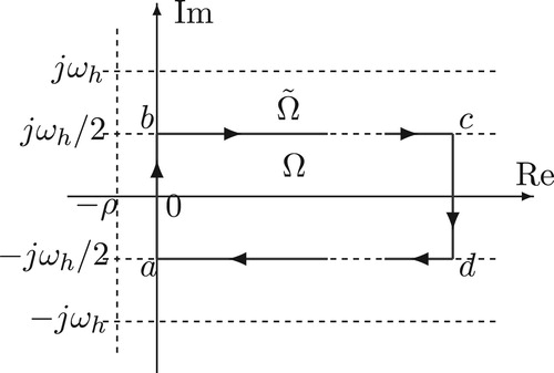Based on these facts, let the Cauchy integral contour be the boundary of the right-half portion of ${\mathbf{C}}_f$, namely the bold-line curve $\tilde{\mathrm{\Omega }}$ in Figure 1, whose interior is denoted by Ω. By Figure 1, we have $\tilde{\mathrm{\Omega }}:={\tilde{\mathrm{\Omega }}}_{ab}\cup {\tilde{\mathrm{\Omega }}}_{bc}\cup {\tilde{\mathrm{\Omega }}}_{cd}\cup {\tilde{\mathrm{\Omega }}}_{da}$ Since $\mathcal{G}\left(s\right)$ may not be well-defined for some $s\in \mathrm{\Lambda }\cap \tilde{\mathrm{\Omega }}$ if $\mathrm{\Lambda }\cap \tilde{\mathrm{\Omega }}$ is not empty (namely, $\mathcal{Q}-\mathcal{E}\left(j0\right)$ has eigenvalues on $\tilde{\mathrm{\Omega }}$), $\tilde{\mathrm{\Omega }}$ must detour these points in $\mathrm{\Lambda }\cap \tilde{\mathrm{\Omega }}$. If $\mathrm{\Lambda }\cap \tilde{\mathrm{\Omega }}$ is not empty, the contour will be slightly shifted as ${\tilde{\mathrm{\Omega }}}_s=:\tilde{\mathrm{\Omega }}+\alpha +j\beta$, where α and β are small constants. Since Λ is the set of isolated points, ${\tilde{\mathrm{\Omega }}}_s$ always exists. In the sequel, we do not specify which contour is meant by $\tilde{\mathrm{\Omega }}$.

As is known by Zhou and Hagiwara (2005), the return difference relation between the open-loop and closed-loop characteristic polynomials is rigorously established and quoted as follows. (8) $\begin{array}{rl}& \frac{{det}_2[\mathcal{I}-{\mathcal{E}}^{-1}(s+\rho \left)\right({\mathcal{A}}_c+\rho \mathcal{I}\left)\right]}{{det}_2[\mathcal{I}-{\mathcal{E}}^{-1}(s+\rho \left)\right(\mathcal{A}+\rho \mathcal{I}\left)\right]}\\ & =\exp \left\{\mathrm{\Delta }\right(s+\rho \left)\right\}{det}_2[\mathcal{I}+\mathcal{K}\mathcal{G}(s\left)\right]\end{array}$(8) where $\mathcal{K}=:\mathcal{T}\left\{K\right(t\left)\right\}$ and (9) $\mathrm{\Delta }(s+\rho )=\mathrm{tr}\left({\mathcal{E}}^{-1}\right(s+\rho \left)\right(\mathcal{A}+\rho \mathcal{I}\left)\right(\mathcal{E}\left(s\right)-\mathcal{A}{)}^{-1}\mathcal{B}\mathcal{K}\mathcal{C})$(9) In (8(8) $\begin{array}{rl}& \frac{{det}_2[\mathcal{I}-{\mathcal{E}}^{-1}(s+\rho \left)\right({\mathcal{A}}_c+\rho \mathcal{I}\left)\right]}{{det}_2[\mathcal{I}-{\mathcal{E}}^{-1}(s+\rho \left)\right(\mathcal{A}+\rho \mathcal{I}\left)\right]}\\ & =\exp \left\{\mathrm{\Delta }\right(s+\rho \left)\right\}{det}_2[\mathcal{I}+\mathcal{K}\mathcal{G}(s\left)\right]\end{array}$(8) ) and (9(9) $\mathrm{\Delta }(s+\rho )=\mathrm{tr}\left({\mathcal{E}}^{-1}\right(s+\rho \left)\right(\mathcal{A}+\rho \mathcal{I}\left)\right(\mathcal{E}\left(s\right)-\mathcal{A}{)}^{-1}\mathcal{B}\mathcal{K}\mathcal{C})$(9) ), $\rho \ge 0$ is introduced to guarantee that ${\mathcal{E}}^{-1}(s+\rho )$ exists when s is running over the imaginary axis portion of the Cauchy contour. Independent of $\rho \ge 0$, the zeros of ${det}_2[\mathcal{I}-{\mathcal{E}}^{-1}(s+\rho \left)\right({\mathcal{A}}_c+\rho \mathcal{I}\left)\right]$ and those of ${det}_2[\mathcal{I}-{\mathcal{E}}^{-1}(s+\rho \left)\right(\mathcal{A}+\rho \mathcal{I}\left)\right]$ are nothing but the zeros of the closed-loop and open-loop characteristic polynomials, respectively.

Figure 1. Cauchy contour for asymptotic stability in LCP systems.

3.2. Complex scaling stability locus

To define the complex scaling locus, we re-write (8(8) $\begin{array}{rl}& \frac{{det}_2[\mathcal{I}-{\mathcal{E}}^{-1}(s+\rho \left)\right({\mathcal{A}}_c+\rho \mathcal{I}\left)\right]}{{det}_2[\mathcal{I}-{\mathcal{E}}^{-1}(s+\rho \left)\right(\mathcal{A}+\rho \mathcal{I}\left)\right]}\\ & =\exp \left\{\mathrm{\Delta }\right(s+\rho \left)\right\}{det}_2[\mathcal{I}+\mathcal{K}\mathcal{G}(s\left)\right]\end{array}$(8) ) as (10) $\begin{array}{rl}& \frac{{det}_2[\mathcal{I}-{\mathcal{E}}^{-1}(s+\rho \left)\right({\mathcal{A}}_c+\rho \mathcal{I}\left)\right]}{\beta (s+\rho )}=f(s,\rho )\\ & =:\frac{{det}_2[\mathcal{I}-{\mathcal{E}}^{-1}(s+\rho \left)\right(\mathcal{A}+\rho \mathcal{I}\left)\right]}{\beta (s+\rho )}\\ & \times \exp \left\{\mathrm{\Delta }\right(s+\rho \left)\right\}{det}_2[\mathcal{I}+\mathcal{K}\mathcal{G}(s\left)\right]\end{array}$(10) Thus, we can re-write the open- and closed-loop characteristic polynomials in (8(8) $\begin{array}{rl}& \frac{{det}_2[\mathcal{I}-{\mathcal{E}}^{-1}(s+\rho \left)\right({\mathcal{A}}_c+\rho \mathcal{I}\left)\right]}{{det}_2[\mathcal{I}-{\mathcal{E}}^{-1}(s+\rho \left)\right(\mathcal{A}+\rho \mathcal{I}\left)\right]}\\ & =\exp \left\{\mathrm{\Delta }\right(s+\rho \left)\right\}{det}_2[\mathcal{I}+\mathcal{K}\mathcal{G}(s\left)\right]\end{array}$(8) ) into a separate fashion with the complex scaling comparator $\beta (s+\rho )$. The comparator satisfies

• $\beta (s+\rho )$ is meromorphic and Hurwitz. Factor cancellations between $\beta (s+\rho )$ and ${det}_2[\mathcal{I}-{\mathcal{E}}^{-1}(s+\rho \left)\right({\mathcal{A}}_c+\rho \mathcal{I}\left)\right]$, if any, are related only to stable eigenvalues.

• $\beta (s+\rho )$ has the same countably infinite many zeros as that of ${det}_2[\mathcal{I}-{\mathcal{E}}^{-1}(s+\rho \left)\right({\mathcal{A}}_c+\rho \mathcal{I}\left)\right]$. This ensures that (10(10) $\begin{array}{rl}& \frac{{det}_2[\mathcal{I}-{\mathcal{E}}^{-1}(s+\rho \left)\right({\mathcal{A}}_c+\rho \mathcal{I}\left)\right]}{\beta (s+\rho )}=f(s,\rho )\\ & =:\frac{{det}_2[\mathcal{I}-{\mathcal{E}}^{-1}(s+\rho \left)\right(\mathcal{A}+\rho \mathcal{I}\left)\right]}{\beta (s+\rho )}\\ & \times \exp \left\{\mathrm{\Delta }\right(s+\rho \left)\right\}{det}_2[\mathcal{I}+\mathcal{K}\mathcal{G}(s\left)\right]\end{array}$(10) ) is numerically bounded so that the corresponding complex scaling locus can be plotted within a bounded area around the origin.

• Zeros of $\beta (s+\rho )$ are $j{\omega }_h$-periodic vertically and of the same distribution pattern as those of ${det}_2[\mathcal{I}-{\mathcal{E}}^{-1}(s+\rho \left)\right({\mathcal{A}}_c+\rho \mathcal{I}\left)\right]$. This is convenient for us to plot the complex scaling locus.

Indeed, we can simply define (11) $\beta (s+\rho )=:{det}_2(\mathcal{I}-{\mathcal{E}}^{-1}(s+\rho \left)\right(\rho \mathcal{I}+\mathcal{T}\left(F\right)\left)\right)$(11) where $F\in {\mathbf{R}}^{n\times n}$ can be any Hurwitz matrix. Obviously, the above conditions are satisfied by this scaling comparator. In the sequel, $\beta (s+\rho )$ of (11(11) $\beta (s+\rho )=:{det}_2(\mathcal{I}-{\mathcal{E}}^{-1}(s+\rho \left)\right(\rho \mathcal{I}+\mathcal{T}\left(F\right)\left)\right)$(11) ) is always meant.

Now, let us see how a complex scaling locus is yielded according to (10(10) $\begin{array}{rl}& \frac{{det}_2[\mathcal{I}-{\mathcal{E}}^{-1}(s+\rho \left)\right({\mathcal{A}}_c+\rho \mathcal{I}\left)\right]}{\beta (s+\rho )}=f(s,\rho )\\ & =:\frac{{det}_2[\mathcal{I}-{\mathcal{E}}^{-1}(s+\rho \left)\right(\mathcal{A}+\rho \mathcal{I}\left)\right]}{\beta (s+\rho )}\\ & \times \exp \left\{\mathrm{\Delta }\right(s+\rho \left)\right\}{det}_2[\mathcal{I}+\mathcal{K}\mathcal{G}(s\left)\right]\end{array}$(10) ) along $\tilde{\mathrm{\Omega }}$. We segment $\tilde{\mathrm{\Omega }}$ into ${\tilde{\mathrm{\Omega }}}_{ab}$, ${\tilde{\mathrm{\Omega }}}_{bc}$, ${\tilde{\mathrm{\Omega }}}_{cd}$ and ${\tilde{\mathrm{\Omega }}}_{da}$ as in Figure 1 and do the following observations.

• Since ${det}_2[\mathcal{I}-{\mathcal{E}}^{-1}(s+\rho \left)\right(\mathcal{A}+\rho \mathcal{I}\left)\right]$, $\beta (s+\rho )$, ${det}_2[\mathcal{I}+\mathcal{K}\mathcal{G}(s\left)\right]$ and $\mathrm{\Delta }(s+\rho )$ are $j{\omega }_h$-periodic conjugate, in the sense that $f(\tilde{s},\rho )=\overline{f(s,\rho )}$ for any $s\in \mathbf{C}$ and $\overline{s}=s-j{\omega }_h$. In particular, for each $s\in {\tilde{\mathrm{\Omega }}}_{bc}$, $\tilde{s}=s-j{\omega }_h\in {\tilde{\mathrm{\Omega }}}_{da}$ such that $\tilde{s}=\overline{s}$. It follows that $f(\tilde{s},\rho )=f(\overline{s},\rho )=\left(f\right(s,\rho ){)}^{\ast }$, where $(\cdot {)}^{\ast }$ denotes the complex conjugate. Hence, the curve portion of $f(s,\rho )$ for $s\in {\tilde{\mathrm{\Omega }}}_{bc}$ and that for $s\in {\tilde{\mathrm{\Omega }}}_{da}$ are symmetric with respect to the real axis.

• If $\mathrm{Re}\left(s\right)>0$ is large enough for each $s\in {\tilde{\mathrm{\Omega }}}_{cd}$, then $f(s,\rho )\to \underset{s\to \mathrm{\infty }}{lim}{det}_2[\mathcal{I}+\mathcal{K}\mathcal{G}(s\left)\right]$.

In summary, the locus $f(s,\rho ):{\tilde{\mathrm{\Omega }}}_{da}\cup {\tilde{\mathrm{\Omega }}}_{ab}\cup {\tilde{\mathrm{\Omega }}}_{bc}\to \mathbf{C}$ forms a closed curve. To investigate its encirclement around the origin with respect to the whole $\tilde{\mathrm{\Omega }}$, it is enough to see only the segments corresponding to ${\tilde{\mathrm{\Omega }}}_{ab}$, ${\tilde{\mathrm{\Omega }}}_{cd}$ and ${\tilde{\mathrm{\Omega }}}_{da}$. In the sequel, the closed curve of piecing together the segments corresponding to ${\tilde{\mathrm{\Omega }}}_{bc}$, ${\tilde{\mathrm{\Omega }}}_{cd}$ and ${\tilde{\mathrm{\Omega }}}_{da}$ is called the complex scaling locus.

3.3. Complex scaling stability criterion

Now we are ready to state and show the complex scaling stability criterion.

Theorem 3.1

Assume that $A\left(t\right),B\left(t\right),C\left(t\right)$ of the LCP system (1(1) $G:\{\begin{array}{l}\dot{x}=A\left(t\right)x+B\left(t\right)u\\ y=C\left(t\right)x\end{array}$(1) ) and the feedback matrix $K\left(t\right)$ belong to $L_{\mathrm{AC}}[0,h]\cap L_{\mathrm{PCD}}[0,h]$. Then, the closed-loop system (6(6) $G_c:\{\begin{array}{l}\dot{x}=A_c\left(t\right)x+B\left(t\right)v\\ y=C\left(t\right)x\end{array}$(6) ) is asymptotically stable if and only if the complex scaling locus $f(s,\rho ):\check{\mathrm{\Omega }}\to \mathbf{C}$, or simply $f(s,\rho ){|}_{s\in \check{\mathrm{\Omega }}}$, vanishes nowhere over $s\in \check{\mathrm{\Omega }}$, and the number of the clockwise encirclements around the origin is equal to that of the counter-clockwise encirclements around the origin. In the above, $f(s,\rho )$ and $\beta (s+\rho )$ are defined in (10(10) $\begin{array}{rl}& \frac{{det}_2[\mathcal{I}-{\mathcal{E}}^{-1}(s+\rho \left)\right({\mathcal{A}}_c+\rho \mathcal{I}\left)\right]}{\beta (s+\rho )}=f(s,\rho )\\ & =:\frac{{det}_2[\mathcal{I}-{\mathcal{E}}^{-1}(s+\rho \left)\right(\mathcal{A}+\rho \mathcal{I}\left)\right]}{\beta (s+\rho )}\\ & \times \exp \left\{\mathrm{\Delta }\right(s+\rho \left)\right\}{det}_2[\mathcal{I}+\mathcal{K}\mathcal{G}(s\left)\right]\end{array}$(10) ) and (11(11) $\beta (s+\rho )=:{det}_2(\mathcal{I}-{\mathcal{E}}^{-1}(s+\rho \left)\right(\rho \mathcal{I}+\mathcal{T}\left(F\right)\left)\right)$(11) ), respectively, and $\check{\mathrm{\Omega }}:={\tilde{\mathrm{\Omega }}}_{da}\cup {\tilde{\mathrm{\Omega }}}_{ab}\cup {\tilde{\mathrm{\Omega }}}_{bc}$.

Proof.

Apply the argument principle (Stein & Shakarchi, 2003, p. 90) to (10(10) $\begin{array}{rl}& \frac{{det}_2[\mathcal{I}-{\mathcal{E}}^{-1}(s+\rho \left)\right({\mathcal{A}}_c+\rho \mathcal{I}\left)\right]}{\beta (s+\rho )}=f(s,\rho )\\ & =:\frac{{det}_2[\mathcal{I}-{\mathcal{E}}^{-1}(s+\rho \left)\right(\mathcal{A}+\rho \mathcal{I}\left)\right]}{\beta (s+\rho )}\\ & \times \exp \left\{\mathrm{\Delta }\right(s+\rho \left)\right\}{det}_2[\mathcal{I}+\mathcal{K}\mathcal{G}(s\left)\right]\end{array}$(10) ). It follows that (12) $\begin{array}{rl}& Z(\frac{{det}_2[\mathcal{I}-{\mathcal{E}}^{-1}(s+\rho \left)\right({\mathcal{A}}_c+\rho \mathcal{I}\left)\right]}{\beta (s+\rho )})\\ & -P(\frac{{det}_2[\mathcal{I}-{\mathcal{E}}^{-1}(s+\rho \left)\right({\mathcal{A}}_c+\rho \mathcal{I}\left)\right]}{\beta (s+\rho )})\\ & =n_c\left(f\right(s,\rho \left){|}_{s\in \check{\mathrm{\Omega }}}\right)-n_{\overline{c}}\left(f\right(s,\rho \left){|}_{s\in \check{\mathrm{\Omega }}}\right)\end{array}$(12) where $Z(\cdot )$ and $P(\cdot )$ denote the zeros and poles numbers of $(\cdot )$, respectively, in Ω, while $n_c(\cdot )$ and $n_{\overline{c}}(\cdot )$ mean the clockwise and counter-clockwise encirclement numbers of a locus $(\cdot )$, respectively.

Further, by the definitions of $\beta (s+\rho )$ and ${det}_2[\mathcal{I}-{\mathcal{E}}^{-1}(s+\rho \left)\right({\mathcal{A}}_c+\rho \mathcal{I}\left)\right]$, they have the same denominator polynomial, which is the nominator of $\beta (s+\rho )$. Hence, it is easy to see that (13) $\{\begin{array}{l}P\left({det}_2\right[\mathcal{I}-{\mathcal{E}}^{-1}(s+\rho )({\mathcal{A}}_c+\rho \mathcal{I})\left]\right)=P\left(\beta \right(s+\rho \left)\right)\\ Z\left(\beta (s+\rho )\right)=0\end{array}$(13) and (14) $\{\begin{array}{l}Z\left(\frac{{det}_2[\mathcal{I}-{\mathcal{E}}^{-1}(s+\rho \left)\right({\mathcal{A}}_c+\rho \mathcal{I}\left)\right]}{\beta (s+\rho )}\right)\\ =Z({det}_2[\mathcal{I}-{\mathcal{E}}^{-1}(s+\rho \left)\right({\mathcal{A}}_c+\rho \mathcal{I}\left)\right])\\ P\left(\frac{{det}_2[\mathcal{I}-{\mathcal{E}}^{-1}(s+\rho \left)\right({\mathcal{A}}_c+\rho \mathcal{I}\left)\right]}{\beta (s+\rho )}\right)\\ =Z\left(\beta \right(s+\rho \left)\right)=0\end{array}$(14) The relations in (14(14) $\{\begin{array}{l}Z\left(\frac{{det}_2[\mathcal{I}-{\mathcal{E}}^{-1}(s+\rho \left)\right({\mathcal{A}}_c+\rho \mathcal{I}\left)\right]}{\beta (s+\rho )}\right)\\ =Z({det}_2[\mathcal{I}-{\mathcal{E}}^{-1}(s+\rho \left)\right({\mathcal{A}}_c+\rho \mathcal{I}\left)\right])\\ P\left(\frac{{det}_2[\mathcal{I}-{\mathcal{E}}^{-1}(s+\rho \left)\right({\mathcal{A}}_c+\rho \mathcal{I}\left)\right]}{\beta (s+\rho )}\right)\\ =Z\left(\beta \right(s+\rho \left)\right)=0\end{array}$(14) ) must be interpreted before removing all reducible factors between $\beta (s+\rho )$ and ${det}_2[\mathcal{I}-{\mathcal{E}}^{-1}(s+\rho \left)\right({\mathcal{A}}_c+\rho \mathcal{I}\left)\right]$ as appropriately.

Substituting the above results for (12(12) $\begin{array}{rl}& Z(\frac{{det}_2[\mathcal{I}-{\mathcal{E}}^{-1}(s+\rho \left)\right({\mathcal{A}}_c+\rho \mathcal{I}\left)\right]}{\beta (s+\rho )})\\ & -P(\frac{{det}_2[\mathcal{I}-{\mathcal{E}}^{-1}(s+\rho \left)\right({\mathcal{A}}_c+\rho \mathcal{I}\left)\right]}{\beta (s+\rho )})\\ & =n_c\left(f\right(s,\rho \left){|}_{s\in \check{\mathrm{\Omega }}}\right)-n_{\overline{c}}\left(f\right(s,\rho \left){|}_{s\in \check{\mathrm{\Omega }}}\right)\end{array}$(12) ), we can write (15) $\begin{array}{rl}& Z\left({det}_2\right[\mathcal{I}-{\mathcal{E}}^{-1}(s+\rho )({\mathcal{A}}_c+\rho \mathcal{I})\left]\right)\\ & =n_c\left(f\right(s,\rho \left){|}_{s\in \check{\mathrm{\Omega }}}\right)-n_{\overline{c}}\left(f\right(s,\rho \left){|}_{s\in \check{\mathrm{\Omega }}}\right)\end{array}$(15) It follows immediately that if $n_c(\cdot )=n_{\overline{c}}(\cdot )$, and thus $Z\left({det}_2\right[\mathcal{I}-{\mathcal{E}}^{-1}(s+\rho )({\mathcal{A}}_c+\rho \mathcal{I})\left]\right)=0$. This tells us exactly that the closed-loop LCP system has no poles in Ω. This leads to asymptotical stability, and the sufficiency is proved.

To see the necessity, assume that the closed-loop system is asymptotically stable. Thus, $Z\left({det}_2\right[\mathcal{I}-{\mathcal{E}}^{-1}(s+\rho )({\mathcal{A}}_c+\rho \mathcal{I})\left]\right)=0$. Based on (14(14) $\{\begin{array}{l}Z\left(\frac{{det}_2[\mathcal{I}-{\mathcal{E}}^{-1}(s+\rho \left)\right({\mathcal{A}}_c+\rho \mathcal{I}\left)\right]}{\beta (s+\rho )}\right)\\ =Z({det}_2[\mathcal{I}-{\mathcal{E}}^{-1}(s+\rho \left)\right({\mathcal{A}}_c+\rho \mathcal{I}\left)\right])\\ P\left(\frac{{det}_2[\mathcal{I}-{\mathcal{E}}^{-1}(s+\rho \left)\right({\mathcal{A}}_c+\rho \mathcal{I}\left)\right]}{\beta (s+\rho )}\right)\\ =Z\left(\beta \right(s+\rho \left)\right)=0\end{array}$(14) ) and (15(15) $\begin{array}{rl}& Z\left({det}_2\right[\mathcal{I}-{\mathcal{E}}^{-1}(s+\rho )({\mathcal{A}}_c+\rho \mathcal{I})\left]\right)\\ & =n_c\left(f\right(s,\rho \left){|}_{s\in \check{\mathrm{\Omega }}}\right)-n_{\overline{c}}\left(f\right(s,\rho \left){|}_{s\in \check{\mathrm{\Omega }}}\right)\end{array}$(15) ), we notice that $0=n_c\left(f\right(s,\rho \left){|}_{s\in \check{\mathrm{\Omega }}}\right)-n_{\overline{c}}\left(f\right(s,\rho \left){|}_{s\in \check{\mathrm{\Omega }}}\right)$, which says that the complex scaling locus has the same clockwise and counter-clockwise encirclements around the origin. This accomplishes the proof.

Some remarks about Theorem 3.1:

• Clearly, the complex scaling 2-regularised determinant return difference relation (10(10) $\begin{array}{rl}& \frac{{det}_2[\mathcal{I}-{\mathcal{E}}^{-1}(s+\rho \left)\right({\mathcal{A}}_c+\rho \mathcal{I}\left)\right]}{\beta (s+\rho )}=f(s,\rho )\\ & =:\frac{{det}_2[\mathcal{I}-{\mathcal{E}}^{-1}(s+\rho \left)\right(\mathcal{A}+\rho \mathcal{I}\left)\right]}{\beta (s+\rho )}\\ & \times \exp \left\{\mathrm{\Delta }\right(s+\rho \left)\right\}{det}_2[\mathcal{I}+\mathcal{K}\mathcal{G}(s\left)\right]\end{array}$(10) ) is expressed still in terms of the open-loop and closed-loop modified harmonic state operators. However, when applying the argument principle to (10(10) $\begin{array}{rl}& \frac{{det}_2[\mathcal{I}-{\mathcal{E}}^{-1}(s+\rho \left)\right({\mathcal{A}}_c+\rho \mathcal{I}\left)\right]}{\beta (s+\rho )}=f(s,\rho )\\ & =:\frac{{det}_2[\mathcal{I}-{\mathcal{E}}^{-1}(s+\rho \left)\right(\mathcal{A}+\rho \mathcal{I}\left)\right]}{\beta (s+\rho )}\\ & \times \exp \left\{\mathrm{\Delta }\right(s+\rho \left)\right\}{det}_2[\mathcal{I}+\mathcal{K}\mathcal{G}(s\left)\right]\end{array}$(10) ), we no longer need to check whether ${det}_2[\mathcal{I}-{\mathcal{E}}^{-1}(s+\rho \left)\right(\mathcal{A}+\rho \mathcal{I}\left)\right]$ has any zeros in Ω.

• Reducible factors between ${det}_2[\mathcal{I}-{\mathcal{E}}^{-1}(s+\rho \left)\right({\mathcal{A}}_c+\rho \mathcal{I}\left)\right]$ and $\beta (s+\rho )$ exist, if the LCP system is uncontrollable and/or unobservable (Zhou et al., 2016). Factor cancellations do not affect our zeros distribution testing of ${det}_2[\mathcal{I}-{\mathcal{E}}^{-1}(s+\rho \left)\right({\mathcal{A}}_c+\rho \mathcal{I}\left)\right]$ since $\beta (s+\rho )$ is Hurwitz.

• Stability in Theorem 3.1 is meant in asymptotical stability. If the state decreasing ratio is examined, the conditions should be interpreted in exponential stability. It is simple to see that such stability analysis can be achieved by replacing the contour $\check{\mathrm{\Omega }}$ with some ε-shifted one, that is $\check{\mathrm{\Omega }}-ϵ$. with $ϵ>0$ being an expected decreasing ratio.

4. Finite-dimensional versions of Theorem 3.1

Since the 2-regularised determinant and trace of infinite dimensionality operators are involved, we must consider how to implement Theorem 3.1 by operator matrix truncations. Then, stability analysis is reduced to that of finite-dimensional LTI systems.

4.1. Two-step truncation on Toeplitz operators

Firstly, let us truncate $\mathcal{A}$ to ${\mathcal{A}}_{[N,M]}:=\mathrm{diag}[\cdots ,A_{NM},A_{NM},A_{NM},\dots ]$ with $M\ge N+1$ and (16) $\begin{array}{r}{A}_{NM}=\left[\begin{array}{ccccc}{A}_0& \cdots & A_{-N}& & 0\\ ⋮& \ddots & & \ddots & \\ A_N& \cdots & A_0& \cdots & A_{-N}\\ & \ddots & & \ddots & ⋮\\ 0& & A_N& \cdots & A_0\end{array}\right]\in {\mathbf{C}}^{(2M+1)n\times (2M+1)n}\end{array}$(16) We similarly define ${\mathcal{B}}_{[N,M]}$ (resp., $B_{NM}$), ${\mathcal{C}}_{[N,M]}$ (resp., $C_{NM}$) and ${\mathcal{K}}_{[N,M]}$ (resp., $K_{NM}$)

Secondly, based on the two-step truncation, $\mathcal{G}\left(s\right)=\mathcal{C}\left(\mathcal{E}\right(s)-\mathcal{A}{)}^{-1}\mathcal{B}$ is approximated by (17) $\begin{array}{rl}{\mathcal{G}}_{[N,M]}\left(j\varphi \right)& =\text{block diag}\\ & \times [\cdots ,G_{-1NM}(s),G_{0NM}(s),G_{1NM}(s),\dots ]\end{array}$(17) where (18) $G_{mNM}\left(s\right):=C_{NM}\left(E_{mM}\right(s)-A_{NM}{)}^{-1}{B}_{NM},m\in \mathbf{Z}$(18) with $E_{mM}\left(s\right)=\text{diag}\left[{\varphi }_{m(2M+1)-M}\right(s)I,\dots ,{\varphi }_{m(2M+1)+M}(s\left)I\right]$.

Finally, we apply the two-step truncation on $\mathrm{\Delta }(s+\rho )$ to obtain (19) ${\mathrm{\Delta }}_{[N,M]}(s+\rho )=:-{\mathrm{\Sigma }}_m\mathrm{tr}\left({\mathrm{\Delta }}_{mNM}\right(s+\rho \left)\right)$(19) where (20) $\begin{array}{rl}{\mathrm{\Delta }}_{mNM}(s+\rho )& :=E_{mM}^{-1}(s+\rho )(A_{NM}+\rho I_M)\\ & \times \left(E_{mM}\right(s)-A_{NM}{)}^{-1}{B}_{NM}{K}_{NM}{C}_{NM}\end{array}$(20)

4.2. Convergence lemma about the two-step truncation

We collect convergence relations for the two-step truncations in the 2-regularised determinant and trace, which can be shown by the proof techniques in Zhou and Hagiwara (2005).

Lemma 4.1

Assume in the FDLCP system (1(1) $G:\{\begin{array}{l}\dot{x}=A\left(t\right)x+B\left(t\right)u\\ y=C\left(t\right)x\end{array}$(1) ) that $A\left(t\right)\in L_{\mathrm{PCD}}[0,h]$ and $B\left(t\right),C\left(t\right)\in L_{\mathrm{AC}}[0,h]$, and the domain $\mathrm{\Omega }\subset \mathbf{C}$ satisfies (A1). Then for any $\mu >0$ and each fixed N>0, there exists an integer $M_0(N,\mu )>0$ such that for all $M\ge M_0(N,\mu )$ and uniformly over $s\in \tilde{\mathrm{\Omega }}$, it holds $\begin{array}{r}\{\begin{array}{l}|{det}_2[\underset{\_}{I}+{\underset{\_}{K}}_{[N,M]}{\underset{\_}{G}}_{[N,M]}(s\left)\right]-{det}_2[\underset{\_}{I}+{\underset{\_}{K}}_{\left[N\right]}{\underset{\_}{G}}_{\left[N\right]}(s\left)\right]|<\mu \\ |{det}_2[\underset{\_}{I}-{\underset{\_}{E}}^{-1}(s+\rho \left)\right({\underset{\_}{A}}_{[N,M]}+\rho \underset{\_}{I}\left)\right]\\ -{det}_2[\underset{\_}{I}-{\underset{\_}{E}}^{-1}(s+\rho \left)\right({\underset{\_}{A}}_{\left[N\right]}+\rho \underset{\_}{I}\left)\right]|<\mu \\ |{\mathrm{\Delta }}_{[N,M]}(s+\rho )-\mathrm{\Delta }(s+\rho )|<\mu \end{array}\end{array}$

Now we show that the truncated version can actually be reduced to finite-dimensional computations with convergence being ensured. Indeed, by definition, we have (21) $\begin{array}{rl}& \frac{{det}_2[\underset{\_}{I}-{\underset{\_}{E}}_{[N,M]}^{-1}(s+\rho \left)\right({\underset{\_}{A}}_{[N,M]}+\rho \underset{\_}{I}\left)\right]}{{\beta }_{\left[M\right]}(s+\rho )}\\ & \cdot \exp \left\{{\mathrm{\Delta }}_{[N,M]}\right(s+\rho \left)\right\}{det}_2[\underset{\_}{I}+{\underset{\_}{K}}_{[N,M]}{\underset{\_}{G}}_{[N,M]}(s\left)\right]\\ & ={\prod }_m{\prod }_k(1-{\lambda }_k(E_{mM}^{-1}(s+\rho )(A_{NM}+\rho I_M)\left)\right)\\ & \cdot \exp \left\{{\lambda }_k\right(E_{mM}^{-1}(s+\rho )(A_{NM}+\rho I_M)\left)\right\}\\ & \times \frac{\exp \left\{\sum _m\mathrm{tr}\right({\mathrm{\Delta }}_{mNM}(s+\rho )\left)\right\}}{{\beta }_{\left[M\right]}(s+\rho )}\\ & \cdot {\prod }_m{\prod }_k(1+{\lambda }_k(K_{NM}{G}_{mNM}\left(s\right)\left)\right)\\ & \times \exp \{-{\lambda }_k(K_{NM}{G}_{mNM}\left(s\right)\left)\right\}\end{array}$(21) where ${\beta }_{\left[M\right]}(s+\rho )=:{\prod }_m{c}_{mM}(s+\rho )=\beta (s+\rho )$ in which $c_{mM}(s+\rho )=:{det}_2(I_M-E_{mM}^{-1}(s+\rho \left)\right(\rho I_M+F_M\left)\right))$.

Under the assumptions of Lemma 4.1, for any fixed N>0, it holds uniformly over $s\in \tilde{\mathrm{\Omega }}$ that $\begin{array}{r}\{\begin{array}{l}\underset{M\to \mathrm{\infty }}{lim}\prod _{m\ne 0}{c}_{mM}(s+\rho )=1\\ \underset{M\to \mathrm{\infty }}{lim}\sum _{m\ne 0}\mathrm{tr}\left({\mathrm{\Delta }}_{mNM}\right(s+\rho \left)\right)=0\\ \underset{M\to \mathrm{\infty }}{lim}\prod _{m\ne 0}\prod _k(1-{\lambda }_k(E_{mM}^{-1}(s+\rho )(A_{NM}+\rho I_M)\left)\right)\\ \cdot \exp \left\{{\lambda }_k\right(E_{mM}^{-1}(s+\rho )(A_{NM}+\rho I_M)\left)\right\}=1\\ \underset{M\to \mathrm{\infty }}{lim}\prod _{m\ne 0}\prod _k(1+{\lambda }_k(K_{NM}{G}_{mNM}\left(s\right)\left)\right)\\ \cdot \exp \{-{\lambda }_k(K_{NM}{G}_{mNM}\left(s\right)\left)\right\}=1\end{array}\end{array}$ The above convergence relations, together with (21(21) $\begin{array}{rl}& \frac{{det}_2[\underset{\_}{I}-{\underset{\_}{E}}_{[N,M]}^{-1}(s+\rho \left)\right({\underset{\_}{A}}_{[N,M]}+\rho \underset{\_}{I}\left)\right]}{{\beta }_{\left[M\right]}(s+\rho )}\\ & \cdot \exp \left\{{\mathrm{\Delta }}_{[N,M]}\right(s+\rho \left)\right\}{det}_2[\underset{\_}{I}+{\underset{\_}{K}}_{[N,M]}{\underset{\_}{G}}_{[N,M]}(s\left)\right]\\ & ={\prod }_m{\prod }_k(1-{\lambda }_k(E_{mM}^{-1}(s+\rho )(A_{NM}+\rho I_M)\left)\right)\\ & \cdot \exp \left\{{\lambda }_k\right(E_{mM}^{-1}(s+\rho )(A_{NM}+\rho I_M)\left)\right\}\\ & \times \frac{\exp \left\{\sum _m\mathrm{tr}\right({\mathrm{\Delta }}_{mNM}(s+\rho )\left)\right\}}{{\beta }_{\left[M\right]}(s+\rho )}\\ & \cdot {\prod }_m{\prod }_k(1+{\lambda }_k(K_{NM}{G}_{mNM}\left(s\right)\left)\right)\\ & \times \exp \{-{\lambda }_k(K_{NM}{G}_{mNM}\left(s\right)\left)\right\}\end{array}$(21) ), imply that for any $\mu >0$ sufficiently small and fixed N>0 sufficiently large, it holds as $M\to \mathrm{\infty }$ that (22) $\begin{array}{rl}& |\frac{{det}_2[I_M-E_{0NM}^{-1}(s+\rho \left)\right(A_{NM}+\rho I_M\left)\right]}{{\beta }_{0,M}(s+\rho )}\\ & \cdot \exp \left\{{\mathrm{\Delta }}_{0NM}\right(s+\rho \left)\right\}{det}_2[I_M+K_{NM}{G}_{0NM}(s\left)\right]\\ & -\frac{{det}_2[\underset{\_}{I}-{\underset{\_}{E}}^{-1}(s+\rho \left)\right(\underset{\_}{A}+\rho \underset{\_}{I}\left)\right]}{}\\ & \cdot \beta (s+\rho )\exp \left\{\mathrm{\Delta }\right(s+\rho \left)\right\}{det}_2[\underset{\_}{I}+\underset{\_}{K}\underset{\_}{G}(s\left)\right]|<\mu \end{array}$(22)

4.3. Finite-dimensional complex scaling stability criterion

Summarizing the above discussions, we are led to the following theorem, which reduces the infinite-dimensional criterion of Theorem 3.1 to a finite-dimensional version.

Theorem 4.1

Suppose in the LCP system (1(1) $G:\{\begin{array}{l}\dot{x}=A\left(t\right)x+B\left(t\right)u\\ y=C\left(t\right)x\end{array}$(1) ) that $A\left(t\right)$, $B\left(t\right)$, $C\left(t\right)\in L_{\mathrm{AC}}[0,h]\cap L_{\mathrm{PCD}}[0,h]$. Let the feedback matrix $K\left(t\right)$ belong to $L_{\mathrm{AC}}[0,h]\cap L_{\mathrm{PCD}}[0,h]$. Then, the closed-loop system (6(6) $G_c:\{\begin{array}{l}\dot{x}=A_c\left(t\right)x+B\left(t\right)v\\ y=C\left(t\right)x\end{array}$(6) ) is asymptotically stable if and only if there exist sufficiently large integers N>0 and $M\ge N+1$ such that the finite-dimensional complex scaling locus (23) $\begin{array}{rl}& f(s,\rho ,M,N){|}_{s\in \check{\mathrm{\Omega }}}\\ & =:\frac{{det}_2[I_M-E_{0NM}^{-1}(s+\rho \left)\right(A_{NM}+\rho I_M\left)\right]}{{\beta }_{0,M}(s+\rho )}\\ & \cdot \exp \left\{{\mathrm{\Delta }}_{0NM}\right(s+\rho \left)\right\}{det}_2[I_M+K_{NM}{G}_{0NM}(s\left)\right]:\check{\mathrm{\Omega }}\to \mathbf{C}\end{array}$(23) vanishes nowhere over $s\in \check{\mathrm{\Omega }}$, and the number of the clockwise encirclements around the origin is equal to that of the counter-clockwise encirclements.

In the above, $\rho >0$ is arbitrarily taken, and $G_{0NM}\left(s\right)$ and ${\mathrm{\Delta }}_{0NM}(s+\rho )$ are defined in (18(18) $G_{mNM}\left(s\right):=C_{NM}\left(E_{mM}\right(s)-A_{NM}{)}^{-1}{B}_{NM},m\in \mathbf{Z}$(18) ) and (20(20) $\begin{array}{rl}{\mathrm{\Delta }}_{mNM}(s+\rho )& :=E_{mM}^{-1}(s+\rho )(A_{NM}+\rho I_M)\\ & \times \left(E_{mM}\right(s)-A_{NM}{)}^{-1}{B}_{NM}{K}_{NM}{C}_{NM}\end{array}$(20) ), respectively, with m=0. Also (24) ${\beta }_{0,M}(s+\rho )=:{det}_2(I_M-E_{0,M}^{-1}(s+\rho \left)\right(\rho I_M+F_M\left)\right)$(24) where $F_M=\mathrm{diag}[F,F,\dots ,F]\in {\mathbf{C}}^{n(2M+1)\times n(2M+1)}$ with $F\in {\mathbf{C}}^{n\times n}$ being some arbitrary Hurwitz matrix, and $I_M$ is the $n(2M+1)\times n(2M+1)$ identity matrix. $\check{\mathrm{\Omega }}$ is defined in Theorem 3.1.

Proof.

The stability assertion follows from Theorem 3.1 if we notice the truncation convergence is guaranteed when N>0 and $M\ge N+1$ are sufficiently large by Lemma 4.1. This gives the convergence properties between the infinite- and finite-dimensional complex scaling loci as in (22(22) $\begin{array}{rl}& |\frac{{det}_2[I_M-E_{0NM}^{-1}(s+\rho \left)\right(A_{NM}+\rho I_M\left)\right]}{{\beta }_{0,M}(s+\rho )}\\ & \cdot \exp \left\{{\mathrm{\Delta }}_{0NM}\right(s+\rho \left)\right\}{det}_2[I_M+K_{NM}{G}_{0NM}(s\left)\right]\\ & -\frac{{det}_2[\underset{\_}{I}-{\underset{\_}{E}}^{-1}(s+\rho \left)\right(\underset{\_}{A}+\rho \underset{\_}{I}\left)\right]}{}\\ & \cdot \beta (s+\rho )\exp \left\{\mathrm{\Delta }\right(s+\rho \left)\right\}{det}_2[\underset{\_}{I}+\underset{\_}{K}\underset{\_}{G}(s\left)\right]|<\mu \end{array}$(22) ). From this, we can assert that the finite-dimensional complex scaling locus defined by (23(23) $\begin{array}{rl}& f(s,\rho ,M,N){|}_{s\in \check{\mathrm{\Omega }}}\\ & =:\frac{{det}_2[I_M-E_{0NM}^{-1}(s+\rho \left)\right(A_{NM}+\rho I_M\left)\right]}{{\beta }_{0,M}(s+\rho )}\\ & \cdot \exp \left\{{\mathrm{\Delta }}_{0NM}\right(s+\rho \left)\right\}{det}_2[I_M+K_{NM}{G}_{0NM}(s\left)\right]:\check{\mathrm{\Omega }}\to \mathbf{C}\end{array}$(23) ) must lie in a narrow neighbourhood along the infinite-dimensional complex scaling locus of Theorem 3.1. This in turn implies that the finite-dimensional locus vanishes nowhere, and has the same number of clockwise and counter-clockwise encirclements around the origin of the complex plane, if and only if the infinite-dimensional one does so. Based on this and applying the argument principle to $f(s,\rho ,M,N)$ along $s\in \check{\mathrm{\Omega }}$, together with the fact that the comparator $\beta (s+\rho )$ have no eigenvalues in Ω, we can say that the closed-loop characteristic polynomial ${det}_2[\mathcal{I}-{\mathcal{E}}^{-1}(s\left){\mathcal{A}}_c\right]$ has no eigenvalues in Ω, either. Thus, asymptotic stability in the closed-loop system is confirmed.

Some remarks about Theorem 4.1:

• Since no open-loop poles are involved, the stability conditions can be implemented without locus plotting. That is, we can implement the criterion by computing the argument incremental $\mathrm{\nabla \angle }f(s,\rho ,M,N){|}_{s\in \check{\mathrm{\Omega }}}$ of $f(s,\rho ,M,N)$ along $\check{\mathrm{\Omega }}$ and checking if $|\mathrm{\nabla \angle }f(s,\rho ,M,N){|}_{s\in \check{\mathrm{\Omega }}}|\le \eta$ (where $\eta >0$ is a small number as tolerance error).

5. Stabilization in LCP systems

In this section, we propose several design algorithms in term of static state feedback for stabilising LCP systems that have h-periodic state matrices but the input matrices are constant. That is, we consider the following LCP system (25) $\dot{x}\left(t\right)=A\left(t\right)x\left(t\right)+B_{0}u\left(t\right)$(25) where $A\left(t\right)\in {\mathbf{R}}^{n\times n}$ is h-periodic and $B_0\in {\mathbf{R}}^{n\times m}$ is constant. To (25(25) $\dot{x}\left(t\right)=A\left(t\right)x\left(t\right)+B_{0}u\left(t\right)$(25) ), we introduce a state feedback (26) $u\left(t\right)=-K_{0}x\left(t\right)+v\left(t\right)$(26) where $K_0\in {\mathbf{R}}^{m\times n}$ is constant and $v\left(t\right)$ is a new reference. The closed-loop LCP system is (27) $\dot{x}\left(t\right)=\left(A\right(t)-B_0{K}_0)x\left(t\right)+B_{0}v\left(t\right)$(27) Our problem hereafter is: fix possible constant feedback gain matrix $K_0$ such that the closed-loop LCP system is asymptotically stable.

5.1. Stabilization design via the complex scaling approach

To facilitate our statements, let us define the closed-loop characteristic polynomial as $\begin{array}{rl}{p}_c(s+\rho )& ={det}_2(\mathcal{I}-{\mathcal{E}}^{-1}(s+\rho \left)\right[\mathcal{A}+\rho \mathcal{I}-{\mathcal{B}}_0{\mathcal{K}}_0\left]\right)\\ & ={det}_2(\mathcal{I}-{\mathcal{E}}^{-1}(s+\rho \left)\right[\stackrel{\mathcal{ˆ}}{\mathcal{A}}+{\mathcal{A}}_0+\rho \mathcal{I}-{\mathcal{B}}_0{\mathcal{K}}_0\left]\right)\end{array}$ where ${\mathcal{A}}_0=:\mathcal{T}\left\{A_0\right\}$, ${\mathcal{B}}_0=:\mathcal{T}\left\{B_0\right\}$ and ${\mathcal{K}}_0=:\mathcal{T}\left\{B_0\right\}$, while $\hat{\mathcal{A}}=:\mathcal{T}\left\{{\mathrm{\Sigma }}_{i=-\mathrm{\infty },i\ne 0}^{\mathrm{\infty }}{A}_i{e}^{ji{\omega }_{h}t}\right\}$; that is, $\hat{\mathcal{A}}$ is the infinite- dimensional matrix after removing all the block-diagonal terms from $\mathcal{A}$. Let us write $A_{c,0}=A_0-B_0{K}_0$ and then we observe that $\begin{array}{rl}& p_c(s+\rho )\\ & =:{det}_2\{\mathcal{I}-{\mathcal{E}}^{-1}(s+\rho \left)\right[\rho \mathcal{I}+{\mathcal{A}}_0]-{\mathcal{E}}^{-1}(s+\rho \left)\stackrel{\mathcal{ˆ}}{\mathcal{A}}\right\}\\ & ={det}_2\left\{\right(\mathcal{I}-{\mathcal{E}}^{-1}(s+\rho )[\rho \mathcal{I}+{\mathcal{A}}_0])\\ & \cdot (\mathcal{I}-(\mathcal{E}(s+\rho )-[\rho \mathcal{I}+{\mathcal{A}}_0]{)}^{-1}\stackrel{\mathcal{ˆ}}{\mathcal{A}}\left)\right\}\\ & ={det}_2\left\{\right(\mathcal{I}-{\mathcal{E}}^{-1}(s+\rho )[\rho \mathcal{I}+{\mathcal{A}}_0]\left)\right(\mathcal{I}-\left(\mathcal{E}\right(s)-{\mathcal{A}}_{c,0}{)}^{-1}\stackrel{\mathcal{ˆ}}{\mathcal{A}})\}\\ & ={det}_2\{\mathcal{I}-{\mathcal{E}}^{-1}(s+\rho \left)\right[\rho \mathcal{I}+{\mathcal{A}}_0\left]\right\}{det}_2\{\mathcal{I}-(\mathcal{E}\left(s\right)-{\mathcal{A}}_{c,0}{)}^{-1}\stackrel{\mathcal{ˆ}}{\mathcal{A}}\}\\ & \cdot \exp \left\{\mathrm{tr}\right({\mathcal{E}}^{-1}(s+\rho )[\rho \mathcal{I}+{\mathcal{A}}_0]\left(\mathcal{E}\right(s)-{\mathcal{A}}_{c,0}{)}^{-1}\stackrel{\mathcal{ˆ}}{\mathcal{A}})\}\\ & ={det}_2\{\mathcal{I}-{\mathcal{E}}^{-1}(s+\rho \left)\right[\rho \mathcal{I}+{\mathcal{A}}_0\left]\right\}{det}_2\{\mathcal{I}-(\mathcal{E}\left(s\right)-{\mathcal{A}}_{c,0}{)}^{-1}\stackrel{\mathcal{ˆ}}{\mathcal{A}}\}\end{array}$ The last equation follows from the fact that ${\mathcal{E}}^{-1}(s+\rho )[\rho \mathcal{I}+{\mathcal{A}}_0]\left(\mathcal{E}\right(s)-{\mathcal{A}}_{c,0}{)}^{-1}$ is block-diagonal, and all the diagonal blocks in $\hat{\mathcal{A}}$ are zero. Then, $\mathrm{tr}\left({\mathcal{E}}^{-1}\right(s+\rho \left)\right[\rho \mathcal{I}+{\mathcal{A}}_0\left]\right(\mathcal{E}\left(s\right)-{\mathcal{A}}_{c,0}{)}^{-1}\hat{\mathcal{A}})=0$.

Now let us further choose the complex scaling comparator (28) $\beta (s+\rho )={det}_2\{\mathcal{I}-{\mathcal{E}}^{-1}(s+\rho \left)\right[\rho \mathcal{I}+{\mathcal{A}}_0\left]\right\}$(28) where is a Hurwitz polynomial if all the eigenvalues of $A_0-B_0{K}_0$ can be assigned to have negative real parts by choosing $K_0$ appropriately.

Using $\beta (s+\rho )$, we define the complex scaling function (29) $g(\beta ,s)=\frac{p_c(s,\tau )}{\beta (s+\rho )}={det}_2\{\mathcal{I}-(\mathcal{E}\left(s\right)-{\mathcal{A}}_{c,0}{)}^{-1}\stackrel{\mathcal{ˆ}}{\mathcal{A}}\}$(29) Now let us examine what happens in $g(\beta ,s){|}_{s\in \check{\mathrm{\Omega }}}$ as the variable s travels along the Cauchy contour $\check{\mathrm{\Omega }}$. We observe the following facts:

• If $(A_0,B_0)$ is controllable, the eigenvalues of $A_0-B_0{K}_0$ can be assigned arbitrarily on the left half-plane such that ${det}_2\{\mathcal{I}-{\mathcal{E}}^{-1}(s+\rho \left)\right[\rho \mathcal{I}+{\mathcal{A}}_0\left]\right\}=\beta (s+\rho )$ is Hurwitz;

• With respect to the expected eigenvalues of $A_0-B_0{K}_0$ that are sufficiently far left to the imaginary axis, it is always possible to determine $K_0$ such that (30) $|\left(\mathcal{E}\right(s)-{\mathcal{A}}_{c,0}{)}^{-1}\stackrel{\mathcal{ˆ}}{\mathcal{A}}{|}_{l_2/l_2}\to 0,\mathrm{\forall }s\in \check{\mathrm{\Omega }}$(30)

Based on the above observations, we claim the following results for stabilisation.

Theorem 5.1

Consider the LCP system (25(25) $\dot{x}\left(t\right)=A\left(t\right)x\left(t\right)+B_{0}u\left(t\right)$(25) ) with $A\left(t\right)\in L_{\mathrm{AC}}[0,h)$ under the static state feedback (26(26) $u\left(t\right)=-K_{0}x\left(t\right)+v\left(t\right)$(26) ). Let the pair $(A_0,B_0)$ be controllable. If there is a feedback gain $K_0$ satisfying (30(30) $|\left(\mathcal{E}\right(s)-{\mathcal{A}}_{c,0}{)}^{-1}\stackrel{\mathcal{ˆ}}{\mathcal{A}}{|}_{l_2/l_2}\to 0,\mathrm{\forall }s\in \check{\mathrm{\Omega }}$(30) ) and $A_0-B_0{K}_0$ is Hurwitz, then the closed-loop LCP system (27(27) $\dot{x}\left(t\right)=\left(A\right(t)-B_0{K}_0)x\left(t\right)+B_{0}v\left(t\right)$(27) ) is asymptotically stabilised.

Proof.

Under the assumptions, let $\beta (s+\rho )$ be (28(28) $\beta (s+\rho )={det}_2\{\mathcal{I}-{\mathcal{E}}^{-1}(s+\rho \left)\right[\rho \mathcal{I}+{\mathcal{A}}_0\left]\right\}$(28) ), which is Hurwitz due to our pole assignment with $K_0$. Then, by (29(29) $g(\beta ,s)=\frac{p_c(s,\tau )}{\beta (s+\rho )}={det}_2\{\mathcal{I}-(\mathcal{E}\left(s\right)-{\mathcal{A}}_{c,0}{)}^{-1}\stackrel{\mathcal{ˆ}}{\mathcal{A}}\}$(29) ), we can investigate the following stability locus with respect to $\check{\mathrm{\Omega }}$. (31) $g(\beta ,s){|}_{s\in \check{\mathrm{\Omega }}}={det}_2\{\mathcal{I}-(\mathcal{E}\left(s\right)-{\mathcal{A}}_{c,0}{)}^{-1}\stackrel{\mathcal{ˆ}}{\mathcal{A}}\}{|}_{s\in \check{\mathrm{\Omega }}}$(31) Therefore, stabilisation is attainable if we can assert that the locus does not encircle the origin under the feedback gain $K_0$. Or equivalently, $K_0$ exists such that all roots of $p_c(s+\rho )=0$ are assigned to the left half-plane.

To this end, let us note that the operator $\left(\mathcal{E}\right(s)-{\mathcal{A}}_{c,0}{)}^{-1}\hat{\mathcal{A}}:l_2\to l_2$ is compact, which has infinitely countable eigenvalues. By Theorem 4.4 of (Conway, 1990, p. 41), we see that there exists an operators sequence $\left\{{\mathcal{T}}_k\right(s\left)\right\}$ of finite rank such that for each fixed s, $|{\mathcal{T}}_k\left(s\right)-\left(\mathcal{E}\right(s)-{\mathcal{A}}_{c,0}{)}^{-1}\hat{\mathcal{A}}{|}_{l_2/l_2}\to 0$ as $k\to \mathrm{\infty }$. Actually, we can define ${\mathcal{T}}_k\left(s\right)=\left({\mathcal{E}}^{\left[k\right]}\right(s)-{\mathcal{A}}_{c,0}^{\left[k\right]}{)}^{-1}{\stackrel{\mathcal{ˆ}}{\mathcal{A}}}^{\left[k\right]}:l_2\to l_2$ where $(\cdot {)}^{\left[k\right]}$ denotes an infinite-dimensional matrix defined on $l_2$, whose block-wise $(2k+1)\times (2k+1)$ sub-matrix at its centre is that of $(\cdot )$ and all other blocks are zero matrices. By this definition, ${\mathcal{T}}_k\left(s\right)$ is of finite rank and compact. This says that the eigenvalues of ${\mathcal{T}}_k\left(s\right)$ are well-defined, and the i-th one is denoted by ${\lambda }_i\left(s\right)=:{\lambda }_i\left({\mathcal{T}}_k\right(s\left)\right)$ with $i=1,2,\dots ,(2k+1)n$. That is, the set $\left\{{\lambda }_i\right(s):i=1,\dots ,(2k+1\left)n\right\}$ contains all eigenvalues of ${\mathcal{T}}_k\left(s\right)$.

Next, it is also clear by (30(30) $|\left(\mathcal{E}\right(s)-{\mathcal{A}}_{c,0}{)}^{-1}\stackrel{\mathcal{ˆ}}{\mathcal{A}}{|}_{l_2/l_2}\to 0,\mathrm{\forall }s\in \check{\mathrm{\Omega }}$(30) ) that for any specific $s\in \check{\mathrm{\Omega }}$ ${lim}_{|K_0|\to \mathrm{\infty }}\left(\mathcal{E}\right(s)-{\mathcal{A}}_{c,0}{)}^{-1}\stackrel{\mathcal{ˆ}}{\mathcal{A}}=0$ Together with ${\mathcal{T}}_k\left(s\right)$, we see that $\underset{|K_0|\to \mathrm{\infty }}{lim}{\lambda }_i\left(s\right)=0$. Note that $\left(\mathcal{E}\right(s)-{\mathcal{A}}_{c,0}{)}^{-1}\hat{\mathcal{A}}$ is continuous in $K_0$ and s. Thus, we can conclude from (30(30) $|\left(\mathcal{E}\right(s)-{\mathcal{A}}_{c,0}{)}^{-1}\stackrel{\mathcal{ˆ}}{\mathcal{A}}{|}_{l_2/l_2}\to 0,\mathrm{\forall }s\in \check{\mathrm{\Omega }}$(30) ) that $|{\lambda }_i\left(s\right)|<\kappa$ uniformly over $s\in \check{\mathrm{\Omega }}$ for some $0<\kappa <1$ sufficiently small.

Using $\left\{{\lambda }_i\right(s):i=1,\dots ,(2k+1\left)n\right\}$, we notice by the 2-regularised determinant theory that $\begin{array}{rl}& g_k(\beta ,s):={det}_2(\mathcal{I}-{\mathcal{T}}_k(s\left)\right)\\ & ={\prod }_{i=1}^{(2k+1)n}(1-{\lambda }_i(s\left)\right)\exp \{-{\mathrm{\Sigma }}_{i=1}^{(2k+1)n}{\lambda }_i(s\left)\right\}\\ & ={\prod }_{i=1}^{(2k+1)n}(1-{\lambda }_i(s\left)\right)\end{array}$ The last relation follows from the fact that ${\mathrm{\Sigma }}_{i=1}^{(2k+1)n}{\lambda }_i\left(s\right)=\mathrm{tr}\left({\mathcal{T}}_k\right(s\left)\right)=0$. This is a direct result of the specific zero-diagonal expression of $\hat{\mathcal{A}}$.

From the definition formula of $g_k(\beta ,s)$, the following points follow readily.

Firstly, since $(1-{\lambda }_i(s\left)\right)\ne 0$ for each i over $s\in \check{\mathrm{\Omega }}$, thus $g_k(\beta ,s)\ne 0$ for all $s\in \check{\mathrm{\Omega }}$. Thus, the locus of $g_k(\beta ,s){|}_{s\in \check{\mathrm{\Omega }}}$ vanishes nowhere; or equivalently, we write $g_k(\beta ,s)\ne 0$ over $s\in \check{\mathrm{\Omega }}$.

Secondly, $\underset{\mathrm{Re}\left(s\right)\to \pm \mathrm{\infty }}{lim}{g}_k(\beta ,s)=1$ and $\underset{|K_0|\to \mathrm{\infty }}{lim}{g}_k(\beta ,s)=1$ for each fixed $s\in \check{\mathrm{\Omega }}$. This implies that for any $s\in \check{\mathrm{\Omega }}$, each $(1-{\lambda }_i(s\left)\right)$ forms a complex phaser from $(0,j0)$ to a point in some closed κ-related neighbourhood around the point $(1,j0)$. The complex argument $\mathrm{\angle }(1-{\lambda }_i(s\left)\right)$, namely the angle subtended by the phaser and the positive real axis, satisfies $|\mathrm{\angle }(1-{\lambda }_i(s\left)\right)|<\pi /\left[\right(2k+1\left)n\right]$ uniformly over $s\in \check{\mathrm{\Omega }}$ as $|\left(\mathcal{E}\right(s)-{\mathcal{A}}_{c,0}{)}^{-1}\hat{\mathcal{A}}|\to 0$ for all $s\in \check{\mathrm{\Omega }}$. Then, we conclude that $|{\mathrm{\Sigma }}_{i=1}^{(2k+1)n}\mathrm{\angle }(1-{\lambda }_i(s\left)\right)|<\pi ,\mathrm{\forall }s\in \check{\mathrm{\Omega }}$ This in turn implies that $|\mathrm{\angle }{g}_k(\beta ,s)|=|{\mathrm{\Sigma }}_{i=1}^{(2k+1)n}\mathrm{\angle }(1-{\lambda }_i(s\left)\right)|<\pi ,\mathrm{\forall }s\in \check{\mathrm{\Omega }}$ Bearing this in mind, after plotting $g_k(\beta ,s){|}_{s\in \check{\mathrm{\Omega }}}$ that consists of the locus portion in s and that in $\overline{s}$, which is symmetric with respect to the real axis, the total complex argument of the locus at s and $\overline{s}$ is strictly less than $2\pi$ so that the locus cannot encircle the origin $(0,j0)$. This says exactly nothing but that the entire locus $g_k(\beta ,s){|}_{s\in \check{\mathrm{\Omega }}}$ is within a bounded range around the point $(1,j0)$ that excludes $(0,j0)$. It follows that under the given assumptions, the entire locus $g_k(\beta ,s){|}_{s\in \check{\mathrm{\Omega }}}$ has no encirclements around the origin.

Thirdly, after trivial algebras based on (30(30) $|\left(\mathcal{E}\right(s)-{\mathcal{A}}_{c,0}{)}^{-1}\stackrel{\mathcal{ˆ}}{\mathcal{A}}{|}_{l_2/l_2}\to 0,\mathrm{\forall }s\in \check{\mathrm{\Omega }}$(30) ), we obtain that $|g(\beta ,s)-g_k(\beta ,s)|\to 0,\mathrm{\forall }s\in \check{\mathrm{\Omega }}$ as k>0 is sufficiently large. This says that the locus $g(\beta ,s){|}_{s\in \check{\mathrm{\Omega }}}$ must be within a narrow neighbourhood of the locus $g_k(\beta ,s){|}_{s\in \check{\mathrm{\Omega }}}$. Therefore, what we have claimed on the latter can also be retrieved on the former; in particular, the locus $g(\beta ,s){|}_{s\in \check{\mathrm{\Omega }}}$ has no encirclements around the origin. Based on the argument principle, it follows that the closed-loop characteristic polynomial $p_c(s+\rho )$ has no zeros in the closed right half-strip of the fundamental strip ${\mathbf{C}}_f$.

Stabilization design procedures based on Theorem 5.1:

1. Step 1.Compute ${\mathrm{\Sigma }}_{i=-\mathrm{\infty },i\ne 0}^{\mathrm{\infty }}|A_i|$;

2. Step 2.Prescribe expected eigenvalues $\{{\lambda }_l{\}}_{l=1,\dots ,n}$ for $A_{c,0}=A_0-B_0{K}_0$ with $\mathrm{Re}\left({\lambda }_l\right)<0$;

3. Step 3.Fix $K_0$ by pole assignment so that $A_{c,0}$ possesses the expected eigenvalues and (32) ${sup}_{s\in \check{\mathrm{\Omega }}}|\left(\mathcal{E}\right(s)-{\mathcal{A}}_{c,0}{)}^{-1}{|}_{l_2/l_2}\ll \{{\mathrm{\Sigma }}_{i=-\mathrm{\infty },i\ne 0}^{\mathrm{\infty }}|\stackrel{\mathcal{ˆ}}{\mathcal{A}}|{\}}^{-1}$(32)

Clearly, the inequality (30(30) $|\left(\mathcal{E}\right(s)-{\mathcal{A}}_{c,0}{)}^{-1}\stackrel{\mathcal{ˆ}}{\mathcal{A}}{|}_{l_2/l_2}\to 0,\mathrm{\forall }s\in \check{\mathrm{\Omega }}$(30) ) is satisfied as long as (32(32) ${sup}_{s\in \check{\mathrm{\Omega }}}|\left(\mathcal{E}\right(s)-{\mathcal{A}}_{c,0}{)}^{-1}{|}_{l_2/l_2}\ll \{{\mathrm{\Sigma }}_{i=-\mathrm{\infty },i\ne 0}^{\mathrm{\infty }}|\stackrel{\mathcal{ˆ}}{\mathcal{A}}|{\}}^{-1}$(32) ) is true. In addition, it is well known that ${sup}_{s\in \check{\mathrm{\Omega }}}|\left(\mathcal{E}\right(s)-{\mathcal{A}}_{c,0}{)}^{-1}{|}_{l_2/l_2}$ can be manipulated arbitrarily by the $H_{\mathrm{\infty }}$ norm performance optimisation technique (Zhou & Doyle, 1998). In fact, by the block-diagonal expression of $\left(\mathcal{E}\right(s)-{\mathcal{A}}_{c,0}{)}^{-1}$, it is simple to see that ${sup}_{s\in \check{\mathrm{\Omega }}}|\left(\mathcal{E}\right(s)-{\mathcal{A}}_{c,0}{)}^{-1}{|}_{l_2/l_2}={sup}_{\omega \in (-\mathrm{\infty },\mathrm{\infty })}|(j\omega I_n-A_{c,0}{)}^{-1}|$.

5.2. Stabilization design via the small-gain theorem

In this subsection, we show that stabilisation can be achieved by working with the small-gain theorem (Haddad & Chellabonina, 2008; Khalil, 2000) under the inequality condition (33) $\begin{array}{r}{sup}_{\omega \in (-\mathrm{\infty },\mathrm{\infty })}|(j\omega I_n-A_0+B_0{K}_0{)}^{-1}|({\mathrm{\Sigma }}_{i=-\mathrm{\infty },i\ne 0}^{\mathrm{\infty }}|A_i|)<1\end{array}$(33) To this end, let us note that the closed-loop LCP system (27(27) $\dot{x}\left(t\right)=\left(A\right(t)-B_0{K}_0)x\left(t\right)+B_{0}v\left(t\right)$(27) ) can be equivalently intrepreted as a feedback configuration in the state-space equation form of (34) $\{\begin{array}{l}\dot{x}\left(t\right)=[A_0-B_0{K}_0]x\left(t\right)+z\left(t\right)+B_{0}v\left(t\right),y\left(t\right)=x\left(t\right)\\ z\left(t\right)={\mathrm{\Sigma }}_{i=-\mathrm{\infty },i\ne 0}^{\mathrm{\infty }}{A}_i{e}^{ji{\omega }_{h}t}y\left(t\right)\end{array}$(34) where $z\left(t\right)$ is viewed as a harmonic feedback combination term.

We observe by the Parseval theorem that $\begin{array}{rl}& |z(\cdot ){|}_{L_2[0,\mathrm{\infty })}\\ & =|{\mathrm{\Sigma }}_{i=-\mathrm{\infty },i\ne 0}^{\mathrm{\infty }}{A}_i{e}^{ji{\omega }_{h}t}y\left(t\right){|}_{L_2[0,\mathrm{\infty })}\\ & \le {\mathrm{\Sigma }}_{i=-\mathrm{\infty },i\ne 0}^{\mathrm{\infty }}|A_i{e}^{ji{\omega }_{h}t}y\left(t\right){|}_{L_2[0,\mathrm{\infty })}\\ & ={\mathrm{\Sigma }}_{i=-\mathrm{\infty },i\ne 0}^{\mathrm{\infty }}({\int }_0^{\mathrm{\infty }}|A_i{e}^{ji{\omega }_h\sigma }y\left(\sigma \right){|}^{2}d\sigma {)}^{1/2}\\ & ={\mathrm{\Sigma }}_{i=-\mathrm{\infty },i\ne 0}^{\mathrm{\infty }}(\frac{1}{2\pi }{\int }_{-\mathrm{\infty }}^{\mathrm{\infty }}|A_{i}Y\left(j\right(\omega -i{\omega }_i\left)\right){|}^{2}d\omega {)}^{1/2}\\ & \le {\mathrm{\Sigma }}_{i=-\mathrm{\infty },i\ne 0}^{\mathrm{\infty }}(\frac{1}{2\pi }{\int }_{-\mathrm{\infty }}^{\mathrm{\infty }}|A_i{|}^2|Y\left(j\right(\omega -i{\omega }_h\left)\right){|}^{2}d\omega {)}^{1/2}\\ & ={\mathrm{\Sigma }}_{i=-\mathrm{\infty },i\ne 0}^{\mathrm{\infty }}|A_i|({\int }_0^{\mathrm{\infty }}|y\left(\sigma \right){|}^{2}d\sigma {)}^{1/2}\\ & =\left({\mathrm{\Sigma }}_{i=-\mathrm{\infty },i\ne 0}^{\mathrm{\infty }}|A_i|\right)|y(\cdot ){|}_{L_2[0,\mathrm{\infty })}\end{array}$ In the above, $|z(\cdot ){|}_{L_2[0,\mathrm{\infty })}$ denotes the $L_2$-norm of $z\left(t\right)$.

Now let us assume in (34(34) $\{\begin{array}{l}\dot{x}\left(t\right)=[A_0-B_0{K}_0]x\left(t\right)+z\left(t\right)+B_{0}v\left(t\right),y\left(t\right)=x\left(t\right)\\ z\left(t\right)={\mathrm{\Sigma }}_{i=-\mathrm{\infty },i\ne 0}^{\mathrm{\infty }}{A}_i{e}^{ji{\omega }_{h}t}y\left(t\right)\end{array}$(34) ) that $v\left(t\right)\equiv 0$ for all t. It follows that (35) $\underset{|y(\cdot ){|}_{L_2[0,\mathrm{\infty })}\ne 0}{sup}\{\frac{|z(\cdot ){|}_{L_2[0,\mathrm{\infty })}}{|y(\cdot ){|}_{L_2[0,\mathrm{\infty })}}\}\le {\mathrm{\Sigma }}_{i=-\mathrm{\infty },i\ne 0}^{\mathrm{\infty }}|A_i|<\mathrm{\infty }$(35) The upper bounded-ness in (35(35) $\underset{|y(\cdot ){|}_{L_2[0,\mathrm{\infty })}\ne 0}{sup}\{\frac{|z(\cdot ){|}_{L_2[0,\mathrm{\infty })}}{|y(\cdot ){|}_{L_2[0,\mathrm{\infty })}}\}\le {\mathrm{\Sigma }}_{i=-\mathrm{\infty },i\ne 0}^{\mathrm{\infty }}|A_i|<\mathrm{\infty }$(35) ) follows from the assumption that $A\left(t\right)\in L_{\mathrm{AC}}[0,h)$. Furthermore, note that the LTI system (34(34) $\{\begin{array}{l}\dot{x}\left(t\right)=[A_0-B_0{K}_0]x\left(t\right)+z\left(t\right)+B_{0}v\left(t\right),y\left(t\right)=x\left(t\right)\\ z\left(t\right)={\mathrm{\Sigma }}_{i=-\mathrm{\infty },i\ne 0}^{\mathrm{\infty }}{A}_i{e}^{ji{\omega }_{h}t}y\left(t\right)\end{array}$(34) ) with $v\left(t\right)\equiv 0$ satisfies (36) $\begin{array}{r}\underset{|z(\cdot ){|}_{L_2[0,\mathrm{\infty })}\ne 0}{sup}\{\frac{|y(\cdot ){|}_{L_2[0,\mathrm{\infty })}}{|z(\cdot ){|}_{L_2[0,\mathrm{\infty })}}\}=\underset{\omega \in (-\mathrm{\infty },\mathrm{\infty })}{sup}|(j\omega I_n-A_{c,0}{)}^{-1}|\end{array}$(36) which is the $H_{\mathrm{\infty }}$ norm between $z(\cdot )$ and $y\left(t\right)$ of (34(34) $\{\begin{array}{l}\dot{x}\left(t\right)=[A_0-B_0{K}_0]x\left(t\right)+z\left(t\right)+B_{0}v\left(t\right),y\left(t\right)=x\left(t\right)\\ z\left(t\right)={\mathrm{\Sigma }}_{i=-\mathrm{\infty },i\ne 0}^{\mathrm{\infty }}{A}_i{e}^{ji{\omega }_{h}t}y\left(t\right)\end{array}$(34) ); or the $L_2$-gain from $z(\cdot )$ to $y(\cdot )$ is equivalent to its operator norm induced by the $L_2$-norm (Zhou & Doyle, 1998).

Based on (33(33) $\begin{array}{r}{sup}_{\omega \in (-\mathrm{\infty },\mathrm{\infty })}|(j\omega I_n-A_0+B_0{K}_0{)}^{-1}|({\mathrm{\Sigma }}_{i=-\mathrm{\infty },i\ne 0}^{\mathrm{\infty }}|A_i|)<1\end{array}$(33) ), (35(35) $\underset{|y(\cdot ){|}_{L_2[0,\mathrm{\infty })}\ne 0}{sup}\{\frac{|z(\cdot ){|}_{L_2[0,\mathrm{\infty })}}{|y(\cdot ){|}_{L_2[0,\mathrm{\infty })}}\}\le {\mathrm{\Sigma }}_{i=-\mathrm{\infty },i\ne 0}^{\mathrm{\infty }}|A_i|<\mathrm{\infty }$(35) ) and (36(36) $\begin{array}{r}\underset{|z(\cdot ){|}_{L_2[0,\mathrm{\infty })}\ne 0}{sup}\{\frac{|y(\cdot ){|}_{L_2[0,\mathrm{\infty })}}{|z(\cdot ){|}_{L_2[0,\mathrm{\infty })}}\}=\underset{\omega \in (-\mathrm{\infty },\mathrm{\infty })}{sup}|(j\omega I_n-A_{c,0}{)}^{-1}|\end{array}$(36) ), the small-gain theorem (Haddad & Chellabonina, 2008; Khalil, 2000) produces us with the following stabilisation but in the $L_2$-stability sense.

Theorem 5.2

Consider the LCP system (25(25) $\dot{x}\left(t\right)=A\left(t\right)x\left(t\right)+B_{0}u\left(t\right)$(25) ) with $A\left(t\right)\in L_{\mathrm{AC}}[0,h)$ under the static state feedback (26(26) $u\left(t\right)=-K_{0}x\left(t\right)+v\left(t\right)$(26) ). Let $(A_0,B_0)$ be controllable. If there is a feedback gain $K_0$ satisfying (33(33) $\begin{array}{r}{sup}_{\omega \in (-\mathrm{\infty },\mathrm{\infty })}|(j\omega I_n-A_0+B_0{K}_0{)}^{-1}|({\mathrm{\Sigma }}_{i=-\mathrm{\infty },i\ne 0}^{\mathrm{\infty }}|A_i|)<1\end{array}$(33) ) and $A_0-B_0{K}_0$ is Hurwitz, then the closed-loop LCP system (27(27) $\dot{x}\left(t\right)=\left(A\right(t)-B_0{K}_0)x\left(t\right)+B_{0}v\left(t\right)$(27) ) is $L_2$-stabilised.

Some remarks about Theorem 5.2:

• Note that (32(32) ${sup}_{s\in \check{\mathrm{\Omega }}}|\left(\mathcal{E}\right(s)-{\mathcal{A}}_{c,0}{)}^{-1}{|}_{l_2/l_2}\ll \{{\mathrm{\Sigma }}_{i=-\mathrm{\infty },i\ne 0}^{\mathrm{\infty }}|\stackrel{\mathcal{ˆ}}{\mathcal{A}}|{\}}^{-1}$(32) ) yields (33(33) $\begin{array}{r}{sup}_{\omega \in (-\mathrm{\infty },\mathrm{\infty })}|(j\omega I_n-A_0+B_0{K}_0{)}^{-1}|({\mathrm{\Sigma }}_{i=-\mathrm{\infty },i\ne 0}^{\mathrm{\infty }}|A_i|)<1\end{array}$(33) ). Interpreting this in light of Theorem 5.2, we see that the stabilisation procedure of Theorem 5.1 can also be adopted in the $L_2$-stability sense.

• The inequality (32(32) ${sup}_{s\in \check{\mathrm{\Omega }}}|\left(\mathcal{E}\right(s)-{\mathcal{A}}_{c,0}{)}^{-1}{|}_{l_2/l_2}\ll \{{\mathrm{\Sigma }}_{i=-\mathrm{\infty },i\ne 0}^{\mathrm{\infty }}|\stackrel{\mathcal{ˆ}}{\mathcal{A}}|{\}}^{-1}$(32) ) implies (33(33) $\begin{array}{r}{sup}_{\omega \in (-\mathrm{\infty },\mathrm{\infty })}|(j\omega I_n-A_0+B_0{K}_0{)}^{-1}|({\mathrm{\Sigma }}_{i=-\mathrm{\infty },i\ne 0}^{\mathrm{\infty }}|A_i|)<1\end{array}$(33) ) readily; however, the reverse may not be true. In view of this, the small-gain condition may be less conservative.

• Since the measured output of (34(34) $\{\begin{array}{l}\dot{x}\left(t\right)=[A_0-B_0{K}_0]x\left(t\right)+z\left(t\right)+B_{0}v\left(t\right),y\left(t\right)=x\left(t\right)\\ z\left(t\right)={\mathrm{\Sigma }}_{i=-\mathrm{\infty },i\ne 0}^{\mathrm{\infty }}{A}_i{e}^{ji{\omega }_{h}t}y\left(t\right)\end{array}$(34) ) is exactly the state vector $x\left(t\right)$, therefore $L_2$-stability implies that $|x\left(t\right)|\to 0$ as $t\to \mathrm{\infty }$. That is, asymptotical stability in (27(27) $\dot{x}\left(t\right)=\left(A\right(t)-B_0{K}_0)x\left(t\right)+B_{0}v\left(t\right)$(27) ) can be asserted if $L_2$-stability is confirmed.

5.3. Stabilization design via the gronwall inequality

By the variation-of-constants formula (Lukes, 1982) for solutions to differential equations, the zero-input state solution to (27(27) $\dot{x}\left(t\right)=\left(A\right(t)-B_0{K}_0)x\left(t\right)+B_{0}v\left(t\right)$(27) ) is given by $x\left(t\right)=e^{A_{c,0}t}x\left(0\right)+{\int }_0^t{e}^{A_{c,0}(t-\tau )}{\mathrm{\Sigma }}_{i=-\mathrm{\infty },i\ne 0}^{\mathrm{\infty }}{A}_i{e}^{ji{\omega }_h\tau }x\left(\tau \right)\mathrm{d}\tau$ which yields that $|x\left(t\right)|\le |e^{A_{c,0}t}||x\left(0\right)|+{\int }_0^t|e^{A_{c,0}(t-\tau )}|\left({\mathrm{\Sigma }}_{i=-\mathrm{\infty },i\ne 0}^{\mathrm{\infty }}|A_i|\right)|x\left(\tau \right)|\mathrm{d}\tau$ If $A_{c,0}$ is Hurwitz, there exist constants $\alpha >0$ and K>0 satisfying $|e^{A_{c,0}t}|\le K{e}^{-\alpha t}$, $\mathrm{\forall }t\ge 0$ (Bernstein, 2009; Lukes, 1982). Indeed, $\alpha >0$ can be any positive number satisfying $\alpha <|\mathrm{Re}\left({\lambda }_k\right(A_{c,0})|$ for all k, and K>0 is a positive number depending on $\alpha >0$ and $A_{c,0}$. Then, it is true that $|x\left(t\right)|\le K{e}^{-\alpha t}|x\left(0\right)|+K\left({\mathrm{\Sigma }}_{i=-\mathrm{\infty },i\ne 0}^{\mathrm{\infty }}|A_i|\right){\int }_0^t{e}^{-\alpha (t-\tau )}|x\left(\tau \right)|\mathrm{d}\tau$ Or equivalently, it holds that $e^{\alpha t}|x\left(t\right)|\le K|x\left(0\right)|+K\left({\mathrm{\Sigma }}_{i=-\mathrm{\infty },i\ne 0}^{\mathrm{\infty }}|A_i|\right){\int }_0^t{e}^{\alpha \tau }|x\left(\tau \right)|\mathrm{d}\tau$ which leads by the Gronwall inequality (Lakshmikantham, Leela, & Martynyuk, 1989, p. 2, Theorem 1.1.1) that $|x\left(t\right)|\le K|x\left(0\right)|\exp \{-\alpha t+K({\mathrm{\Sigma }}_{i=-\mathrm{\infty },i\ne 0}^{\mathrm{\infty }}|A_i|\left)t\right\},\mathrm{\forall }t\ge 0$ Thus, $|x\left(t\right)|\to 0$ as $t\to \mathrm{\infty }$ if $-\alpha +K\left({\mathrm{\Sigma }}_{i=-\mathrm{\infty },i\ne 0}^{\mathrm{\infty }}|A_i|\right)<0$, or the system is asymptotically stable. This is attainable as $A_0-B_0{K}_0$ is Hurwitz by choosing $K_0$ with $|K_0|$ being sufficiently large.

6. Numerical illustrations

The lossy Mathieu differential equation is frequently encountered in studies like rolling motion of ships (Allievi & Soudack, 1990) and pendulum motions with periodically excited support (Guckenheimer & Holmes, 1983). Comprehensive studies can be found in Richards (1983). $\ddot{x}\left(t\right)+2\xi \dot{x}\left(t\right)=[1-2\beta \cos {\omega }_{h}t]u\left(t\right),{\omega }_h=2(\text{i.e.},h=\pi )$ from which we construct the following state-space model $\dot{\zeta }\left(t\right)=A\left(t\right)\zeta \left(t\right)+B\left(t\right)u\left(t\right),y\left(t\right)=C\left(t\right)\zeta \left(t\right)$ where $\begin{array}{rl}\zeta \left(t\right)& =\left[\begin{array}{c}x\left(t\right)\\ \dot{x}\left(t\right)\end{array}\right],A\left(t\right)=\left[\begin{array}{cc}0& 1\\ 0& -2\xi \end{array}\right]=A_0\\ B\left(t\right)& =\left[\begin{array}{c}0\\ 1-2\beta \cos {\omega }_{h}t\end{array}\right],C\left(t\right)=\left[\begin{array}{cc}1& 0\end{array}\right]\end{array}$ Note that $A\left(t\right)$ and $C\left(t\right)$ are constant but the Fourier series of $B\left(t\right)$ has nonzero terms only up to the first-order harmonic wave, whose entries are continuous and differentiable on $[0,h)$.

Now introduce the static output feedback $u\left(t\right)=-ky\left(t\right)$, where k is a scalar constant to the lossy Mathieu equation, and then the closed-loop LCP system is formed. In this subsection, we illustrate stability analysis of the closed-loop LCP system.

Note again that $A\left(t\right)$, $C\left(t\right)$ are constant and the Fourier series of $B\left(t\right)$ has nonzero terms up to the first-order harmonic wave. Therefore, any first-step truncation of $N\ge 2$ yields truncated matrices with the same nonzero entries as those of N=1. In view of this, the two-step truncation can be defined by N=1 and M=5 reasonably. Indeed, our numerical simulations with N=1 and M>5 show no obvious difference. $\rho =1$ is taken in all simulations. The open-loop system has a zero eigenvalue, and thus a shifting factor $\alpha =-0.01$ is used. The comparator $\beta (s+\rho )$ in (11(11) $\beta (s+\rho )=:{det}_2(\mathcal{I}-{\mathcal{E}}^{-1}(s+\rho \left)\right(\rho \mathcal{I}+\mathcal{T}\left(F\right)\left)\right)$(11) ) is constructed with $F=\text{diag}[-0.7,-0.7]$.

In the following figures, the dashed curves denote the complex scaling loci that have non-zero net encirclements around the origin, while the solid curves denote those that have zero net encirclements. The thick curves stand for those with respect to k=0. In the legends boxes, the number N means the net encirclements number, which is computed numerically (independent of the loci) through complex argument incremental integral as explained about Theorem 4.1.

6.1. Stability analysis illustration

Figure 2 presents us the complex scaling loci about the k-related cases when $\beta =0.35$ and $\xi =0.2$ are specified.The closed-loop LCP system is stable when k>0 is relatively small, if we notice that all loci with k>0 (plotted with solid lines) neither pass through nor encircle the origin. When k<0, the closed-loop LCP system is unstable, since all the complex scaling loci (plotted with dashed lines) encircle the origin once. The assertions with $\beta =0.35$ and $\xi =0.2$ coincide with what we have seen by the harmonic approach (Zhou et al., 2002), and the 2-regularised determinant method (Zhou & Hagiwara, 2005).

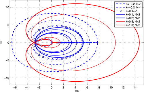
Figure 3 presents the stability loci about the k-related cases when $\beta =0.35$ and $\xi =-0.2$ are specified. Clearly, each and all the loci have one or two net encirclement(s) around the origin. Thus, in each case the closed-loop system is unstable by Theorem 4.1.

Figure 2. Complex scaling loci with $\beta =0.35$ and $\xi =0.2$.

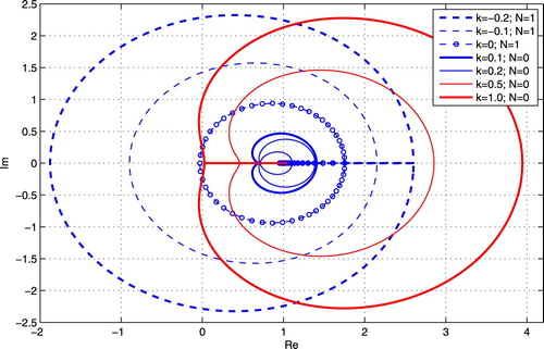
Figure 3. Complex scaling loci with $\beta =0.35$ and $\xi =-0.2$.

Indeed, the closed-loop state matrix of the example LCP system is $\begin{array}{rl}{A}_c\left(t\right)& =A\left(t\right)-B\left(t\right)kC\left(t\right)\\ & =\left[\begin{array}{cc}0& 1\\ -k(1-2\beta \cos {\omega }_{h}t)& -2\xi \end{array}\right]\end{array}$ Therefore, according to the Floquet theorem, asymptotical stability of the closed-loop LCP system can be tested by forming the so-called monodromy of $A_c\left(t\right)$, computing its eigenvalues and checking whether or not all eigenvalues are within the unit circle.

Figures 4 and 5 plot the monodromy eigenvalue loci of $A_c\left(t\right)$ under $k\in [-0.2,1]$ by the dotted lines with $\xi =0.2$ and $\xi =-0.2$, respectively, whereas $\beta =0.35$ is fixed. In these figures, the dashed-line curves illustrate the unit circle. Due to the inequitable scaling in the x- and y-axes, the unit circles turn out to be ovals in shape. The crosses, namely ×'s, denote the eigenvalues at k=−1, and the tiny circles, namely °'s, stand for those at k=1.

Figure 4. Monodromy eigenvalue loci of $A_c\left(t\right)$ for $k\in [-0.2,1]$ with $\beta =0.35$ and $\xi =0.2$.

Figure 5. Monodromy eigenvalue loci of $A_c\left(t\right)$ for $k\in [-0.2,1]$ with $\beta =0.35$ and $\xi =-0.2$.

Comparing Figure 4 (resp, Figure 5) to Figure 2 (resp., Figure 3), one can quickly find that the monodromy eigenvalue loci validate the stability assertions.

6.2. Stabilization illustration

Figure 3 says that when $\xi <0$, the lossy Mathieu equation cannot be stabilised via static output feedback, due to uncontrollability (Zhou et al., 2016). To address this problem, we additionally install a static state feedback $v\left(t\right)=-[0,1{]}^{T}K\zeta (t)$ with $K=[k_1,k_2]$, beside the static output feedback $u\left(t\right)=-ky\left(t\right)$, and the closed-loop system is described by $\dot{\zeta }\left(t\right)=\left[A\right(t)-[0,1{]}^{T}K-B\left(t\right)kC\left(t\right)\left]\zeta \right(t)$ Clearly, the closed-loop state matrix is still h-periodic. In the sequel, we illustrate that by pole assignment about the eigenvalues of $A_0-[0,1{]}^{T}K$, stabilisation of the closed-loop LCP system is attainable even if $\xi <0$.

The characteristic polynomial for $A_0-[0,1{]}^{T}K$ is $det(s{I}_n-A_0+[0,1{]}^{T}K)=s^2+(2\xi +k_2)s+k_1$ Then, the closed-loop eigenvalues are ${\lambda }_{1,2}=\frac{1}{2}[-(2\xi +k_2)\pm \sqrt{(2\xi +k_2{)}^2-4k_1}]$ Hence, by choosing $k_1$ and $k_2$ appropriately, the eigenvalues of $A_0-[0,1{]}^{T}K$ can be assigned arbitrarily. This is not surprising since $(A_0,[0,1{]}^T)$ is controllable.

In particular, if we let $k_1$ and $k_2$ satisfy $2\xi +k_2>0$ and $4k_1>(2\xi +k_2{)}^2$, then the eigenvalues of $A_0-[0,1{]}^{T}K$ can be a pair of complex conjugates with negative real parts. Moreover, if stability robustness is concerned, the bigger $k_2>0$ is, the better. For example, when $K=[3.40,3.25]$ that assigns the eigenvalues at $-1.4250\pm 1.1702j$, the complex scaling loci are given in Figure 6 as the output feedback gain varies over $k\in [-0.2,1.0]$. Clearly, in each k, the complex scaling locus neither passes through nor encircles the origin. Theorem 4.1 says that the closed-loop LCP system is stabilised. This can also be verified simply by Theorem 5.1 as well as Theorem 5.2.

The monodromy eigenvalue loci of the closed-loop LCP system are given in Figure 7. It must be pointed out that since the unit circle is far beyond the plotting range of Figure 7, the eigenvalue loci are entirely located within the unit circle. This coincides with the results of Figure 6.

As comparison with some existing stability analysis methods for LCP systems, stability analysis about the same lossy Mathieu differential equation were reported in Zhou et al. (2002) and Zhou and Hagiwara (2005), where Floquet factorisation and Fourier series are heavily relied upon and thus the numerical implementation is a hard task. What is more, stabilisation is hampered simply due to Floquet factorisation and harmonic analysis. In view of these facts, it is reasonable to say that the suggested approaches are promising in analysis and synthesis of LCP control systems.

Figure 6. Complex scaling loci of stabilisation under the feedback gain $K=[3.40,3.25]$ with $\beta =0.35$ and $\xi =-0.2$.

Figure 7. Monodromy eigenvalue loci of $A_c\left(t\right)$ for $k\in [-0.2,1]$ under $K=[3.40,3.25]$ with $\beta =0.35$ and $\xi =-0.2$.

7. Conclusions

In this study, we establish an alternative 2-regularised stability criterion for LCP systems by means of complex scaling. The main results are summarised in Theorem 3.1 in term of infinite-dimensional Toeplitz operators, which has a finite-dimensional version as in Theorem 4.1. These criteria make it possible to test asymptotic stability in feedback LCP systems through frequency-domain features without open-loop structural knowledge and Floquet factorizations. How to exploit these advantages for stabilisation in the LCP setting is also scrutinised in the paper. The main results are summarised in Theorems 5.1 and 5.2.

Technical significance of the study is that without Floquet-Lyapunov transformation, Nyquist-like criteria can still be developed in LCP feedback systems for stability analysis and stabilisation, even if no open-loop structural features are available. Such technical advantages do not exist if working with numerical monodromy computation. This is especially the case when the concerned LCP systems are high-dimensional and with multiple feedbacks.

Disclosure statement

No potential conflict of interest was reported by the author.

ORCID

J. Zhou  http://orcid.org/0000-0002-2907-7269

Additional information

Funding

This study was supported by the National Nature Science Foundation of China under Grant No. 61573001.

References

- Allievi, A., & Soudack, A. (1990). Ship stability via the Mathieu equation. International Journal of Control, 51, 139–167. doi: 10.1080/00207179008934054
- Bernstein, D. S. (2009). Matrix mathematics: Theory, facts and formulas (2nd ed.). New Jersey: Princeton University Press.
- Bittanti, S., & Colaneri, P. (2001). Stabilization of periodic systems: overview and advances. In Proceedings of IFAC Workshop on Periodic Control Systems (pp. 157–162), Italy.
- Bolzern, P., & Colaneri, P. (1988). The periodic Lyapunov equation. SIAM Journal of Matrix Analysis and Applications, 9, 499–512. doi: 10.1137/0609041
- Böttcher, A., & Silbermann, B. (1990). Analysis of Toeplitz operators. Berlin: Springer-Verlag.
- Cantoni, M., & Glover, K. (2000). Existence of right and left representations of the graph for linear periodically time-varying systems. SIAM Journal of Control and Optimization, 38, 786–802. doi: 10.1137/S0363012998346608
- Conway, J. B. (1990). A course in functional analysis (2nd ed.). New York: Springer.
- Dugundji, J., & Wendelll, J. H. (1983). Some analysis methods for rotating systems with periodic coefficients. AIAA Journal, 21, 890–897. doi: 10.2514/3.8167
- Farkas, M. (1994). Periodic motions. New York: Springer-Verlag.
- Gohberg, I., Goldberg, S., & Kaashoek, M. A. (1993). Classes of linear operators (Vol. II). Birlin: Birkhäuser.
- Gohberg, I., Goldberg, S., & Krupnik, N. (2000). Traces and determinants of linear operators. Berlin: Birkhäuser.
- Guckenheimer, J., & Holmes, P. (1983). Nonlinear oscillations, dynamical systems, and bifurcations of vector fields. New York: Springer-Verlag.
- Haddad, W. M., & Chellabonina, V. (2008). Nonlinear dynamical systems and control: A Lyapunov-based approach. Oxford: Princeton University Press.
- Halanay, A. (1966). Differential equations: Stability, oscillations, time lags. New York: Academic Press.
- Hall, S. R., & Wereley, N. W. (1990). Generalized criterion for linear time systems. In Proceedings of the 1990 American Control Conference (pp. 1518–1525), San Diego.
- Kao, C. Y., Megretski, A., & Jonsson, U. T. (2001). A cutting plane algorithm for robustness analysis of periodically time-varying systems. IEEE Transactions on Automatic Control, 46, 579–592. doi: 10.1109/9.917659
- Khalil, H. (2000). Nonlinear systems (3rd ed.). New Jersey: Pearson Educational International Inc.
- Lakshmikantham, V., Leela, S., & Martynyuk, A. A. (1989). Stability analysis of nonlinear systems. New York and Basel: Marchel Dekker, Inc.
- Lampe, B. P., & Rossenwasser, E. N. (2010). Using the Fredholm resolvent for computing the H2-norm of linear periodic systems. International Journal of Control, 83(9), 1868–1884. doi: 10.1080/00207179.2010.498060
- Lampe, B. P., & Rossenwasser, E. N. (2011). Stability investigation for linear periodic time-delayed sytems using Fredholm theory. Automation and Remote Control, 72(1), 38–60. doi: 10.1134/S0005117911010048
- Lukes, D. L. (1982). Differential equations: Classical to controlled. New York: Academic Press.
- Montagnier, P., Spiteri, R. J., & Angeles, J. (2004). The control of linear time-periodic systems using Floquet-Lyapunov theory. International Journal of Control, 77, 472–490. doi: 10.1080/00207170410001667477
- Nayfeh, A. H., & Mook, D. T. (1979). Nonlinear oscillations. New York: Wiley.
- Richards, J. A. (1983). Analysis of periodically time-varying system. New York: Springer-Verlag.
- Stein, E. M., & Shakarchi, R. (2003). Complex analysis. New Jersey: Princeton University Press.
- Yakubovich, V. A. (1988). Dichotomy and absolute stability of nonlinear systems with periodically non-stationary linear part. Systems & Control Letters, 11, 221–228. doi: 10.1016/0167-6911(88)90062-X
- Zhou, J. (2013). Contraposition 2-regularized Nyquist criterion in linear continuous-time periodic systems. In Proceedings of the 5th IFAC Workshop on Periodic Control Systems (pp. 149–154), Caen, France.
- Zhou, J. (2017). Complex-domain stability criteria for fractional-order linear dynamical systems. IET Control Theory and Applications, 11(16), 2753–2760. doi: 10.1049/iet-cta.2016.1578
- Zhou, J. (2018). Interpreting Popov criteria in Luré systems with complex scaling stability analysis. Communications in Nonlinear Science and Numericalal Simulation, 59, 306–318. doi: 10.1016/j.cnsns.2017.11.029
- Zhou, K. M., & Doyle, J. C. (1998). Essentials of Robust control. New York: Prentice Hall.
- Zhou, J., Gao, K. T., & Lu, X. B. (2018). Complex scaling approach for stability analysis and stabilization of multiple time-delayed systems. Mathematical Problems in Engineering, 2018, Article ID: 8492735, 14 pages.
- Zhou, J., Hagiwara, T., & Araki, M. (2002). Stability analysis of continuous-time periodic systems via the harmonic analysis. IEEE Transactions on Automatic Control, 47, 292–298. doi: 10.1109/9.983361
- Zhou, J., & Hagiwara, T. (2005). 2-regularized Nyquist criterion in linear continuous-time periodic systems and its implementation. SIAM Journal of Control and Optimization, 44, 618–645. doi: 10.1137/S0363012902416900
- Zhou, J., Lu, X. B., & Qian, H. M. (2016). Controllability discrepancy and irreducibility/reducibility of Floquet factorizations in linear continuous-time periodic systems. International Journal of Systems Science, 47, 2965–2974. doi: 10.1080/00207721.2015.1053830
- Zhou, J., & Qian, H. M. (2017a). Pointwise frequency responses framework for stability analysis in periodically time-varying systems. International Journal of Systems Science, 48, 715–728. doi: 10.1080/00207721.2016.1212430
- Zhou, J., & Qian, H. M. (2017b). Stability analysis of sampled-data systems via open/closed-loop characteristic polynomials contraposition. International Journal of Systems Science, 48(9), 1941–1953. doi: 10.1080/00207721.2017.1290298
- Zhou, J., Qian, H. M., & Lu, X. B. (2017). An argument-principle-based framework for structural and spectral characteristics in linear dynamical systems. International Journal of Control, 90(12), 2598–2604. doi: 10.1080/00207179.2016.1260163