
 ?Mathematical formulae have been encoded as MathML and are displayed in this HTML version using MathJax in order to improve their display. Uncheck the box to turn MathJax off. This feature requires Javascript. Click on a formula to zoom.
ABSTRACT
This study proposes an efficient Newton-type method for the optimal control of switched systems under a given mode sequence. A mesh-refinement-based approach is utilised to discretise continuous-time optimal control problems (OCPs) and formulate a nonlinear program (NLP), which guarantees the local convergence of a Newton-type method. A dedicated structure-exploiting algorithm (Riccati recursion) is proposed to perform a Newton-type method for the NLP efficiently because its sparsity structure is different from a standard OCP. The proposed method computes each Newton step with linear time-complexity for the total number of discretization grids as the standard Riccati recursion algorithm. Additionally, the computation is always successful if the solution is sufficiently close to a local minimum. Conversely, general quadratic programming (QP) solvers cannot accomplish this because the Hessian matrix is inherently indefinite. Moreover, a modification on the reduced Hessian matrix is proposed using the nature of the Riccati recursion algorithm as the dynamic programming for a QP subproblem to enhance the convergence. A numerical comparison is conducted with off-the-shelf NLP solvers, which demonstrates that the proposed method is up to two orders of magnitude faster. Whole-body optimal control of quadrupedal gaits is also demonstrated and shows that the proposed method can achieve the whole-body model predictive control (MPC) of robotic systems with rigid contacts.
1. Introduction
Switched systems are a class of hybrid systems consisting of a finite number of subsystems and switching laws of active subsystems. Many practical control systems are modeled as switched systems, such as real-world complicated process systems (Bürger et al., Citation2019), automotive systems with gear shifts (Robuschi et al., Citation2021), and robotic systems with rigid contacts (Farshidian et al., Citation2017; Li & Wensing, Citation2020). It is difficult to solve the optimal control problems (OCPs) of such systems because these OCPs generally involve mixed-integer nonlinear programs (MINLPs) (Belotti et al., Citation2013). Therefore, model predictive control (MPC) (Rawlings et al., Citation2017), in which OCPs must be solved in real-time, is particularly difficult for switched systems. One of the most practical approaches for solving the OCPs of switched systems is the combinatorial integral approximation (CIA) decomposition method (Bürger et al., Citation2019; Sager et al., Citation2011). CIA decomposition relaxes the MINLP into a nonlinear program (NLP) in which the binary variables are relaxed into continuous variables. Subsequently, the integer variables are approximately reconstructed from the relaxed NLP solution by solving a mixed-integer linear program. However, vanishing constraints, which typically model mode-dependent path constraints, raise numerical issues due to the violation of the linear independence constraint qualification (LICQ) (Jung et al., Citation2013). A similar smoothing approach is used for discrete natures when solving OCPs for mechanical systems with rigid contacts, which are often approximately formulated as mathematical programs with complementarity constraints (MPCCs) (Posa et al., Citation2014; Yunt, Citation2011). However, this case has the same LICQ problem as the vanishing constraints, requiring a significant amount of computational time to alleviate the numerical ill-conditioning. Furthermore, it often suffers from undesirable stationary points (Nurkanović et al., Citation2020).
Another tractable and practical approach for the optimal control of switched systems is to fix the switching (mode) sequence. For example, in robotics applications, a high-level planner computes the feasible contact sequence taking perception into account. Subsequently, the sequence is provided to a lower-level optimal control-based dynamic motion planner or MPC controller (Grandia et al., Citation2021; Jenelten et al., Citation2020; Kuindersma et al., Citation2016). The lower-level dynamic planner or MPC then discovers the optimal switching times and optimal control input. An advantage of this approach over the CIA decomposition and MPCC approaches is that the optimization problem is smooth and can, therefore, be efficiently solved without suffering from the LICQ problem. For example, Johnson and Murphey (Citation2011) and Stellato et al. (Citation2017) proposed efficient Newton-type methods for OCPs of switched systems with autonomous subsystems. That is, the switched systems only included a switching signal but no continuous control input, which is called the switching-time optimization (STO) problem. The STO approach can be more efficient than the CIA decomposition because the STO problem can be formulated as a smooth and tractable NLP, as numerically shown in Stellato et al. (Citation2017). However, once the switched system includes a continuous control input, the efficient methods of Johnson and Murphey (Citation2011) and Stellato et al. (Citation2017) cannot be applied. To the best of our knowledge, there is no efficient numerical method for OCPs of such systems. As a result, many real-world robotic applications are limited to focusing on dynamic motion planning with fixed switching instants (Di Carlo et al., Citation2018; Farshidian et al., Citation2017; Mastalli et al., Citation2020).
The two-stage approach has been studied for the OCPs of switched systems with continuous control input (Farshidian et al., Citation2017; Fu & Zhang, Citation2021; Li & Wensing, Citation2020; Xu & Antsaklis, Citation2002, Citation2004). A general two-stage approach was proposed in Xu and Antsaklis (Citation2002, Citation2004). In this approach, the optimization problem to determine the control input and switching instants was decomposed into an STO problem with a fixed control input (upper-level problem) and standard OCP that only determined the control input with fixed switching instants (lower-level problem). In this framework, off-the-shelf OCP solvers can be used for a lower-level problem. Xu and Antsaklis (Citation2004) formulated the lower-level continuous-time OCP as a two-point boundary-value problem and leveraged off-the-shelf shooting methods to solve it. Farshidian et al. (Citation2017), Li and Wensing (Citation2020), and Xu and Antsaklis (Citation2002) formulated the lower-level problem as an NLP by using the direct single shooting method and solved it using off-the-shelf Newton-type methods. However, these studies still lack convergence speed because each of these two stages does not take the other stage into account when solving its own optimization problem. As a result, the application examples of Farshidian et al. (Citation2017) and Li and Wensing (Citation2020) were limited to off-line computation for the trajectory optimization problems of simplified robot models. Moreover, they could not guarantee the local convergence or address inequality constraints. The study of Fu and Zhang (Citation2021) was the first study that guaranteed convergence with a finite number of iterations and treated inequality constraints within a two-stage framework. However, it still required extensive computational time until convergence, even for a considerably simple linear quadratic example.
Other approaches simultaneously optimise the switching instants and other variables, such as the state and control input (Betts, Citation2010; Katayama et al., Citation2020; Katayama & Ohtsuka, Citation2021c; Patterson & Rao, Citation2014). A multi-phase trajectory optimization (Betts, Citation2010; Patterson & Rao, Citation2014) naturally incorporated the STO problem into the direct transcription, solving the NLP to simultaneously determine all variables (including the state, control input, and switching instants) using general-purpose off-the-shelf NLP solvers, such as Ipopt (Wächter & Biegler, Citation2006). However, the computational speed of general-purpose linear solvers used in off-the-shelf NLPs can typically be further improved, particularly, for large-scale systems because they have a certain sparsity structure (Rao et al., Citation1998; Wang & Boyd, Citation2010; Zanelli et al., Citation2020). In Katayama et al. (Citation2020), we applied the simultaneous approach with the direct single-shooting method and achieved real-time MPC for a simple walking robot using the Newton–Krylov type method (Ohtsuka, Citation2004). In Katayama and Ohtsuka (Citation2021c), we formulated an NLP using the direct multiple-shooting method (Bock & Plitt, Citation1984) and proposed a Riccati recursion algorithm for the NLP, which achieved faster computational time compared with the two-stage methods. However, these methods lacked the convergence guarantee due to the irregular discretization of the continuous-time OCP, which changed the problem structure throughout the Newton-type iterations. As a result, the method from Katayama and Ohtsuka (Citation2021c) could only converge when the initial guess of the switching instants was close to the optimal one in the numerical example.
This study proposes an efficient Newton-type method for optimal control of switched systems under a given mode sequence. First, a mesh-refinement-based approach is proposed to discretise the continuous-time OCP using the direct multiple-shooting method (Bock & Plitt, Citation1984) to formulate an NLP that facilitates the local convergence of the Newton-type methods. Second, a dedicated efficient structure-exploiting algorithm (Riccati recursion algorithm Rao et al., Citation1998) is proposed for the Newton-type method because the sparsity structure of the NLP is different from the standard OCP. The proposed method computes each Newton step with linear time-complexity of the total number of the discretization grids as the standard Riccati recursion algorithm. Additionally, it can always solve the Karush–Kuhn–Tucker (KKT) systems arising in the Newton-type method if the solution is sufficiently close to a local minimum, so that the second-order sufficient condition (SOSC) holds. This is in contrast to some general quadratic programming (QP) solvers that cannot treat the proposed formulation because the Hessian matrix is inherently indefinite. Third, a modification on the reduced Hessian matrix is proposed to enhance the convergence using the nature of the Riccati recursion algorithm as the dynamic programming (Bertsekas, Citation2005) for a QP subproblem. Two numerical experiments were conducted to demonstrate the efficiency of the proposed method: a comparison with off-the-shelf NLP solvers and testing the whole-body optimal control of quadrupedal gaits. The comparison with off-the-shelf NLP solvers showed that the proposed method could solve the OCPs that the sequential quadratic programming (SQP) method with qpOASES (Ferreau et al., Citation2014) or OSQP (Stellato et al., Citation2020) failed to solve and was up to two orders of magnitude faster than a general NLP solver, Ipopt (Wächter & Biegler, Citation2006). The whole-body optimal control of quadrupedal gaits showed that the proposed method achieved the whole-body MPC of robotic systems with rigid contacts.
The remainder of this paper is organised as follows. A mesh-refinement-based discretization method of the continuous-time OCP is presented in Section 2. The KKT system to be solved to compute the Newton-step is discussed in Section 3, and the Riccati recursion algorithm to solve the KKT system and its convergence properties are described in Section 4. The reduced Hessian modification using the Riccati recursion algorithm is also described in this section. The above formulations and Riccati recursion algorithm are extended to switched systems with state jumps and switching conditions in Section 5, representing robotic systems with contacts. A numerical comparison of the proposed method with off-the-shelf NLP solvers and examples of whole-body optimal control of a quadrupedal robot are presented in Section 6. Finally, a brief summary and mention of future work are presented in Section 7.
Notation and preliminaries: The Jacobians and Hessians of a differentiable function using certain vectors are described as follows: denotes
, and
denotes
. A diagonal matrix whose elements are a vector x is denoted as
. A vector of an appropriate size with all components presented by
is denoted as
. All functions are assumed to be twice-differentiable.
2. Problem formulation
We consider a switched system consisting of K + 1 () subsystems, which is expressed as
(1)
(1) The system is subject to the following constraints:
(2)
(2) where
denotes the state,
denotes the control input,
, and
.
denotes the indices of the active subsystems. Note that the index k is also referred to as a ‘phase’ in this study.
and
denote the fixed initial and terminal times of the horizon, respectively.
,
denotes the switching instant from phase k to phase k + 1. We assume that the active subsystems switch in order from 1 to K + 1 over the horizon
, that is,
. We further assume that each subsystem
has to be active, at least for a given time duration
, called the minimum dwell-time. The OCP of the switched system for a given initial state
is expressed as
(3a)
(3a)
(3b)
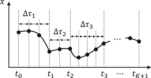
(3b) Next, a discretization method and mesh-refinement-based solution approach are proposed for the OCP to guarantee the local convergence. Figure illustrates the proposed discretization method. The OCP is discretised using the direct multiple-shooting method (Bock & Plitt, Citation1984) based on the forward Euler method so that all the time-steps in phase
are equal. Note that it is easy to extend the proposed method for higher-order explicit integration schemes to the direct multiple-shooting method, such as the fourth-order explicit Runge–Kutta method, as long as the Riccati recursion algorithm can be applied to the integration schemes. We introduce N grid points over the horizon, the discretised state
, discretised control input
, and switching instants
. The NLP is then expressed as
(4a)
(4a)
(4b)
(4b)
(4c)
(4c)
(4d)
(4d)
(4e)
(4e) Here,
is the set of stage indices at phase k (that is, the set of time stages where the subsystem equation
is active). Note that the last stage N is not included in any
. That is,
,
for
, and
hold for
.
is the time step at phase k, defined as
(4f)
(4f) where
is the number of grids in phase k, that is,
. Finally, the initial state condition is lifted as (Equation4b
(4b)
(4b) ), possibly for a real-time MPC implementation (Diehl et al., Citation2005).
Figure 1. Proposed discretization method for the OCPs of switched systems.
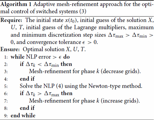
The continuous-time OCP (Equation3(3a)
(3a) ) is solved using an adaptive mesh-refinement approach (Betts, Citation2010), which consists of a solution of the NLP (Equation4
(4a)
(4a) ) using a Newton-type method and mesh-refinement due to the changes of
, as shown in Algorithm 1. After solving the NLP, the size of the discretization steps
is checked for each
. If the step is too large, that is, if it exceeds the specified threshold
, the solution at phase k may be not accurate. Therefore, the number of grids for phase k is increased. Conversely, if the step is too small (
), the number of grids for phase k is reduced to decrease the computational time of the next NLP step. The algorithm terminates if some criteria (for example,
norm of the KKT residual), which is denoted as ‘NLP error’ in Algorithm 1, is smaller than a predefined threshold
and the discretization steps pass the checks. By appropriately choosing
, the NLP dimension is almost constant throughout Algorithm 1. This is an advantage of the proposed method over direct transcription methods, such as Patterson and Rao (Citation2014), whose NLP dimension is unknown before being solved.
It is worth noting that the NLP (Equation4(4a)
(4a) ) is smooth and its structure does not change within each NLP step. Therefore, the Newton-type method for the NLP (Equation4
(4a)
(4a) ) is always tractable.
Remark 2.1
It is trivial to show the local (superlinear) convergence of Newton-type methods for the NLP (Equation4(4a)
(4a) ) under some reasonable assumptions (Nocedal & Wright, Citation2006). Moreover, if the solution guess after the mesh-refinement of Algorithm 1 is sufficiently close to a local minimum of the NLP after the mesh-refinement (that is, the mesh-refinement is sufficiently accurate), then the local convergence of the overall Algorithm 1 is also guaranteed. In contrast, previous methods cannot guarantee the local convergence, such as the two-stage approaches (Farshidian et al., Citation2017; Li & Wensing, Citation2020; Xu & Antsaklis, Citation2002, Citation2004) and simultaneous approaches with the other discretization methods (Katayama et al., Citation2020; Katayama & Ohtsuka, Citation2021c).
Note that it is assumed throughout this study that the state Equation (Equation1(1)
(1) ), inequality constraints (Equation2
(2)
(2) ), and cost function (Equation3a
(3a)
(3a) ) do not depend on the time. That is, they are time invariant for notational simplicity. However, it is possible to extend the proposed method to time-varying cases, where the time of each grid i that depends on the duration of phases
in (Equation1
(1)
(1) ), (Equation2
(2)
(2) ), and (Equation3a
(3a)
(3a) ) must be taken into account. Then, additional sensitivities of (Equation1
(1)
(1) ), (Equation2
(2)
(2) ), and (Equation3a
(3a)
(3a) ) with respect to the switching times are introduced in the KKT conditions and systems, which are derived in the next section. The formulations and methods of this study can be directly applied to such cases as long as the structure of the KKT system has the same form as the next section.
3. KKT system for Newton-type method
Next, the KKT system is derived to compute the Newton step of the NLP (Equation4(4a)
(4a) ). The inequality constraints are treated with the primal–dual interior point method (Nocedal & Wright, Citation2006; Wächter & Biegler, Citation2006). That is, the slack variables
and
are introduced for (Equation4d
(4d)
(4d) ) and (Equation4e
(4e)
(4e) ), respectively. The equality constraints are then considered, which are expressed as
(5a)
(5a)
(5b)
(5b) instead of the inequality constraints (Equation4d
(4d)
(4d) ) and (Equation4e
(4e)
(4e) ). The barrier functions
are also added to the cost function (Equation4a
(4a)
(4a) ), where
is the barrier parameter. An NLP associated with the barrier parameter ϵ is then expressed as
(6a)
(6a)
(6b)
(6b) where
and
.
We then derive the KKT conditions for the NLP (Equation6(6a)
(6a) ). To this end,
are introduced as the Lagrange multipliers with respect to (Equation4b
(4b)
(4b) ) and (Equation4c
(4c)
(4c) );
are with respect to (Equation5a
(5a)
(5a) ), and
are with respect to (Equation5b
(5b)
(5b) ). The Lagrangian of the NLP (Equation6
(6a)
(6a) ) is then given by
(7)
(7) where
(8)
(8) is the Hamiltonian at phase
. The KKT conditions of the NLP (Equation6a
(6a)
(6a) ) are then composed by the equality constraints (Equation4b
(4b)
(4b) ), (Equation4c
(4c)
(4c) ), (Equation5a
(5a)
(5a) ), and (Equation5b
(5b)
(5b) ) and the first-order derivatives of the Lagrangian (Equation7
(7)
(7) ) with respect to X, U, T, Z, and W, which are expressed as
(9a)
(9a)
(9b)
(9b)
(9c)
(9c)
(9d)
(9d)
(9e)
(9e) and
(9f)
(9f) We refer to the above KKT conditions as the perturbed KKT conditions in the following because the complementary slackness regarding the inequality constraints are perturbed with ϵ as (Equation9d
(9d)
(9d) ) and (Equation9e
(9e)
(9e) ) (Nocedal & Wright, Citation2006). Next, the KKT system is derived to compute the Newton steps of all variables, that is,
,
, and
. Note that the KKT system is herein considered as the standard primal–dual interior point method (Nocedal & Wright, Citation2006; Wächter & Biegler, Citation2006), in which the Newton steps regarding the inequality constraints are eliminated (that is,
and
). The KKT system of interest is then expressed as (note that
)
(10a)
(10a)
(10b)
(10b)
(10c)
(10c)
(10d)
(10d)
(10e)
(10e) and
(10f)
(10f) where
and
In addition,
is residual in (Equation4c
(4c)
(4c) ). Note that some of the phase index k is omitted from the KKT system Equation (Equation10
(10a)
(10a) ) because the phase index k is determined from i, and the matrices and vectors (other than the Newton steps in (Equation10
(10a)
(10a) )) are fixed once they are computed and therefore do not depend on the phase index k to solve the KKT system. The equations of the KKT system (Equation10a
(10a)
(10a) )–(Equation10f
(10f)
(10f) ) correspond to the KKT conditions (Equation4b
(4b)
(4b) ), (Equation4c
(4c)
(4c) ), (Equation9a
(9a)
(9a) )–(Equation9c
(9c)
(9c) ), and (Equation9f
(9f)
(9f) ), respectively.
Note that the KKT system (Equation10(10a)
(10a) ) is equivalent to the KKT conditions of a QP subproblem
(11)
(11) which is a quadratic approximation of the NLP (Equation4
(4a)
(4a) ). Subsequently,
can be regarded as the Lagrange multipliers of the QP with respect to (Equation10a
(10a)
(10a) ) and (Equation10b
(10b)
(10b) ) (Nocedal & Wright, Citation2006).
Remark 3.1
The Hessian matrix of (Equation11(11)
(11) ) is inherently indefinite, which makes solving the KKT system (Equation10
(10a)
(10a) ) difficult when using off-the-shelf QP solvers because they typically require a positive definite Hessian matrix. This can be explained with a block diagonal of the Hessian matrix (Equation11
(11)
(11) ), expressed as
(12)
(12) This is indefinite due to the off-diagonal terms
and
, even when:
.
4. Riccati recursion to solve KKT systems
In this section, a Riccati recursion algorithm is presented to compute the Newton step of the NLP (Equation4(4a)
(4a) ) by solving the KKT system (Equation10
(10a)
(10a) ). The sparsity structure of the KKT system (Equation10
(10a)
(10a) ) is no longer the same as the standard OCP, which prevents applying the off-the-shelf efficient Newton-type algorithms for OCPs (Rao et al., Citation1998; Wang & Boyd, Citation2010; Zanelli et al., Citation2020). Moreover, as stated in Remark 3.1, the Hessian matrix of the KKT system is indefinite and unsolvable using general QP solvers. Motivated by these problems, we propose a Riccati recursion algorithm that efficiently solves the KKT system, specifically with
computational time, whenever the SOSC holds. Moreover, a reduced Hessian modification method is proposed to enhance the convergence when the SOSC does not hold, that is, when the reduced Hessian matrix is indefinite. As the standard Riccati recursion (Rao et al., Citation1998), the proposed method is composed of backward and forward recursions, which recursively eliminate the variables from the KKT system (Equation10
(10a)
(10a) ) backward in time and recursively compute the Newton step forward in time, respectively.
4.1. Backward recursion
In the backward recursion, the Newton steps are recursively eliminated from stages N to 0. Specifically, expressions of ,
, and
are derived at each stage
for
,
, and
, respectively, from (Equation10b
(10b)
(10b) )–(Equation10e
(10e)
(10e) ). Moreover, variables are recursively eliminated from (Equation10f
(10f)
(10f) ) using these expressions. When the stage of interest changes from k to k−1,
is further eliminated from (Equation10f
(10f)
(10f) ). That is, an expression of
is derived with respect to
and
, where
. This can be seen as the extension of the standard Riccati recursion that also recursively derives expressions of
,
, and
with respect to
(Rao et al., Citation1998; Rawlings et al., Citation2017).
4.1.1. Terminal stage
From (Equation10c(10c)
(10c) ) at stage N, we obtain:
(13a)
(13a) where
(13b)
(13b)
4.1.2. Intermediate stages
Consider ,
. Suppose that we have the expression of
with respect to
,
, and
as
(14a)
(14a) where
and
. Furthermore, suppose that we have Equation (Equation10f
(10f)
(10f) ) for k and k−1 in which
for
,
for
, and
for
are eliminated, that is, Equation (Equation10f
(10f)
(10f) ) for k and k−1 are reduced to
(14b)
(14b) and
(14c)
(14c) where
. Note that
,
,
,
,
,
, and
at stage
. Moreover,
,
,
, and
at stages
and
, as explained in 4.1.3. First, the following equations are introduced:
(15a)
(15a)
(15b)
(15b)
(15c)
(15c)
(15d)
(15d)
(15e)
(15e) and
(15f)
(15f) Second,
and
are eliminated from (Equation10e
(10e)
(10e) ) using (Equation14a
(14a)
(14a) ) and (Equation10b
(10b)
(10b) ). Subsequently, we can express
using
,
, and
as
(16a)
(16a) where
(16b)
(16b)
(16c)
(16c) and
(16d)
(16d) Third,
,
, and
are eliminated from (Equation10d
(10d)
(10d) ) using (Equation14a
(14a)
(14a) ), (Equation10b
(10b)
(10b) ), and (Equation16a
(16a)
(16a) ), respectively. As a result,
using
,
, and
is expressed as
(17a)
(17a) where
(17b)
(17b)
(17c)
(17c) and
(17d)
(17d) Moreover, by eliminating
,
, and
from (Equation14b
(14b)
(14b) ) and (Equation14c
(14c)
(14c) ) using (Equation14a
(14a)
(14a) ), (Equation10b
(10b)
(10b) ), and (Equation16a
(16a)
(16a) ), we obtain:
(18a)
(18a) and
(18b)
(18b) where
(19a)
(19a)
(19b)
(19b)
(19c)
(19c)
(19d)
(19d) and
(19e)
(19e) Therefore, we have Equations (Equation17a
(17a)
(17a) ), (Equation18a
(18a)
(18a) ), and (Equation18b
(18b)
(18b) ) for stage i having the same form as that of Equation (Equation14
(14a)
(14a) ) for stage i + 1.
4.1.3. Phase transition stages
Here, we consider phase and stage
. In this stage, the phase of interest changes from k to k−1 when
, and the backward recursion terminates when k = 1. Equation (Equation14
(14a)
(14a) ) until
are expressed as
(20a)
(20a)
(20b)
(20b) and
(20c)
(20c) Note that
when k = 1. Therefore, from (Equation20b
(20b)
(20b) ),
is determined as
(21)
(21) Here, the following is defined:
(22)
(22) The backward recursion is completed when k = 1 because
. When k>1, (Equation21
(21)
(21) ) is further substituted into (Equation20a
(20a)
(20a) ) and (Equation20c
(20c)
(20c) ), which produces:
(23a)
(23a) and
(23b)
(23b) where
(23c)
(23c)
(23d)
(23d)
(23e)
(23e)
(23f)
(23f) and
(23g)
(23g) Therefore, we obtain Equations (Equation17a
(17a)
(17a) ), (Equation18a
(18a)
(18a) ), and (Equation18b
(18b)
(18b) ) for stage
in the same form as Equation (Equation14
(14a)
(14a) ) for stage i + 1 with
,
,
,
,
,
,
,
, and
.
4.2. Forward recursion
After the backward recursion up to the initial stage (i = 0), all Newton steps are recursively computed from stage 0 to N forward in time using the results of the backward recursion. First, the Newton step of the initial state is computed from (Equation10a
(10a)
(10a) ). Second, the Newton step of the first switching time
is computed from (Equation21
(21)
(21) ) with
. Third,
,
, and
are computed forward in time in each phase k using (Equation14a
(14a)
(14a) ), (Equation16a
(16a)
(16a) ), and (Equation10b
(10b)
(10b) ), respectively. Fourth, after this procedure,
is computed using (Equation21
(21)
(21) ) until stage
. The third and fourth steps are repeated from phase k = 1 to k = K + 1, and the forward recursion is completed by computing
using (Equation13a
(13a)
(13a) ).
The following lemma states the equivalence of the dynamic programming and the proposed Riccati recursion:
Lemma 4.1
Consider a phase and stage
. Suppose that
for all
, and
for all l>k, where
and
are defined in (Equation15c
(15c)
(15c) ) and (Equation22
(22)
(22) ), respectively. Then, the cost-to-go function of stage i of dynamic programming for the QP (Equation11
(11)
(11) ) is expressed as
(24)
(24) where
,
,
,
,
,
,
, and
are defined by the Riccati recursion algorithm presented in subsection 4.1. Moreover, the subproblem of the dynamic programming to determine
is represented by
(25)
(25) and determining
is expressed as
(26)
(26)
Proof.
The proof is achieved by induction. At the terminal stage (i = N), the cost-to-go function is represented by (Equation24(24)
(24) ) with
and
. Next, suppose that we have the cost-to-go function (Equation24
(24)
(24) ) of stage i + 1. Then, it is clear that the subproblem of the dynamic programming is represented by (Equation25
(25)
(25) ).
can be uniquely determined from (Equation25
(25)
(25) ) as (Equation16
(16a)
(16a) ) because
. The cost-to-go function of stage i is represented by (Equation24
(24)
(24) ), where
,
,
,
,
,
,
,
, and
are defined as (Equation15
(15a)
(15a) ), (Equation16
(16a)
(16a) ), (Equation17
(17a)
(17a) ), and (Equation19
(19a)
(19a) ). When
,
can be further uniquely determined by solving (Equation26
(26)
(26) ) under the assumption
after determining
and obtaining the cost-to-go function of stage
(Equation24
(24)
(24) ). Then, the cost-to-go function of stage
is in the form of (Equation24
(24)
(24) ), where
,
,
,
, and
are defined as (Equation23
(23a)
(23a) ),
,
,
, and
, respectively, which completes the proof.
Note that the equivalence cannot be shown without the positive definiteness of and
: if they are not positive definite, a unique solution does not exist and the cost-to-go function is not defined. The following theorem is obtained based on Lemma 4.1. Note that the discussion herein is restricted to the exact Hessian matrix to analyze the SOSC.
Theorem 4.2
We suppose that the SOSC and LICQ hold at the current iterate and consider that the exact Hessian matrix is used. Then, , as defined in (Equation15c
(15c)
(15c) ), is positive definite for all
. Moreover,
, as defined in (Equation22
(22)
(22) ), satisfies
for all
.
Proof.
The QP subproblem (Equation11(11)
(11) ) with an exact Hessian matrix must have a unique global solution because the SOSC and LICQ hold (Nocedal & Wright, Citation2006). Therefore, the dynamic programming subproblems (Equation25
(25)
(25) ) and (Equation26
(26)
(26) ) must have unique solutions. Subsequently, the Hessian matrix with respect to
in (Equation25
(25)
(25) ) must be positive definite, and the quadratic term with respect to
in (Equation26
(26)
(26) ) must be positive. Then, Lemma 4.1 recursively shows that the Hessian matrix is
with respect to
. Additionally, the lemma also shows that the quadratic term with respect to
is
, which completes the proof.
Theorem 4.2 indicates that can always be efficiently computed using Cholesky factorizations if the current iterate is sufficiently close to a local minimum. This fact also leads to the local (superlinear) convergence of the proposed method for NLP (Equation4
(4a)
(4a) ) under the SOSC and LICQ. The proof for this is omitted because it is trivial.
4.3. Reduced Hessian modification via Riccati recursion
The recused Hessian matrix can be indefinite when the solution is not sufficiently close to a local minimum, such that the SOSC does not hold. Subsequently, the KKT matrix is no longer invertible and the local convergence is not guaranteed. Efficient Cholesky factorization cannot be used to compute . Therefore, an algorithmic modification of the Riccati recursion is proposed to make the algorithm numerically robust and efficient for such situations, which can be considered a modification on the reduced Hessian matrix. To consider practical situations, Hessian approximations are allowed in the following, while Theorem 4.2 analyzes the exact Hessian matrix. First, we introduce the following practical assumption:
Assumption 4.1
and
for all
,
for all
, and
.
This assumption is easily satisfied with the Gauss-Newton Hessian approximation or, more generally, with sequential convex programming (Messerer et al., Citation2021) for ,
, and
. Under Assumption 4.1, a unique solution of the dynamic programming subproblem (Equation25
(25)
(25) ) exists (that is,
) and
if
, which is the same discussion as the dynamic programming for standard linear quadratic OCPs (Bertsekas, Citation2005). The solution to (Equation26
(26)
(26) ) also exists if
. Based on these observations, a modification of the Riccati recursion algorithm is proposed, whereby
is updated at each phase-transition stage
. This is expressed as
(27)
(27) instead of (Equation23c
(23c)
(23c) ). Then,
, as long as
. Note that a different method of (Equation27
(27)
(27) ) can be used to make
, which eliminates the negative curvature from
through eigenvalue decomposition (Quirynen et al., Citation2014). However, this requires considerably more computational time than (Equation27
(27)
(27) ). Nevertheless, the computationally cheap modification (Equation27
(27)
(27) ) works surprisingly well in practise. We also modify
instead of (Equation22
(22)
(22) ), which is expressed as
(28)
(28) where
and
. A practical rule to choose
and
is as follows. We empirically observed that numerical ill-conditioning in the Newton-type method produced a large
, that is, a too small
in (Equation21
(21)
(21) ). From this observation, a desired maximum absolute value of
was chosen as
. Subsequently,
and
were chosen such that the absolute value of
did not exceed
. This is expressed as
(29)
(29) for each
. For example, it was discovered that choosing
from a range of 0.1 to 1.0 worked well in practise.
The following Theorem claims that the proposed algorithmic modification makes the reduced Hessian matrix of the KKT system (Equation10(10a)
(10a) ) positive definite and the KKT matrix invertible:
Theorem 4.3
Suppose that Assumption 4.1 holds. Then, the reduced Hessian matrix of the KKT system (Equation10a(10a)
(10a) ) with the modifications (Equation27
(27)
(27) ) and (Equation28
(28)
(28) ) is positive definite. If, in addition, the LICQ holds, then the KKT matrix is invertible.
Proof.
Under Assumption 4.1 and with the Hessian modifications (Equation27(27)
(27) ) and (Equation28
(28)
(28) ),
for all
,
for all
, and
for all
hold. Therefore, the QP subproblems of the dynamic programming (Equation25
(25)
(25) ) and (Equation26
(26)
(26) ) always have unique global solutions. Theorem 16.2 of Nocedal and Wright (Citation2006) completes the first claim. The second claim then directly follows from Theorem 16.1 of Nocedal and Wright (Citation2006).
Remark 4.1
The KKT matrix is always invertible under Assumption 4.1 and the proposed reduced Hessian modifications. Therefore, the local convergence of the Newton-type method is ensured if the resultant reduced Hessian is sufficiently close to the exact one (Messerer et al., Citation2021; Nocedal & Wright, Citation2006) and the LICQ holds.
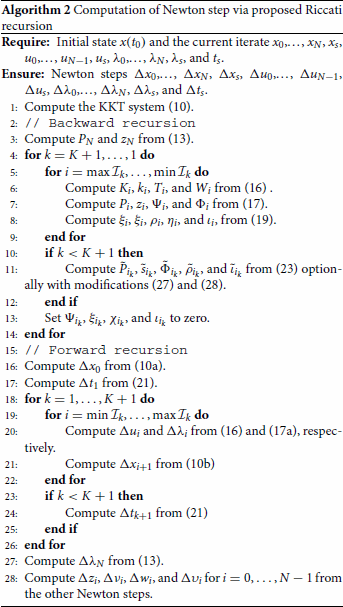
4.4. Summary of algorithm
The single Newton iteration using the proposed Riccati recursion algorithm is summarised in Algorithm 2. After computing the KKT system (Equation10(10a)
(10a) ) (line 1), the proposed method recursively eliminates the Newton steps from the KKT system (Equation10
(10a)
(10a) ) in the backward recursion (lines 3–14) and recursively computes the Newton steps in the forward recursion (lines 16–27). Finally, the Newton steps of the slack variables and Lagrange multipliers are computed from the other Newton steps (line 28) according to the primal–dual interior point method (Nocedal & Wright, Citation2006; Wächter & Biegler, Citation2006). Calculations in the proposed algorithm, such as matrix inversions or matrix–matrix multiplications, do not grow with respect to the length of the horizon N. Therefore, the computational time of the proposed method is
as the standard Riccati recursion algorithm (Rao et al., Citation1998). After computing the Newton steps, we can employ typical line-search methods, such as the merit function-based methods or filter-based methods (Nocedal & Wright, Citation2006), for the smooth constrained NLP (Equation6
(6a)
(6a) ).
5. State jumps and switching conditions
In this section, the proposed NLP formulations and Riccati recursion algorithm are further extended to switched systems involving state jumps and switching conditions, which have not yet been considered. Some classes of switched systems involve state jumps at the same time as the switch, which is expressed as
(30)
(30) where
is the instant immediately before
. We also consider that there is a stage cost on the state immediately before the state jump. That is, it is assumed that
is added to the cost function (Equation3a
(3a)
(3a) ). Moreover, such switches are often state-dependent, that is, the switch occurs if the state satisfies some condition (hereafter called the switching condition), which is expressed as
(31)
(31) For example, a legged robot can be modeled as a system with switches involving state jumps and switching conditions. When the distance between the robot's foot and the ground becomes zero (the switching condition), the generalised velocity instantly changes due to the impact (the state jump) (Farshidian et al., Citation2017; Li & Wensing, Citation2020).
If there is a state jump at the kth switch, a new grid point is introduced corresponding to time
, which is added to the KKT conditions and expressed as
(32a)
(32a) and
(32b)
(32b) The KKT systems regarding the state jump are therefore expressed as
(33a)
(33a) and
(33b)
(33b) where
and
is the Hessian of the Lagrangian with respect to
.
and
are the residuals in (Equation32a
(32a)
(32a) ) and (Equation32b
(32b)
(32b) ), respectively. When (Equation33a
(33a)
(33a) ) and (Equation33b
(33b)
(33b) ) are considered in the backward recursion, we have the equations until stage
. That is, the equations are in the form of (Equation23a
(23a)
(23a) ), (Equation23b
(23b)
(23b) ), and (Equation10f
(10f)
(10f) ), with the phase index k replaced with k−1. By eliminating
and
from these equations using (Equation33a
(33a)
(33a) ) and (Equation33b
(33b)
(33b) ), we then obtain
(34a)
(34a)
(34b)
(34b) and
(34c)
(34c) where
(34d)
(34d)
(34e)
(34e)
(34f)
(34f) and
(34g)
(34g) Therefore, the same equation as (Equation17
(17a)
(17a) ) is achieved at stage
, and we can proceed to stage
. In the forward recursion,
is computed from
and
using (Equation10b
(10b)
(10b) ) at stage
. Then,
and
are computed from
according to (Equation33a
(33a)
(33a) ) and (Equation17a
(17a)
(17a) ) for
with
.
5.1. Switching conditions
The switching conditions are typically presented as pure-state equality constraints, which are difficult to treat efficiently with the Riccati recursion algorithm (specifically with the computational burden) (Sideris & Rodriguez, Citation2011). In this section, we assume that the state is partitioned into the generalised coordinate and velocity as
,
and the state equation of each subsystem is expressed as
(35)
(35) where
and
. Moreover, we assume that the pure-state equality constraints representing the switching conditions have a relative degree of two, that is, the Jacobian of (Equation31
(31)
(31) ) is expressed as
(36)
(36) These assumptions mainly represent the position-level constraints on mechanical systems, such as robotic systems having rigid contacts. To use the Newton-type method with
complexity under these assumptions, we did not consider the pure-state equality constraint
(37)
(37) directly as was considered by Sideris and Rodriguez (Citation2011). Instead, the constraint was transformed into a mixed state-input constraint at the two-stage grid point before the switch (Katayama & Ohtsuka, Citation2021a), which is expressed as
(38)
(38) where i is two-stage before the grid
, that is, i satisfies
. The Lagrange multiplier is introduced with respect to (Equation38
(38)
(38) ),
. The KKT conditions regarding this stage are then represented by (Equation4c
(4c)
(4c) ), (Equation38
(38)
(38) ),
, and
, where
and
. Furthermore, the KKT conditions of (Equation9f
(9f)
(9f) ) related to
are replaced with:
and
where
. The KKT systems regarding this stage are then expressed as (Equation10b
(10b)
(10b) ),
(39a)
(39a)
(39b)
(39b) and
(39c)
(39c) where
and
In addition,
is residual in (Equation38
(38)
(38) ).
In the backward recursion at stage i, we have (Equation14a(14a)
(14a) ),
(40a)
(40a) and
(40b)
(40b)
and
are then eliminated, resulting in:
(41a)
(41a) where
(41b)
(41b)
(41c)
(41c)
(41d)
(41d) and
(41e)
(41e) Therefore, we obtain the form equations of (Equation17a
(17a)
(17a) ), (Equation18a
(18a)
(18a) ), and (Equation18b
(18b)
(18b) ) for stage i with the following:
(42a)
(42a)
(42b)
(42b) and
(42c)
(42c)
(43a)
(43a)
(43b)
(43b)
(43c)
(43c)
(43d)
(43d) and
(43e)
(43e) At the forward recursion,
and
are computed using (Equation41a
(41a)
(41a) ) instead of only computing
as (Equation16a
(16a)
(16a) ).
5.2. Summary of algorithm
We herein summarise the proposed algorithm for the OCPs with state jumps and switching conditions as an extension of Algorithm 2. The overall algorithm is the same as Algorithm 2 except for the computations around and
for
The computation of the KKT system (line 1 of Algorithm 2) now includes the computation regarding state jumps such as (Equation33a
(33a)
(33a) ) and (Equation33b
(33b)
(33b) ) when
and these regarding switching conditions such as (Equation39a
(39a)
(39a) )–(Equation39c
(39c)
(39c) ) when
for
. In the backward recursion (lines 3–14 of Algorithm 2), we compute the terms such as
and
using (Equation34d
(34d)
(34d) )–(Equation34g
(34g)
(34g) ) when
and (Equation42a
(42a)
(42a) )–(Equation43e
(43e)
(43e) ) when
for
. In the forward recursion (lines 16–27 of Algorithm 2), we additionally utilise (Equation33a
(33a)
(33a) ) and (Equation33b
(33b)
(33b) ) to compute
and
when
and (Equation41a
(41a)
(41a) ) to compute
and
when
for
.
6. Numerical experiments
6.1. Comparison with off-the-shelf solvers
6.1.1. Problem settings
The effectiveness of the proposed method was demonstrated through two numerical experiments. The first experiment was a comparison with off-the-shelf NLP solvers on the switched system, consisting of three nonlinear subsystems treated in Xu and Antsaklis (Citation2002, Citation2004). The dynamics of the subsystems are expressed as
and
The stage cost is expressed as
In addition, the terminal cost is expressed as
where
. The initial and terminal times of the horizon are denoted by
and
, respectively. The initial state is denoted by
.
Benchmarks were set for the solution times of the NLP (Equation4(4a)
(4a) ) example against the Ipopt (Wächter & Biegler, Citation2006) and a SQP methods with qpOASES (Ferreau et al., Citation2014), both of which were used through the CasADi (Andersson et al., Citation2019) interface. The mesh-refinement was not considered in this comparison to focus on a pure comparison of the abilities to solve the NLP problems. That is, only the single NLP step of Algorithm 1 was considered. Ipopt was used with the default settings of CasADi. For example, MUMPS (Amestoy et al., Citation2001) was used to solve the linear systems. The built-in SQP solver of CasADi was used with the exact Hessian matrix and qpOASES as the backend QP solver. The Hessian regularization was enabled within the qpOASES options and the Hessian type was set to ‘indefinite’. The proposed method was written in C++, used Eigen (Guennebaud & Jacob, Citation2010) for the linear algebra, and used an exact Hessian matrix and reduced Hessian modifications (Equation27
(27)
(27) ) and (Equation28
(28)
(28) ) throughout the experiments.
and
were chosen using (Equation29
(29)
(29) ) with
. The proposed method only used the fraction-to-boundary rule (Nocedal & Wright, Citation2006; Wächter & Biegler, Citation2006) for the step size selection and monotonically decreased the barrier parameter ϵ when the
norm of the KKT residual (in the perturbed KKT conditions (Equation9
(9a)
(9a) )) was smaller than 0.1. The solution times were compared for these algorithms with the total number of grids set as N = 10, 50, 100, and 500. N was divided into
,
, and
, so that each phase had an almost equal number of discretization grids. The values of
were set to
,
,
, and
for N = 10, 50, 100, and 500, respectively. The minimum dwell-times were set as
in the constraints (Equation4e
(4e)
(4e) ) to avoid ill-conditioned problems. The initial guess of the solution was set as
,
,
, and
for all solvers. It was assumed that the proposed method converged when the solution satisfied the default convergence criteria of Ipopt (max norm of the residual in the unperturbed KKT conditions (Nocedal & Wright, Citation2006; Wächter & Biegler, Citation2006)). All solvers were run 100 times for each N on a laptop with a quad-core CPU Intel Core i7-10510U @1.80 GHz, and the average computational time until convergence was measured.
6.1.2. Results
The average computational times of each solver for the different total number of grids N are listed in Table . As shown in the table, the proposed method converged the fastest of all the cases, and was up to two orders of magnitude faster than Ipopt. The proposed method was extremely fast because the dimension of the control input of each subsystem was 1 and it did not involve any explicit matrix inversions. The SQP method with qpOASES failed to converge for all cases, even the regularization and indefinite-Hessian mode were enabled. Note that another QP solver OSQP (Stellato et al., Citation2020) was also tested, but it failed to treat the indefinite Hessian matrix.
Table 1. Average computational time (ms) of each solver for different total number of grids.
The total computational time of Algorithm 1 until convergence was also measured, including the mesh-refinement steps. The thresholds for the discretization step sizes were , 0.065, 0.035, and 0.0065 for cases N = 10, 50, 100, and 500, respectively. The total computational times of Algorithm 1 for N = 10, 50, 100, and 500, were 0.13, 0.57, 0.92, and 4.3 ms, respectively. The mesh-refinements were only conducted a few times in each case, and a similar solution was achieved compared to that of the continuous-time counterpart reported in Xu and Antsaklis (Citation2004). As expected, the solution accuracy improved as N increased.
6.2. Whole-body optimal control of quadrupedal gaits
6.2.1. Problem settings
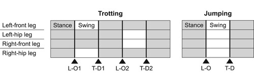
Numerical experiments on the whole-body optimal control of a quadrupedal robot ANYmal (Hutter et al., Citation2017) were conducted to demonstrate the efficiency of the proposed method in practical and complicated examples. A trotting motion with a step length of 0.15 m and aggressive jumping motion with a jump length of 0.8 m also investigated. The contact patterns of the trotting and jumping motions are shown in Figure . The state equation of the robot switched based on the combination of the support feet, that is, it switched when the feet lifted off from the ground or touched down onto the ground. Therefore, the trotting motion had four switches and the jump motion had two switches over the horizon, as shown in Figure . The lift-off did not include the state jump or the switching condition, but the touch-down included both (Farshidian et al., Citation2017; Li & Wensing, Citation2020; Schultz & Mombaur, Citation2010). The switching condition was treated using the proposed method in Section 5.1: the switching conditions were the position constraints on the foot whose Jacobian took the form of (Equation36(36)
(36) ), and the state equation of the robot under an acceleration-level rigid-contact constraint took the form of (Equation35
(35)
(35) ). The details of the above formulations can be found in Li and Wensing (Citation2020); Schultz and Mombaur (Citation2010). Note also that the acceleration-level contact-consistent dynamics of the robot were lifted to improve the convergence speed without changing the structure of the KKT system (Equation10
(10a)
(10a) ) (Katayama & Ohtsuka, Citation2021b). To consider a practical situation, the limitations that were imposed on the joint angles, velocities, and torques were considered to be the inequality constraints. The polyhedral-approximated friction cone constraint was also considered for each contact force expressed in the world frame
as:
(44)
(44) where
is the friction coefficient, which was set as
. Note that the friction cone constraint (Equation44
(44)
(44) ) also switched depending on the active subsystems (that is, depending on the combination of the support feet). The initial and terminal times of the horizon were set as
and
for the trotting problem and
and
for the jumping problem, respectively.
Figure 2. Contact patterns of trotting and jumping motions. Gray and white cells indicate the intervals where the leg is standing and swinging, respectively. Thick lines illustrate the switches of the active subsystems. Black triangles indicate the types of switches (lift-off: L-O, touch-down: T-D).
To design the stage cost of the trotting motion, the state was partitioned into the generalised coordinate and velocity
,
. Additionally, the position (i.e. forward kinematics) of the foot
{Left-front, Left-hip, Right-front, Right-hip} was considered in the world frame
. The stage cost was then designed for the trotting motion, which is expressed as
(45)
(45) where
is the generalised acceleration,
and
are reference values, and
and
are diagonal weight matrices.
was chosen as the generalised coordinate of the standing pose of the robot. We set the desired translational velocity of the floating base of the robot as
and set the other element of
as zero. The plane coordinate of
was set as a middle point of the two successive predefined ground locations of the foot, and its vertical coordinate was set as the desired height of the swing foot. The last term in (Equation45
(45)
(45) ) changed depending on the swing legs, that is, the stage cost also switched as the active subsystem. The terminal cost
and impulse cost
were set as the sums of the first and second terms of (Equation45
(45)
(45) ), respectively. Similarly, the stage cost was designed for the jumping motions, which is expressed as
(46)
(46) In addition, the terminal cost
and impulse cost
were set as the sums of the first and second terms of (Equation46
(46)
(46) ), respectively, but with different weight parameters. The minimum-dwell times in (Equation4e
(4e)
(4e) ) for the trotting motion were set as
and
. The minimum-dwell times were set for the jumping motion as
and
. A large
was set in the jumping motion to sufficiently observe the whole-body motion after touch-down. This was because the optimiser tended to make the touch-down time very close to the end of the horizon to minimise the overall cost of the OCP without a large
.
The proposed algorithms were implemented in C++, and Eigen was used for the linear algebra. The efficient Pinocchio C++ library was used (Carpentier et al., Citation2019) for rigid-body dynamics (Featherstone, Citation2008) and its analytical derivatives (Carpentier & Mansard, Citation2018) to compute the dynamics and its derivatives of the quadrupedal robot. The Gauss-Newton Hessian approximation was used to avoid computing the second-order derivatives of the rigid-body dynamics. The reduced Hessian modifications (Equation27(27)
(27) ) and (Equation28
(28)
(28) ) were used in the proposed Riccati recursion.
and
were chosen using (Equation29
(29)
(29) ) with
. Only the fraction-to-boundary rule (Nocedal & Wright, Citation2006; Wächter & Biegler, Citation2006) was used for the step-size selection. The barrier parameter was fixed at
, which is a common suboptimal MPC setting (Wang & Boyd, Citation2010). OpenMP (Dagum & Menon, Citation1998) was used for parallel computing of the KKT system (Equation10
(10a)
(10a) ) in stage-wise and eight threads through the following experiments. These two experiments were conducted on a desktop computer with an octa-core CPU Intel Core i9-9900 @3.10 GHz.
was used for the mesh refinement. The total number of horizon grids was fixed to N = 50 and N = 90 for the trotting and jumping problems, respectively. That is, when grids were added to the mesh-refinement phase, the same number of grids were removed from the other phases. The proposed method converged when the
norm of the KKT residual was smaller than a sufficiently small threshold
and each
was smaller than
. Mesh refinement was performed when the
norm of the KKT residual became moderately small (smaller than 0.1). After the mesh refinement, the iterates
,
, and
were reconstructed by the linear interpolation of these variables that were stored before the mesh refinement. This implementation is available online as a part of our efficient optimal control solvers for robotic systems, called robotoc (Katayama, Citation2020).
6.2.2. Results
The convergence results of the trotting and jumping motions are shown in Figures and , respectively. For the trotting motion that included a mesh-refinement step, the proposed method converged after 40 iterations. The total computational time was 52 ms (1.3 ms per Newton iteration). For the jumping motion that included two mesh-refinement steps, the proposed method converged after 82 iterations. The total computational time was 172 ms (2.1 ms per Newton iteration). The snapshots of the solution trajectory of the aggressive jumping motion are shown in Figure , and the time histories of the contact forces of the four feet in the jumping motion are shown in Figure . We can see that the contact forces lie inside the friction cone constraints throughout the jumping motion. These two figures show that the friction cone constraints (Equation44(44)
(44) ) were active at time intervals immediately before and after the jumping, and the solution strictly satisfied the constraints.
Figure 3. Convergence of the proposed method for the trotting motion of a quadrupedal robot: (a) switching instants and (b) norm of the residual in the perturbed KKT conditions over the iterations. Vertical dotted lines indicate that the mesh refinement was performed.
Figure 4. Convergence of the proposed method for the jumping motion of the quadrupedal robot: (a) switching instants and (b) norm of the residual in the perturbed KKT conditions over the iterations. Vertical dotted lines indicate that the mesh refinement was carried out.
Figure 5. Snapshots of solution trajectory of the whole-body optimal control of ANYmal's 0.8 m aggressive jumping motion. The yellow arrows and blue polyhedrons represent the contact forces and friction cone constraints, respectively, which are not illustrated while the robot is flying.
Figure 6. Time histories of the contact force expressed in the world frame of each leg in the jumping motion. The infeasible regions of
(solid lines) and
(dashed lines) due to the friction cone constraints are the filled gray hatches. The infeasible region of
(dash-dotted lines) is in the lower-half of each plot.
![Figure 6. Time histories of the contact force expressed in the world frame [fxfyfz] of each leg in the jumping motion. The infeasible regions of fx (solid lines) and fy (dashed lines) due to the friction cone constraints are the filled gray hatches. The infeasible region of fz≥0 (dash-dotted lines) is in the lower-half of each plot.](/cms/asset/d68ba47e-6e09-477f-accb-33ab2a18dbca/tcon_a_2227285_f0006_oc.jpg)
The above results showed that the proposed method could achieve fast convergence and computational times per Newton iteration, even for large-scale (36-dimensional state, 12-dimensional control input) and complicated problems. In MPC, the shorter length of the horizon and smaller number of discretization grids can typically be considered, and warm-starting can be leveraged. For example, the computational time per Newton iteration for the trotting problem can be expected to be less than half of 1.3 ms if the number of grids was reduced to 20. Therefore, the proposed method is a promising approach that can achieve the whole-body MPC of robotics systems having rigid contacts within a milliseconds-range sampling time.
7. Conclusion
This study proposed an efficient Newton-type method for optimal control of switched systems under a given mode sequence. A direct multiple-shooting method with adaptive mesh refinement was formulated to guarantee the local convergence of the Newton-type method for the NLP. A dedicated structure-exploiting Riccati recursion algorithm was proposed that performed the Newton-type method for the NLP with the linear time-complexity of the total number of discretization grids. Moreover, the proposed method could always solve the KKT systems if the solution was sufficiently close to a local minimum. Conversely, general QP solvers cannot be guaranteed to solve the KKT systems because the Hessian matrix is inherently indefinite. Moreover, to enhance the convergence, a modification on the reduced Hessian matrix was proposed using the nature of the Riccati recursion algorithm as the dynamic programming for a QP subproblem. A numerical comparison was conducted with off-the-shelf solvers and demonstrated that the proposed method was up to two orders of magnitude faster. Whole-body optimal control of quadrupedal gaits was also investigated and it was demonstrated that the proposed method could achieve the whole-body MPC of robotic systems with rigid contacts.
A possible future extension of the proposed method is OCPs with free final time, including minimum-time OCPs (Bryson & Ho, Citation1975), because the NLP structure of such problems is expected to be similar to the proposed formulation.
Disclosure statement
No potential conflict of interest was reported by the author(s).
Data availability statement
The data of 6.2 can be reproduced by our open-source software https://github.com/mayataka/robotoc. Other data that support the findings of this study are also available from the corresponding author, Sotaro Katayama, upon reasonable request.
Additional information
Funding
References
- Amestoy, P., Duff, I. S., L'Excellent, J. Y., & Koster, J. (2001). A fully asynchronous multifrontal solver using distributed dynamic scheduling. SIAM Journal on Matrix Analysis and Applications, 23(1), 15–41. https://doi.org/10.1137/S0895479899358194
- Andersson, J. A. E., Gillis, J., Horn, G., Rawlings, J. B., & Diehl, M. (2019). CasADi – a software framework for nonlinear optimization and optimal control. Mathematical Programming Computation, 11(1), 1–36. https://doi.org/10.1007/s12532-018-0139-4
- Belotti, P., Kirches, C., Leyffer, S., Linderoth, J., Luedtke, J., & Mahajan, A. (2013). Mixed-integer nonlinear optimization. Acta Numerica, 22, 1–131. https://doi.org/10.1017/S0962492913000032
- Bertsekas, D. P. (2005). Dynamic programming and optimal control (3rd ed.). Athena Scientific.
- Betts, J. T. (2010). Practical methods for optimal control and estimation using nonlinear programming (2nd ed.). Cambridge University Press.
- Bock, H., & Plitt, K. (1984). A multiple shooting algorithm for direct solution of optimal control problem. 9th IFAC World Congress, 17(2), 1603–1608. https://doi.org/10.1016/S1474-6670(17)61205-9
- Bryson, A. E., & Ho, Y. C. (1975). Applied optimal control: optimization, estimation, and control. CRC Press.
- Bürger, A., Zeile, C., Altmann-Dieses, A., Sager, S., & Diehl, M. (2019). Design, implementation and simulation of an MPC algorithm for switched nonlinear systems under combinatorial constraints. Journal of Process Control, 81, 15–30. https://doi.org/10.1016/j.jprocont.2019.05.016
- Carpentier, J., & Mansard, N. (2018). Analytical derivatives of rigid body dynamics algorithms. In Robotics: science and systems (RSS 2018) (p. hal-01790971v2f).
- Carpentier, J., Saurel, G., Buondonno, G., Mirabel, J., Lamiraux, F., Stasse, O., & Mansard, N. (2019). The Pinocchio C++ library – a fast and flexible implementation of rigid body dynamics algorithms and their analytical derivatives The Pinocchio C++ library – A fast and flexible implementation of rigid body dynamics algorithms and their analytical derivatives. In International symposium on system integration (SII) (pp. 614–619).
- Dagum, L., & Menon, R. (1998). OpenMP: an industry-standard API for shared-memory programming. IEEE Computational Science & Engineering, 5(1), 46–55. https://doi.org/10.1109/99.660313
- Di Carlo, J., Wensing, P. M., Katz, B., Bledt, G., & Kim, S. (2018). Dynamic locomotion in the MIT cheetah 3 through convex model-predictive control. In 2018 IEEE/RSJ international conference on intelligent robots and systems (IROS) (pp. 1–9).
- Diehl, M., Bock, H. G., & Schlöder, J. P. (2005). A real-time iteration scheme for nonlinear optimization in optimal feedback control. SIAM Journal on Control and Optimization, 43(5), 1714–1736. https://doi.org/10.1137/S0363012902400713
- Farshidian, F., Jelavic, E., Satapathy, A., Giftthaler, M., & Buchli, J (2017). Real-time motion planning of legged robots: a model predictive control approach. In 2017 IEEE-RAS 17th international conference on humanoid robotics (Humanoids) (pp. 577–584).
- Farshidian, F., Kamgarpour, M., Pardo, D., & Buchli, J. (2017). Sequential linear quadratic optimal control for nonlinear switched systems. IFAC-PapersOnLine, 50(1), 1463–1469. https://doi.org/10.1016/j.ifacol.2017.08.29120th IFAC World Congress.
- Featherstone, R. (2008). Rigid body dynamics algorithms. Springer.
- Ferreau, H. J., Kirches, C., Potschka, A., Bock, H. G., & Diehl, M. (2014). qpOASES: a parametric active-set algorithm for quadratic programming. Mathematical Programming Computation, 6(4), 327–363. https://doi.org/10.1007/s12532-014-0071-1
- Fu, J., & Zhang, C. (2021). Optimal control of path-constrained switched systems with guaranteed feasibility. IEEE Transactions on Automatic Control, 67(3), 1342–1355. https://doi.org/10.1109/TAC.2021.3071035
- Grandia, R., Taylor, A. J., Ames, A. D., & Hutter, M. (2021). Multi-Layered Safety for Legged Robots via Control Barrier Functions and Model Predictive Control. In 2021 IEEE international conference on robotics and automation (ICRA) (pp. 8352–8358).
- Guennebaud, G., & Jacob, B. (2010). Eigen v3. http://eigen.tuxfamily.org.
- Hutter, M., Gehring, C., Lauber, A., Gunther, F., Bellicoso, C. D., Tsounis, V., Fankhauser, P., Diethelm, R., Bachmann, S., Bloesch, M., Kolvenbach, H., Bjelonic, M., Isler, L., & Meyer, K. (2017). ANYmal – toward legged robots for harsh environments. Advanced Robotics, 31(17), 918–931. https://doi.org/10.1080/01691864.2017.1378591
- Jenelten, F., Miki, T., Vijayan, A. E., Bjelonic, M., & Hutter, M. (2020). Perceptive locomotion in rough terrain – online foothold optimization. IEEE Robotics and Automation Letters, 5, 5370–5376. https://doi.org/10.1109/LSP.2016.
- Johnson, E. R., & T. D. Murphey (2011). Second-Order switching time optimization for nonlinear time-varying dynamic systems. IEEE Transactions on Automatic Control, 56(8), 1953–1957. https://doi.org/10.1109/TAC.2011.2150310
- Jung, M. N., Kirches, C., & Sager, S. (2013). On perspective functions and vanishing constraints in mixed-integer nonlinear optimal control. In G. R. M. Jünger (Ed.), Facets of combinatorial optimization (pp. 387–417). Springer.
- Katayama, S. (2020). robotoc. https://github.com/mayataka/robotoc.
- Katayama, S., Doi, M., & Ohtsuka, T (2020). A moving switching sequence approach for nonlinear model predictive control of switched systems with state-dependent switches and state jumps. International Journal of Robust and Nonlinear Control, 30(2), 719–740. https://doi.org/10.1002/rnc.v30.2
- Katayama, S., & Ohtsuka, T. (2021a). Efficient Riccati recursion for optimal control problems with pure-state equality constraints. arXiv:2102.09731.
- Katayama, S., & Ohtsuka, T. (2021b). Lifted contact dynamics for efficient direct optimal control of rigid body systems with contacts. arXiv:2108.01781.
- Katayama, S., & Ohtsuka, T. (2021c). Riccati recursion for optimal control problems of nonlinear switched systems. In Proceedings of the 7th IFAC conference on nonlinear model predictive control 2021 (NMPC) (p. 18).
- Kuindersma, S., Deits, R., Fallon, M., Valenzuela, A., Dai, H., Permenter, F., Koolen, T., Marion, P., & Tedrake, R. (2016). Optimization-based locomotion planning, estimation, and control design for the Atlas humanoid robot. Autonomous Robots, 40, 429–455. https://doi.org/10.1007/s10514-015-9479-3
- Li, H., & Wensing, P. M. (2020). Hybrid systems differential dynamic programming for whole-body motion planning of legged robots. IEEE Robotics and Automation Letters, 5(4), 5448–5455. https://doi.org/10.1109/LSP.2016.
- Mastalli, C., Havoutis, I., Focchi, M., Caldwell, D. G., & Semini, C. (2020). Motion planning for quadrupedal locomotion: coupled planning, terrain mapping, and whole-body control. IEEE Transactions on Robotics, 36(6), 1635–1648. https://doi.org/10.1109/TRO.8860
- Messerer, F., Baumgärtner, K., & Diehl, M. (2021). Survey of sequential convex programming and generalised Gauss-Newton methods. Citation: ESAIM: Proceedings and Surveys, 71(1), 64–88. https://doi.org/10.1051/proc/202171107
- Nocedal, J., & Wright, S. J. (2006). Numerical optimization (2nd ed.). Springer.
- Nurkanović, A., Albrecht, S., & Diehl, M. (2020). Limits of MPCC formulations in direct optimal control with nonsmooth differential equations. In 2020 European control conference (ECC) (pp. 2015–2020).
- Ohtsuka, T. (2004). A continuation/GMRES method for fast computation of nonlinear receding horizon control. Automatica, 40(4), 563–574. https://doi.org/10.1016/j.automatica.2003.11.005
- Patterson, M. A., & Rao, A. V. (2014). GPOPS-II: A MATLAB software for solving multiple-phase optimal control problems using hp-Adaptive Gaussian quadrature collocation methods and sparse nonlinear programming. ACM Transactions on Mathematical Software, 41(1), 1–37. https://doi.org/10.1145/2558904
- Posa, M., Cantu, C., & Tedrake, R. (2014). A direct method for trajectory optimization of rigid bodies through contact. The International Journal of Robotics Research, 33(1), 69–81. https://doi.org/10.1177/0278364913506757
- Quirynen, R., Houska, B., Vallerio, M., Telen, D., Logist, F., Van Impe, J., & Diehl, M. (2014). Symmetric algorithmic differentiation based exact Hessian SQP method and software for Economic MPC. In 53rd IEEE conference on decision and control (CDC) (pp. 2752–2757).
- Rao, C., Wright, S. J., & Rawlings, J. B. (1998). Application of interior-point methods to model predictive control. Journal of Optimization Theory and Applications, 99(3), 723–757. https://doi.org/10.1023/A:1021711402723
- Rawlings, K., Mayne, D. Q., & Diehl, M. (2017). Model predictive control: theory, computation, and design. Nob Hill Publishing, LCC.
- Robuschi, N., Zeile, C., Sager, S., & Braghin, F. (2021). Multiphase mixed-integer nonlinear optimal control of hybrid electric vehicles. Automatica, 123, 109325. https://doi.org/10.1016/j.automatica.2020.109325
- Sager, S., Jung, M. N., & Kirches, C. (2011). Combinatorial integral approximation. Mathematical Methods of Operations Research, 73, 363–380. https://doi.org/10.1007/s00186-011-0355-4
- Schultz, G., & Mombaur, K. (2010). Modeling and optimal control of human-like running. IEEE/ASME Transactions on Mechatronics, 15(5), 783–792. https://doi.org/10.1109/TMECH.2009.2035112
- Sideris, A., & Rodriguez, L. A. (2011). A Riccati approach for constrained linear quadratic optimal control. International Journal of Control, 84(2), 370–380. https://doi.org/10.1080/00207179.2011.555883
- Stellato, B., Banjac, G., Goulart, P., Bemporad, A., & Boyd, S. (2020). OSQP: an operator splitting solver for quadratic programs. Mathematical Programming Computation, 12(4), 637–672. https://doi.org/10.1007/s12532-020-00179-2
- Stellato, B., Ober-Blöbaum, S., & Goulart, P. J. (2017). Second-order switching time optimization for switched dynamical systems. IEEE Transactions on Automatic Control, 62(10), 5407–5414. https://doi.org/10.1109/TAC.2017.2697681
- Wächter, A., & Biegler, L. (2006). On the implementation of an interior-point filter line-search algorithm for large-scale nonlinear programming. Mathematical Programming, 106, 25–57. https://doi.org/10.1007/s10107-004-0559-y
- Wang, Y., & Boyd, S. (2010). Fast model predictive control using online optimization. IEEE Transactions on Control Systems Technology, 18(2), 267–278. https://doi.org/10.1109/TCST.2009.2017934
- Xu, X., & Antsaklis, P. J. (2002). Optimal control of switched systems via non-linear optimization based on direct differentiations of value functions. International Journal of Control, 75(16-17), 1406–1426. https://doi.org/10.1080/0020717021000023825
- Xu, X., & Antsaklis, P. J. (2004). Optimal control of switched systems based on parameterization of the switching instants. IEEE Transactions on Automatic Control, 49(1), 2–16. https://doi.org/10.1109/TAC.2003.821417
- Yunt, K. (2011). An augmented lagrangian based shooting method for the optimal trajectory generation of switching lagrangian systems. Dynamics of Continuous, Discrete and Impulsive Systems Series B: Applications and Algorithms, 18(5), 615–645. https://www.researchgate.net/profile/Kerim-Yunt/publication/255621657_An_augmented_Lagrangian_based_shooting_method_for_the_optimal_trajectory_generation_of_switching_Lagrangian_systems/links/56c9960908ae5488f0d904e7/Anaugmented-Lagrangian-based-shooting-method-for-the-optimal-trajectory-generation-of-switching-Lagrangian-systems.pdf
- Zanelli, A., Domahidi, A., Jerez, J., & Morari, M. (2020). FORCES NLP: an efficient implementation of interior-point methods for multistage nonlinear nonconvex programs. International Journal of Control, 93(1), 13–29. https://doi.org/10.1080/00207179.2017.1316017