Modelling and analysis of a cooperative production network

Abstract

In this study, we examine the cooperative production business model for a group of producers serving their own customers and also have access to external customers who can make an agreement to buy products at a lower price if a desired service level can be guaranteed. When the producers cannot meet the desired service level requirement of the external customers at the offered price on their own, they participate in a cooperative network. The network consolidates the external customers for its members and routes an arriving external customer to one of the participants. We determine the optimal production and rationing policies for each participating manufacturer as well as the optimal routing policy for the network. We also propose an accurate approximate method to analyse a network with a high number of homogeneous producers using a single queue approximation method. We show that, based on the parameters of the producers and the external market, the network can provide the desired service level for the external customers at the offered price and makes all the members increase their profit by better utilising their capacity and serving more external customers.

Keywords:

• cooperation
• cloud manufacturing
• dynamic manufacturing network
• inventory rationing
• demand classes
• single queue approximation

1. Introduction

In response to the economic condition and competition in the business environment, producers began using cooperation-based business models to utilise their capacity effectively and access more customers. Different mechanisms enable producers to work together and share resources. These mechanisms facilitate cooperation among different producers and provide more efficient services at a lower cost. Cooperation among producers may allow cooperating members to benefit from cost advantages due to economies of scale effects, utilisation improvements due to resource pooling, and flexibility enrichments among other benefits.

Since several manufacturing enterprises have shown great interest for creating such networks in order to meet emerging market needs and business opportunities, manufacturing networks have become an attractive topic for the researchers in the recent years. Different terms such as Dynamic Manufacturing Networks (Papakostas et al. 2013; Ferreira et al. 2014; Ivanov et al. 2016) and Virtual Manufacturing Networks (Wadhwa, Mishra, and Chan 2009) have been also used in addition to Collaborative Manufacturing Networks (Danilovic and Winroth 2005).

With the advances in technology, the producers can establish these networks easily. The Cloud Manufacturing platforms allow producers to cooperate and interact with their customers in a more effective way. The Cloud Manufacturing is defined as a manufacturing model that exploits on-demand access to a shared collection of distributed manufacturing resources to form temporary production lines which enhance efficiency and allow for optimal resource loading in response to variable customer's demand (Li et al. 2010; Wu et al. 2013; Zhang et al. 2014). It is expected that connecting a wide range of producers in a cloud manufacturing network will allow the network to allocate the orders dynamically among the members and make it possible to fulfil orders that were not economically viable when the producers work independently. Developing business models that describe how manufacturing services are provided and how they can be deployed and paid is important to realise the expected benefits of cooperation (Putnik 2012; Wu et al. 2013; Ren et al. 2014). An example for this kind of setting is MFG.com which is one of the largest contract manufacturing marketplaces and enables the customers to access manufacturers though an easy to use on-line platform.

Our study is motivated from such a situation that a group of producers can cooperate in a network setting. These manufacturers produce a single product for their own inventories and serve their own customers. They also have access to another group of customers, referred as the external customers, who offer a lower price for the products compared to the producers' own customers and also require a specific service level. For example, consider that a producer wants to use his excess capacity to produce for other companies as a private label supplier. In order to be accepted as a private label supplier, he should meet the service level requirements of the company that will use the producer as a supplier. If a producer can meet the service level requirement of the external customers in an economically viable way, these customers bring additional business and allow the producer to utilise his resources more effectively. However, due to the service level requirements and also the lower price, these customers are not usually served by individual producers.

The cooperative network we analyse consolidates the orders from the external customers and routes the orders to available producers in such a way that the desired service level requirement of the external customers is met. Cooperation of producers in this network is expected to meet the desired service level at a lower cost and therefore generates additional business to its members and utilises their resources more effectively.

In this paper, our main objective is to answer the following main question: What is the benefit of joining a cooperative network depending on the characteristics of the producers and the external customers? In order to answer this question, we also answer the following questions regarding the operation of this cooperative network: How do the producers manage their production and decide on meeting the demand from different groups of customers?; and How do the producers decide on joining the cooperative network or not?

We model the system with exponentially distributed production times and exponential order inter-arrival times as a Continuous time Markov chain to evaluate the performance of the system when the production and sales decisions of the producers and the routing decision of the network are given optimally. For the network operation with dynamic routing policy and heterogeneous producers, we solve an LP formulation of the stochastic dynamic programme to determine the optimal production, sales, and routing policies. Moreover, for the network operation with dynamic routing policy and homogeneous producers, we develop an approximation method that allows us to analyse the cooperative network with a high number of members. We determine whether it is beneficial for a producer to join the cooperative network by comparing the expected profit of operating independently with the expected profit of participating in the cooperative network. We show that the cooperative network can increase the profits of the producers significantly for the high values of the requested service level.

The organisation of the remaining parts of this paper is as follows: We review the pertinent literature in Section 2. In Section 3, we present the model and its assumptions. Then we analyse independent operation as the first step in Section 4. In Section 5, we give the analysis of the model for dynamic cooperative network. After the exact analysis of the optimal policies, we perform an approximate investigation for a cooperative network with a large number of identical participants in Section 6. Based on our analysis, numerical results are given in Section 7 and we specify some managerial insights in Section 8. Finally, Section 9 is devoted to concluding remarks.

2. Past work

Our study is related to the production control with multiple demand classes literature and also to the cooperation in supply chain literature.

2.1. Production control with multiple demand classes

Whenever the limited capacity of a supplier is to be shared among multiple groups of customers with different profit margins, it may be more profitable for the supplier to reject an arriving customer in order to reserve the available inventory for upcoming more profitable customers. In addition, if the production capacity is limited, the producer should decide on how to control production and how to serve different demand classes.

One of the earliest works in this area is presented by Topkis (1968), who developed an optimal stock rationing problem for an uncapacitated system. This research has been extended with different kinds of assumption in various directions, e.g. (Nahmias and Demmy 1981; Cohen, Kleindorfer, and Lee 1988; Frank, Zhang, and Duenyas 2003). Deshpande, Cohen, and Donohue (2003) give a detailed review of this literature.

Ha (1997a) analysed the optimal rationing and production policy of a lost-sale manufacturing system using a queuing-based model. Ha (1997b) also expands this work for a system with two different classes of customers and backorder. Véricourt, Karaesmen, and Dallery (2002) generalised this problem for multiple classes of customers. Véricourt, Karaesmen, and Dallery (2001) also performed a comparison among three general kinds of control policies for a make-to-stock production system with multiple classes of customers and showed that the multi-level rationing policy always outperforms the other two policies.

During the recent years, the rationing policies have been investigated for various systems with different processing time distributions (Lee and Hong 2003; Gayon, DeVericourt, and Karaesmen 2009), with batch ordering (Huang and Iravani 2007; Pang, Shen, and Cheng 2014), with batch arrivals (Çil, Ormeci, and Karaesmen 2009), among others (Carr and Duenyas 2000; Duran et al. 2007; Gayon, Benjaafar, and DeVéricourt 2009; Liu et al. 2015).

2.2. Cooperation on production, inventory, and sales

The benefits of pooling capacity and inventory have been shown in different studies. Benjaafar, Cooper, and Kim (2005) examined inventory pooling in production-inventory systems and showed that all characteristics of the structure play important roles in determining precisely how valuable pooling might be. Yu, Benjaafar, and Gerchak (2015) presented models to study the benefit of capacity pooling among independent service firms and showed that it can reduce total cost and all firms can benefit under an appropriate cost-sharing scheme. Tan (2006) presented a stochastic model to analyse cooperation of producers on production capacity. An auction-based allocation method is proposed to distribute large orders and additional benefits among independent producers. Demand allocation problem in a system with multiple inventory locations is also studied by Benjaafar, ElHafsi, and Véricourt (2004) and Benjaafar et al. (2008). In this line of research, the emphasis has been on the capacity and inventory management models proposed for the pooled inventory.

In addition to cooperation on capacity and pooling inventory, companies can also cooperate in marketing and sales activities. Using empirical data, Bucklin and Sengupta (1993) identify situations in which marketing cooperation are most successful and Swaminathan and Moorman (2009) explore whether such cooperation indeed adds value to the firms. Akçay and Tan (2008) examine an assortment-based cooperation among independent firms and show that such a cooperation scheme between symmetric single product firms is always beneficial, whereas a threshold-type criterion should be satisfied so that assortment-based cooperation is beneficial for asymmetric firms. However, their model inherently assumes that firms do not have any capacity limitations. Tan and Akçay (2014) extended this model to capture the effects of capacity limitations on benefits of assortment-based cooperation in a stochastic setting.

While there are recent papers on production networks, virtual enterprises and cloud manufacturing, none of these studies uses a detailed operational model to discuss cooperation-based business models under service level constraint. We consider showing the benefits of a cooperation-based business model for a cooperative network by analysing a detailed operational model and examining optimal control policies jointly as the main contribution of this study. In order to analyse the detailed operational model, we investigate the optimal production, rationing, and routing decisions jointly and show the structure of the optimal policies computationally. We also developed an accurate approximation method to analyse the system with a high number of homogeneous producers which reduces the computational effort very much and shows very high accuracy compared to the exact solution.

3. Model description

We consider N production facilities that produce a single product to their stocks and face with two different groups of customers: their own customers and external customers.

Production Facilities. The production time for Producer i is assumed to be exponentially distributed with mean ${\mu }_i^{-1}$, $i=\{1,\dots ,N\}$ for analytical tractability. When a demand arrives, it is either satisfied immediately from the on-hand inventory or is rejected and lost. The service level is defined based on the fill rate. The corresponding unit inventory holding cost for each producer is $h_i$. The production costs are the same for both classes of customers and set to zero by scaling the prices accordingly.

Customer Demand. The first group of customers is referred as the manufacturers' own customers. Producer i's own customers arrive according to a Poisson process with an arrival rate of ${\lambda }_i$ (${\lambda }_i<{\mu }_i$) and pay a price of $p_i$. The requests of the manufacturers' own customers are satisfied by them directly and the service level received by manufacturer i's own customers is ${\gamma }_i^o$.

The second group is referred as the external customers. We assume that the demand of the external customers for all producers are generated from the same class of customers, e.g. from the pool of companies that are in search of suppliers for private-label production. They expect a desired service level (fill rate) of γ from the manufacturers. Producer i's external customers arrive according to a Poisson process with rate ${\lambda }_{ei}$. They pay a lower price of $p_{ei}$, $p_i>p_{ei}$, and the business offer introduced by the external customers is (${\lambda }_{ei}$, $p_{ei}$, γ). The manufacturers accept the offer from this group of customers only if they can provide the desired service level in a profitable way. Otherwise, they reject the external offer since they cannot meet their service level expectation, and continue their operation by serving only their own customers.

In the period of time that a producer accepts the external business offer, he will serve his own customers with a higher or at least equal service level as the external customers, i.e., ${\gamma }_i^o\ge \gamma$.

Figure 1(a) depicts the independent operation of a producer.

Figure 1. (a) Accepting external customers directly, (b) Cooperative network for external sales.

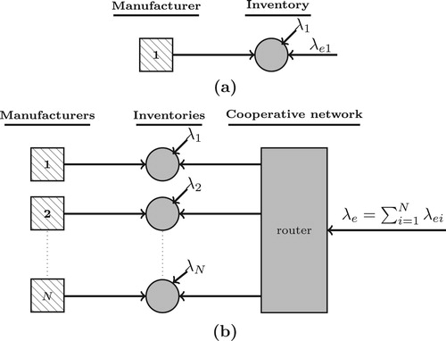
Network. A producer can participate in a cooperative network with other manufacturers. The network consolidates the external customers of all the members and serves them by routing an arriving external demand originated from the external customers of one of the members to one of the producers in the network. The total arrival rate of the external customers to the network is ${\lambda }_e=\sum _{i=1}^N{\lambda }_{ei}$. Note that in the network operation, each member continues to satisfy his own customers demand independently.

We analyse the operation of cooperative network with dynamic routing policy where the producers share their inventory levels continuously with the network. The producers also share their capacity, price, cost, and demand information with the network. The optimal production, rationing and routing policies should be determined to understand the operation of the network. The whole profit obtained in the cooperative network is shared among participating manufacturers in a way that each of them earn more profit in comparison to independent operation. In this study, we will focus on the effect of network in the total profit increase and we assume that the network use side payment to share profit among the members. We also exclude the competition and interoperability between the partners and leave them for the future work.

The parameters for the independent (no cooperation) and cooperation in the network are differentiated by using subscript j, $j\in \{nc,cd\}$, where nc stands for the independent (no cooperation case) and cd stands for cooperation in the cooperative network under the dynamic routing policy. Accordingly, the inventory level for Producer i operating independently is defined by $I_{n{c}_i}$. In the network-based operation, the inventory level of Producer i is defined by $I_{c{d}_i}$.

Figure 1(b) shows the schematic of the cooperative network.

4. Independent operation (no cooperation case)

Since there is a service level constraint for the external demand in our setting, an independent producer should make a decision to accept or reject the external business offer (${\lambda }_{ei}$, $p_{ei}$, γ). When the business offer is accepted, the producer should provide the desired service level for the external customers. Due to this reason, satisfying external offer may lead to a profit decrease. In this case, the producer rejects the external customers and sells the products only to his own customers. However, if the producer can satisfy the external customers' desired service level in a profitable way, he accepts the external business offer.

Independent operation when the external business offer is accepted. Ha (1997a) studied a single-item production system with several demand classes and lost sales using a multi-class $M/M/1$ queue model. It is shown that the optimal production policy is base stock policy and for each class of demand, there is an admission threshold level at or below which it is optimal to start rejecting this class of demand in anticipation of future arrival of more profitable demands.

Accordingly, Producer i operates with a base-stock level ($S_{{nc}_i}$) to decide whether to produce, and with a rationing level ($R_{{nc}_i}$) to decide whether to satisfy an arriving external demand. Whenever Producer i accepts external customers, the profit rate function is defined as follows: (1) ${\mathrm{\Pi }}_{{nc}_i}^{accept}={\lambda }_{i}Pr(I_{{nc}_i}>0)p_i+{\lambda }_{ei}Pr(I_{{nc}_i}>R_{{nc}_i})p_{ei}-h_i{\overline{I}}_{{nc}_i}.$(1) In this equation, the first term shows that Producer i makes a revenue of $p_i$ from an arrival of its own customers as long as the finished goods inventory is not empty. $Pr(I_{{nc}_i}>0)$ is the stationary probability that the inventory level $I_{{nc}_i}$ is greater than zero and it defines the offered service level for own customers: ${\gamma }_{{nc}_i}^o=Pr(I_{{nc}_i}>0)$. The second term shows that whenever the inventory level is greater than the determined rationing level, it accepts an additional demand from the external customers and makes a revenue of $p_{ei}$ per unit. $Pr(I_{{nc}_i}>R_{{nc}_i})$ is the stationary probability that the inventory level $I_{{nc}_i}$ is greater than the rationing level $R_{{nc}_i}$. Finally, the last term depicts the inventory holding cost. ${\overline{I}}_{{nc}_i}$ is the expected level of inventory for producer i.

The traffic intensity at producer i due to his own customers is defined by ${\rho }_i={\lambda }_i/{\mu }_i$. Also, whenever Producer i accepts the external business offer, the traffic intensity due to the all customers (own customers and external customers) is given by ${\xi }_{{nc}_i}=({\lambda }_i+{\lambda }_{ei})/{\mu }_i$. The performance measures of the system are determined from the steady-state probabilities as follows: (2) $\begin{array}{rl}Pr(I_{{nc}_i}>R_{{nc}_i})& =1-\frac{(1-{\xi }_{{nc}_i}){\xi }_{{nc}_i}^{S_{{nc}_i}-R_{{nc}_i}}(1-{\rho }_i^{R_{{nc}_i}+1})}{(1-{\rho }_i)(1-{\xi }_{{nc}_i}^{S_{{nc}_i}-R_{{nc}_i}})+(1-{\xi }_{{nc}_i}){\xi }_{{nc}_i}^{S_{{nc}_i}-R_{{nc}_i}}(1-{\rho }_i^{R_{{nc}_i}+1})},\end{array}$(2) (3) $\begin{array}{rl}Pr(I_{{nc}_i}>0)& =1-\frac{(1-{\xi }_{{nc}_i})(1-{\rho }_i){\xi }_{{nc}_i}^{S_{{nc}_i}-R_{{nc}_i}}{\rho }_i^{R_{{nc}_i}}}{(1-{\rho }_i)(1-{\xi }_{{nc}_i}^{S_{{nc}_i}-R_{{nc}_i}})+(1-{\xi }_{{nc}_i}){\xi }_{{nc}_i}^{S_{{nc}_i}-R_{{nc}_i}}(1-{\rho }_i^{R_{{nc}_i}+1})},\end{array}$(3) (4) $\begin{array}{rl}{\overline{I}}_{{nc}_i}& =E\left[I_{{nc}_i}\right(t\left)\right]\\ & =S_{{nc}_i}-\frac{\left({\xi }_{{nc}_i}\right(1-{\rho }_i\left)/\right(1-{\xi }_{{nc}_i}\left)\right)(1-{\xi }_{{nc}_i}^{S_{{nc}_i}-R_{{nc}_i}}-(1-{\xi }_{{nc}_i}\left)\right(S_{{nc}_i}-R_{{nc}_i}\left){\xi }_{{nc}_i}^{S_{{nc}_i}-R_{{nc}_i}-1}\right)}{(1-{\rho }_i)(1-{\xi }_{{nc}_i}^{S_{{nc}_i}-R_{{nc}_i}})+(1-{\xi }_{{nc}_i}){\xi }_{{nc}_i}^{S_{{nc}_i}-R_{{nc}_i}}(1-{\rho }_i^{R_{{nc}_i}+1})}\\ & -\frac{{\rho }_i(1-{\xi }_{{nc}_i})/(1-{\rho }_i)}{(1-{\rho }_i)(1-{\xi }_{{nc}_i}^{S_{{nc}_i}-R_{{nc}_i}})+(1-{\xi }_{{nc}_i}){\xi }_{{nc}_i}^{S_{{nc}_i}-R_{{nc}_i}}(1-{\rho }_i^{R_{{nc}_i}+1})}\\ & \times \frac{\left({\xi }_{{nc}_i}/{\rho }_i{)}^{S_{{nc}_i}-R_{{nc}_i}}\right({\rho }_i^{S_{{nc}_i}-R_{{nc}_i}}-{\rho }_i^{S_{{nc}_i}+1}+(1-{\rho }_i)\left[\right(S_{{nc}_i}-R_{{nc}_i}){\rho }_i^{S_{{nc}_i}-R_{{nc}_i}-1}-(S_{{nc}_i}+1\left){\rho }_i^{S_{{nc}_i}}\right])}{(1-{\rho }_i)(1-{\xi }_{{nc}_i}^{S_{{nc}_i}-R_{{nc}_i}})+(1-{\xi }_{{nc}_i}){\xi }_{{nc}_i}^{S_{{nc}_i}-R_{{nc}_i}}(1-{\rho }_i^{R_{{nc}_i}+1})}.\end{array}$(4) Note that Equations (2(2) $\begin{array}{rl}Pr(I_{{nc}_i}>R_{{nc}_i})& =1-\frac{(1-{\xi }_{{nc}_i}){\xi }_{{nc}_i}^{S_{{nc}_i}-R_{{nc}_i}}(1-{\rho }_i^{R_{{nc}_i}+1})}{(1-{\rho }_i)(1-{\xi }_{{nc}_i}^{S_{{nc}_i}-R_{{nc}_i}})+(1-{\xi }_{{nc}_i}){\xi }_{{nc}_i}^{S_{{nc}_i}-R_{{nc}_i}}(1-{\rho }_i^{R_{{nc}_i}+1})},\end{array}$(2) ),(3(3) $\begin{array}{rl}Pr(I_{{nc}_i}>0)& =1-\frac{(1-{\xi }_{{nc}_i})(1-{\rho }_i){\xi }_{{nc}_i}^{S_{{nc}_i}-R_{{nc}_i}}{\rho }_i^{R_{{nc}_i}}}{(1-{\rho }_i)(1-{\xi }_{{nc}_i}^{S_{{nc}_i}-R_{{nc}_i}})+(1-{\xi }_{{nc}_i}){\xi }_{{nc}_i}^{S_{{nc}_i}-R_{{nc}_i}}(1-{\rho }_i^{R_{{nc}_i}+1})},\end{array}$(3) ) and (4(4) $\begin{array}{rl}{\overline{I}}_{{nc}_i}& =E\left[I_{{nc}_i}\right(t\left)\right]\\ & =S_{{nc}_i}-\frac{\left({\xi }_{{nc}_i}\right(1-{\rho }_i\left)/\right(1-{\xi }_{{nc}_i}\left)\right)(1-{\xi }_{{nc}_i}^{S_{{nc}_i}-R_{{nc}_i}}-(1-{\xi }_{{nc}_i}\left)\right(S_{{nc}_i}-R_{{nc}_i}\left){\xi }_{{nc}_i}^{S_{{nc}_i}-R_{{nc}_i}-1}\right)}{(1-{\rho }_i)(1-{\xi }_{{nc}_i}^{S_{{nc}_i}-R_{{nc}_i}})+(1-{\xi }_{{nc}_i}){\xi }_{{nc}_i}^{S_{{nc}_i}-R_{{nc}_i}}(1-{\rho }_i^{R_{{nc}_i}+1})}\\ & -\frac{{\rho }_i(1-{\xi }_{{nc}_i})/(1-{\rho }_i)}{(1-{\rho }_i)(1-{\xi }_{{nc}_i}^{S_{{nc}_i}-R_{{nc}_i}})+(1-{\xi }_{{nc}_i}){\xi }_{{nc}_i}^{S_{{nc}_i}-R_{{nc}_i}}(1-{\rho }_i^{R_{{nc}_i}+1})}\\ & \times \frac{\left({\xi }_{{nc}_i}/{\rho }_i{)}^{S_{{nc}_i}-R_{{nc}_i}}\right({\rho }_i^{S_{{nc}_i}-R_{{nc}_i}}-{\rho }_i^{S_{{nc}_i}+1}+(1-{\rho }_i)\left[\right(S_{{nc}_i}-R_{{nc}_i}){\rho }_i^{S_{{nc}_i}-R_{{nc}_i}-1}-(S_{{nc}_i}+1\left){\rho }_i^{S_{{nc}_i}}\right])}{(1-{\rho }_i)(1-{\xi }_{{nc}_i}^{S_{{nc}_i}-R_{{nc}_i}})+(1-{\xi }_{{nc}_i}){\xi }_{{nc}_i}^{S_{{nc}_i}-R_{{nc}_i}}(1-{\rho }_i^{R_{{nc}_i}+1})}.\end{array}$(4) ) are true when ${\rho }_i\ne 1$ and ${\xi }_{{nc}_i}\ne 1$. The equations for ${\rho }_i=1$ or ${\xi }_{{nc}_i}=1$ are derived in a similar way.

The optimal profit rate of Producer i when he accepts the business offer from the external customers, ${{\mathrm{\Pi }}_{{nc}_i}^{accept}}^{\ast }$, is obtained by maximising Equation (1(1) ${\mathrm{\Pi }}_{{nc}_i}^{accept}={\lambda }_{i}Pr(I_{{nc}_i}>0)p_i+{\lambda }_{ei}Pr(I_{{nc}_i}>R_{{nc}_i})p_{ei}-h_i{\overline{I}}_{{nc}_i}.$(1) ) to determine the optimal base stock level $S_{{nc}_i}^{\ast }$ and the rationing value $R_{{nc}_i}^{\ast }$. The maximisation problem is subject to the external customers' requested service level constraint as follows: (5) $\begin{array}{rl}& {{\mathrm{\Pi }}_{{nc}_i}^{accept}}^{\ast }=\underset{S_{{nc}_i},R_{{nc}_i}}{\max }{\mathrm{\Pi }}_{{nc}_i}^{accept}\\ & \text{subject to:}{\gamma }_{{nc}_i}\ge \gamma .\end{array}$(5) where ${\gamma }_{{nc}_i}=Pr(I_{{nc}_i}>R_{{nc}_i})$ is the offered service level for external customers and ${\gamma }_{{nc}_i}^o\ge {\gamma }_{{nc}_i}$.

Independent operation when the external business offer is rejected. Whenever the producer rejects the external business offer, the expected profit rate function is given as follows: (6) ${\mathrm{\Pi }}_{{nc}_i}^{reject}={\lambda }_i\left(Pr\right(I_{{nc}_i}>0\left)\right)p_i-h_i{\overline{I}}_{{nc}_i}.$(6) The producer chooses the base-stock level $S_{{nc}_i}$ to maximise his profit. Therefore, (7) $\begin{array}{rl}& {{\mathrm{\Pi }}_{{nc}_i}^{reject}}^{\ast }=\underset{S_{{nc}_i}}{\max }{\mathrm{\Pi }}_{{nc}_i}^{reject}.\end{array}$(7) When the external business offer is rejected, we set $S_{{nc}_i}=R_{{nc}_i}$ and ${\rho }_i={\xi }_{{nc}_i}={\lambda }_i/{\mu }_i$ in Equations (2(2) $\begin{array}{rl}Pr(I_{{nc}_i}>R_{{nc}_i})& =1-\frac{(1-{\xi }_{{nc}_i}){\xi }_{{nc}_i}^{S_{{nc}_i}-R_{{nc}_i}}(1-{\rho }_i^{R_{{nc}_i}+1})}{(1-{\rho }_i)(1-{\xi }_{{nc}_i}^{S_{{nc}_i}-R_{{nc}_i}})+(1-{\xi }_{{nc}_i}){\xi }_{{nc}_i}^{S_{{nc}_i}-R_{{nc}_i}}(1-{\rho }_i^{R_{{nc}_i}+1})},\end{array}$(2) )–(4(4) $\begin{array}{rl}{\overline{I}}_{{nc}_i}& =E\left[I_{{nc}_i}\right(t\left)\right]\\ & =S_{{nc}_i}-\frac{\left({\xi }_{{nc}_i}\right(1-{\rho }_i\left)/\right(1-{\xi }_{{nc}_i}\left)\right)(1-{\xi }_{{nc}_i}^{S_{{nc}_i}-R_{{nc}_i}}-(1-{\xi }_{{nc}_i}\left)\right(S_{{nc}_i}-R_{{nc}_i}\left){\xi }_{{nc}_i}^{S_{{nc}_i}-R_{{nc}_i}-1}\right)}{(1-{\rho }_i)(1-{\xi }_{{nc}_i}^{S_{{nc}_i}-R_{{nc}_i}})+(1-{\xi }_{{nc}_i}){\xi }_{{nc}_i}^{S_{{nc}_i}-R_{{nc}_i}}(1-{\rho }_i^{R_{{nc}_i}+1})}\\ & -\frac{{\rho }_i(1-{\xi }_{{nc}_i})/(1-{\rho }_i)}{(1-{\rho }_i)(1-{\xi }_{{nc}_i}^{S_{{nc}_i}-R_{{nc}_i}})+(1-{\xi }_{{nc}_i}){\xi }_{{nc}_i}^{S_{{nc}_i}-R_{{nc}_i}}(1-{\rho }_i^{R_{{nc}_i}+1})}\\ & \times \frac{\left({\xi }_{{nc}_i}/{\rho }_i{)}^{S_{{nc}_i}-R_{{nc}_i}}\right({\rho }_i^{S_{{nc}_i}-R_{{nc}_i}}-{\rho }_i^{S_{{nc}_i}+1}+(1-{\rho }_i)\left[\right(S_{{nc}_i}-R_{{nc}_i}){\rho }_i^{S_{{nc}_i}-R_{{nc}_i}-1}-(S_{{nc}_i}+1\left){\rho }_i^{S_{{nc}_i}}\right])}{(1-{\rho }_i)(1-{\xi }_{{nc}_i}^{S_{{nc}_i}-R_{{nc}_i}})+(1-{\xi }_{{nc}_i}){\xi }_{{nc}_i}^{S_{{nc}_i}-R_{{nc}_i}}(1-{\rho }_i^{R_{{nc}_i}+1})}.\end{array}$(4) ).

Optimal decision to accept or reject external business offer for independent operation. Based on Equations (5(5) $\begin{array}{rl}& {{\mathrm{\Pi }}_{{nc}_i}^{accept}}^{\ast }=\underset{S_{{nc}_i},R_{{nc}_i}}{\max }{\mathrm{\Pi }}_{{nc}_i}^{accept}\\ & \text{subject to:}{\gamma }_{{nc}_i}\ge \gamma .\end{array}$(5) ) and (7(7) $\begin{array}{rl}& {{\mathrm{\Pi }}_{{nc}_i}^{reject}}^{\ast }=\underset{S_{{nc}_i}}{\max }{\mathrm{\Pi }}_{{nc}_i}^{reject}.\end{array}$(7) ), the optimal profit rate function for the independent operation is given as (8) ${\mathrm{\Pi }}_{{nc}_i}^{\ast }=max\{{{\mathrm{\Pi }}_{{nc}_i}^{accept}}^{\ast },{{\mathrm{\Pi }}_{{nc}_i}^{reject}}^{\ast }\}.$(8) The optimal decision of Producer i to accept or reject the external business offer when it operates independently, $g_{n{c}_i}^{\ast }$, is determined by: (9) $g_{n{c}_i}^{\ast }=\left\{\begin{array}{ll}accept& \mathrm{if}{{\mathrm{\Pi }}_{{nc}_i}^{accept}}^{\ast }\ge {{\mathrm{\Pi }}_{{nc}_i}^{reject}}^{\ast }\\ reject& \mathrm{if}{{\mathrm{\Pi }}_{{nc}_i}^{accept}}^{\ast }<{{\mathrm{\Pi }}_{{nc}_i}^{reject}}^{\ast }\end{array}\right..$(9) There might be three reasons for an independent producer to reject an external business offer: The first one is the high utilisation of the producer due to his own customers (ρ). The second reason is the much higher arrival rate of the external customers compared to the production rate. Finally, if the sale price of the external customers is much lower than the price of the producer's own customers, the producer decides reserving more inventory for its own customers due to their higher profit margin. Since there is a service level requirement, the producer will reject the external business offer under a certain selling price defined according to the system parameters.

Figure 2 shows the boundary between the accept and reject regions for two independent producers evaluating the external business offers (${\lambda }_{ei}$, $p_{ei}$, γ). Each producer has a different utilisation level and considers the external business offers for three different values of ${\lambda }_e$. For each value of ${\lambda }_e$ and selling price $p_e$, the independent producers can offer external customers a maximum service level and accept them only if their requested service level is less than or equal to this maximum value. Therefore, all the points over each boundary line with the specified value of ${\lambda }_e$ in Figure 2, defines the region where the producer cannot provide the desired service level for the external customers and prefers to reject them. Consequently, all the points under each boundary line defines the points where the producer is able to provide the desired service level and accepts external business offer.

Figure 2. (a) The boundary between the external customers' accept and reject regions for different values of selling price $p_e$ and requested service level γ when $\rho =0.4$, (b) The boundary between the external customers' accept and reject regions for different values of selling price $p_e$ and requested service level γ when $\rho =0.8$, ($\mu =5,p=100,h=5$).

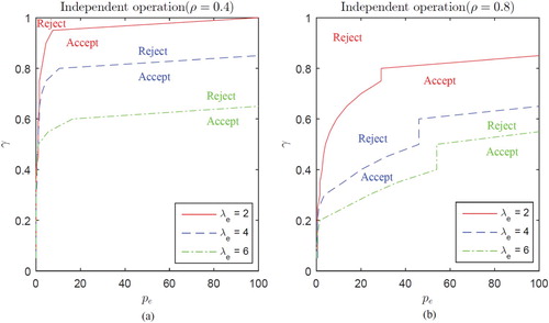
Comparing both graphs in Figure 2(a and b) shows that the accept region is much larger for the producer depicted on the left with a lower level of utilisation ($\rho =0.4$). This means that the producer with a high utilisation could not provide the high service level required for the external offer. The figure also shows that as the arrival rate of the external customers (${\lambda }_e$) increases, the producer decides to offer them a lower service level in order to keep capacity for his own more profitable customers.

As a result, the independent producers may not be able to accept external business offers based on the system parameters. Consequently, losing the potential external offers leads to lower profitability and utilisation. The cooperative network analysed in the following sections is expected to give a solution for this issue by providing the ability to accept the external business offers that are rejected by the producers when they operate independently.

5. Cooperative network with N producers and dynamic routing policy

In order to analyse the operation of the cooperative network with N participating manufacturers, we determine the optimal production, rationing, and routing control policies that maximise the average profit of the system per unit time over an infinite horizon. We employ a Markov decision process framework and due to the memoryless property, the optimal control policy depends only on the current state of the system regardless of time. Thus, we denote the current state of the system by $x=[I_1,I_2,\dots ,I_N]$ where $I_i\in {\mathbb{I}}_i=\{0,1,\dots ,M_i\}$ is the inventory level for producer $i\in \{1,2,\dots ,N\}$ participating in the network and $M_i$ is the maximum number of products in Inventory $I_i$. At any time, the producers should decide on the production policy to produce or to stop production. Let us define these two actions with 1 and 0, respectively, and the action for all members by $u=[u_1,u_2,\dots ,u_N]$ where $u_i$ is the production decision by producer i in the network. When a producer's own customer arrives, it may either be satisfied or rejected. We denote these two actions with 1 and 0 respectively and the action for all members by $f=[f_1,f_2,\dots ,f_N]$ where $f_i$ is the rationing decision of producer i for his own customers. Finally, the network should decide on the routing policy. Let us define the action by $d=\{0,1,2,\dots ,N\}$ where 0 means rejecting the incoming external customer and i means accepting the incoming external demand and sending it to the producer i, $i=1,2,\dots ,N$. Therefore, the control policy is described by $v=\left\{\right(u\left(x\right),f\left(x\right),d\left(x\right)\}$ and $v\in \mathbb{V}$ where $\mathbb{V}$ is the set of all admissible actions.

Given a policy $v\in \mathbb{V}$, let $n_i^o\left(t\right)$ be the number of producer i's own customers who have been accepted by producer i up to time t and $n_i^e\left(t\right)$ be the number of external requests which is satisfied by producer i via the network channel up to time t. We seek to find the optimal control policy v that maximises the following average profit of the system per unit time over an infinite horizon: (10) $\underset{T\to \mathrm{\infty }}{lim}\underset{v\in \mathbb{V}\left(x^0\right)}{sup}\left\{\frac{1}{T}{E}_{x^0}^v\left[\sum _{i=1}^N{\int }_0^T{p}_i{n}_i^o\left(t\right)\mathrm{d}t+\sum _{i=1}^N{\int }_0^T{p}_{ei}{n}_i^e\left(t\right)\mathrm{d}t-\sum _{i=1}^N{\int }_0^T{h}_i{I}_i\left(t\right)\mathrm{d}t\right]\right\}$(10) Where $x^0=[I_1^0,I_2^0,\dots ,I_N^0]$ is the initial inventory level and $E_{x^0}^v$ denotes expectation over demand given an initial inventory level $x^0$.

5.1. Exact analysis of the optimal production, rationing and routing policies of the cooperative network with N participants

In our model, given the current state and decision, any probabilistic statement about the future of the process is completely independent of any information about the history of the process. Therefore, a linear programming formulation can be used to determine the optimal control policy for the Markov Decision Process (Bertsekas et al. 1995; Pietrabissa 2008; Puterman 2014; Bhandari, Scheller-Wolf, and Harchol-Balter 2008; Nadar, Akan, and Scheller-Wolf 2016).

In order to develop a mathematical programming formulation, we construct a discrete-time equivalent of the original system by using the standard tools of uniformisation. To this end, we assume that the time between two consecutive transitions is exponentially distributed with rate $\psi ={\lambda }_e+\sum _{i=1}^N{\lambda }_i+\sum _{i=1}^N{\mu }_i$ which is the maximum transition rate of the system and rescale the time scale of the problem without loss of generality. The decision variable for the linear programming model is defined as $P_{xufd}$, which is the steady-state unconditional probability that the system is in state x, when decisions u,f and d are made.

Let ${\mathrm{\Pi }}_{cd}$ be the expected profit for the producers cooperating in a network with a dynamic routing policy. our objective is maximising the expected long-run profit function, which is written as follows: (11) ${\mathrm{\Pi }}_{cd}=\sum _x\sum _u\sum _f\sum _d{\mathrm{\Pi }}_{xfd}{P}_{xufd}$(11) where (12) $\begin{array}{rl}{\mathrm{\Pi }}_{xfd}& =\sum _{i=1}^N{f}_i{\lambda }_i{p}_i+\sum _{i=1}^{N-1}y(d,i){\lambda }_e{p}_{ei}+w\left(d\right){\lambda }_e{p}_{eN}-\sum _{i=1}^N{I}_i{h}_i,\end{array}$(12) (13) $\begin{array}{rl}y(d,i)& =\frac{\prod _{\begin{array}{c}j=0\\ j\ne i\end{array}}^N(d-j)}{\prod _{\begin{array}{c}j=0\\ j\ne i\end{array}}^N(i-j)},\end{array}$(13) (14) $\begin{array}{rl}w\left(d\right)& =\frac{\prod _{j=0}^{N-1}(d-j)}{N!}.\end{array}$(14) Equation (12(12) $\begin{array}{rl}{\mathrm{\Pi }}_{xfd}& =\sum _{i=1}^N{f}_i{\lambda }_i{p}_i+\sum _{i=1}^{N-1}y(d,i){\lambda }_e{p}_{ei}+w\left(d\right){\lambda }_e{p}_{eN}-\sum _{i=1}^N{I}_i{h}_i,\end{array}$(12) ) is the profit obtained when the system is at state x and the decisions u,f and d are made. The network obtains a profit by selling the product to its own customers when $f_i=1$ and also by selling the product to the external customer from producer $i\in \{1,2,\dots ,N\}$ when d=i. The last term is the inventory holding cost. Equations (13(13) $\begin{array}{rl}y(d,i)& =\frac{\prod _{\begin{array}{c}j=0\\ j\ne i\end{array}}^N(d-j)}{\prod _{\begin{array}{c}j=0\\ j\ne i\end{array}}^N(i-j)},\end{array}$(13) ) and (14(14) $\begin{array}{rl}w\left(d\right)& =\frac{\prod _{j=0}^{N-1}(d-j)}{N!}.\end{array}$(14) ) ensure that the network gains profit by selling the product to the external customer from Producer i when d=i. Hence the mathematical formulation for a general dynamic network with N participating manufacturers is given as follows: (15) $\begin{array}{rl}max{\mathrm{\Pi }}_{cd}& \\ \text{Subject to}& \sum _u\sum _f\sum _d\left[P_{xufd}-\frac{1}{\psi }\left\{\sum _{i=1}^N{u}_i{\mu }_i{P}_{(x-e_i)ufd}+\sum _{i=1}^N{f}_i{\lambda }_i{P}_{(x+e_i)ufd}\right.\right.\end{array}$(15) (16) $\begin{array}{rl}& +\sum _{i=1}^{N-1}y(d,i){\lambda }_e{P}_{(x+e_i)ufd}+w\left(d\right){\lambda }_e{P}_{(x+e_N)ufd}\\ & +P_{xufd}\left.\left.\left(\psi -\sum _{i=1}^N{u}_i{\mu }_i-\sum _{i=1}^N{f}_i{\lambda }_i-\sum _{i=1}^{N-1}y(d,i){\lambda }_e-w\left(d\right){\lambda }_e\right)\right\}\right]=0\mathrm{\forall }x,\\ & \sum _x\sum _u\sum _f\sum _d{P}_{xufd}=1\end{array}$(16) (17) $\begin{array}{rl}& {\mathit{P}}_{\mathit{x}\mathit{u}\mathit{f}\mathit{d}}=0\mathrm{\forall }i,I_i\in \left\{M_i\right\},u_i\in \left\{1\right\},\mathrm{\forall }f,\mathrm{\forall }d,\end{array}$(17) (18) $\begin{array}{rl}& {\mathit{P}}_{\mathit{x}\mathit{u}\mathit{f}\mathit{d}}=0\mathrm{\forall }i,I_i\in \left\{0\right\},f_i\in \left\{1\right\},\mathrm{\forall }u,\mathrm{\forall }d,\end{array}$(18) (19) $\begin{array}{rl}& {\mathit{P}}_{\mathit{x}\mathit{u}\mathit{f}\mathit{d}}=0\mathrm{\forall }i,I_i\in \left\{0\right\},d\in \left\{i\right\},\mathrm{\forall }u,\mathrm{\forall }f,\end{array}$(19) (20) $\begin{array}{rl}& {\mathit{P}}_{\mathit{x}\mathit{u}\mathit{f}\mathit{d}}=0\mathrm{\forall }i,I_i\in \{-1,M_i+1\},\mathrm{\forall }u,\mathrm{\forall }f,\mathrm{\forall }d,\end{array}$(20) (21) $\begin{array}{rl}& \sum _x\sum _u\sum _f\sum _{d=1}^N{P}_{xufd}\ge \gamma .\end{array}$(21) The first two constraints are the balance and the normalisation equations, which yield the steady-state probability values. Equation (17(17) $\begin{array}{rl}& {\mathit{P}}_{\mathit{x}\mathit{u}\mathit{f}\mathit{d}}=0\mathrm{\forall }i,I_i\in \left\{M_i\right\},u_i\in \left\{1\right\},\mathrm{\forall }f,\mathrm{\forall }d,\end{array}$(17) ) ensures that Producer i stops production whenever its inventory level is equal to maximum possible value $M_i$. Equation (18(18) $\begin{array}{rl}& {\mathit{P}}_{\mathit{x}\mathit{u}\mathit{f}\mathit{d}}=0\mathrm{\forall }i,I_i\in \left\{0\right\},f_i\in \left\{1\right\},\mathrm{\forall }u,\mathrm{\forall }d,\end{array}$(18) ) together with Equation (19(19) $\begin{array}{rl}& {\mathit{P}}_{\mathit{x}\mathit{u}\mathit{f}\mathit{d}}=0\mathrm{\forall }i,I_i\in \left\{0\right\},d\in \left\{i\right\},\mathrm{\forall }u,\mathrm{\forall }f,\end{array}$(19) ) show that whenever the inventory is not available, it is impossible to sell an item to its own and the external customers respectively. Equation (20(20) $\begin{array}{rl}& {\mathit{P}}_{\mathit{x}\mathit{u}\mathit{f}\mathit{d}}=0\mathrm{\forall }i,I_i\in \{-1,M_i+1\},\mathrm{\forall }u,\mathrm{\forall }f,\mathrm{\forall }d,\end{array}$(20) ) indicates the boundary conditions and the last constraint in Equation (21(21) $\begin{array}{rl}& \sum _x\sum _u\sum _f\sum _{d=1}^N{P}_{xufd}\ge \gamma .\end{array}$(21) ) is to define the requested service level for external business offer. The solution of the above mathematical programme yields the optimal production, rationing, and routing policies and gives the optimal profit for dynamic network, ${\mathrm{\Pi }}_{cd}^{\ast }$. The optimal decision for entering the cooperative network with dynamics routing policy (cd) or operating independently (nc), ($g_{d_i}\in \{cd,nc\}$), is also defined as follows: (22) $g_{d_i}^{\ast }=\left\{\begin{array}{ll}cd\left(cooperation\right)& \mathrm{if}{\mathrm{\Pi }}_{cd}^{\ast }=max\{{\mathrm{\Pi }}_{cd}^{\ast },\sum _{i=1}^N{\mathrm{\Pi }}_{{nc}_i}^{\ast }\}\\ nc\left(nocooperation\right)& \mathrm{if}\sum _{i=1}^N{\mathrm{\Pi }}_{{nc}_i}^{\ast }=max\{{\mathrm{\Pi }}_{cd}^{\ast },\sum _{i=1}^N{\mathrm{\Pi }}_{{nc}_i}^{\ast }\}\end{array}\right.$(22) As an example, we will study the structural properties of the optimal production, rationing, and routing policies for a cooperative network with two producers in the following section.

5.2. Structure of the optimal production, rationing and routing control policies for the network with two participants

Figure 3 represents the structure of optimal control policies of two different dynamic networks obtained by solving the linear programme presented in Section 5. The left-hand-side graph, Figure 3(a), shows the optimal policies for a network with two homogeneous members. According to this figure,the optimal production policy is a base stock policy and the optimal base-stock level $S_{cd}^{\ast }$ is equal to 10 for both producers. It is also optimal for the producers to satisfy the demand from their own customers whenever there is at least one item available in their inventories. If there are no parts available, producers just produce the product (JP). The optimal rationing policy is to admit the external customers when the available inventory is greater than the optimal rationing value $R_{cd}^{\ast }$. In this example, the value of $R_{cd}^{\ast }$ is equal to 3 for both producers. Similarly, the optimal base stock and rationing levels are the same for both producers since the producers are homogeneous.

The optimal routing policy for the network with homogeneous participants is sending the arriving external customer to the manufacturer whose on-hand inventory is the highest one over the optimal rationing level $R_{cd}^{\ast }$ and rejecting them if the level of inventory for all participants is less than or equal to rationing value $R_{cd}^{\ast }$. This policy is called ‘Join the Shortest Queue (JSQ)’ routing policy that is used in server farms with identical servers (Gupta et al. 2007). JSQ strives to balance the external demand across the participants, reducing the probability of one producer having several external requests while another producer does not have any external demand.

Figure 3. (a) Optimal production, rationing, and routing policy for a network with two homogeneous manufacturers participating (${\lambda }_1=2,{\lambda }_2=2,{\mu }_1={\mu }_2=4,{\lambda }_e=5,p_1=p_2=100,p_{e1}=p_{e2}=40,h_1=h_2=10,N=2,\gamma =0.6$) (b) Optimal production, rationing, and routing policy for a network with two heterogeneous manufacturers participating (${\lambda }_1={\lambda }_2=2,{\mu }_1={\mu }_2=4,{\lambda }_e=5,p_1=70,p_2=100,p_{e1}=p_{e2}=35,h_1=h_2=10,N=2,\gamma =0.6$).

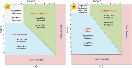
Figure 3(b) represents the structure of the optimal production, rationing, and routing policies in a network with two heterogeneous participating manufacturers. For a cooperative network with heterogeneous manufacturers, the optimal threshold levels for production, rationing, and routing policies are different for the participating manufacturers based on their own parameters. In this case, the optimal rationing level for the first producer is smaller than the second producer because the second one sells the products to his own customers with a higher price. Our numerical results show that the optimal routing policy for the network with heterogeneous producers does not follow any specific rule such as variants of JSQ and it completely depends on the parameters of the whole system.

6. Approximate analysis of a dynamic network with a high number of homogeneous producers

When all the producers are homogeneous, the performance of a dynamic cooperative network with high number of producers can be evaluated approximately by using the observations on the structure of the optimal production, rationing, and routing policies discussed in Section 5.2.

Based on our discussion in Section 5.2, for the network with identical participants, the optimal routing policy is defined by JSQ. It means that the producer with the highest number of finished items over the rationing level will receive the arriving external request. When a large number of identical manufacturers cooperate in the network, the inventory levels are expected to change in a very similar pattern and the probability of receiving an external customer from the network is expected to be almost the same among all the producers over the rationing value.

Based on the numerical results that confirm this intuition, we propose approximating the JSQ routing policy with a rationing level routing policy which sends an arriving external customer to one of the producers, whose on-hand inventories are above the rationing thresholds with the same probability. If there are no available producers at the time of the arrival, the order is lost. Therefore, we present an approximation method to evaluate the performance of the system that uses the rationing-based routing and threshold-based production and rationing policies. Once the policies are given, the resulting queuing network can be analysed by using the Single Queue Approximation (SQA).

6.1. Single queue approximation

The main idea behind SQA is analysing each queue in the network independently from the others and approximating the steady-state queue length probabilities by capturing the effect of other queues on each single queue through modelling the arriving process by a stochastic process with state dependent rates (Gupta et al. 2007).

In $M/M/K/R$ model, where K is the number of servers and R is any stationary queue length-dependent routing policy, SQA with the exact arrival rate yields the same steady-state queue length distribution as in original $M/M/K/R$ model. We use this result to prove that we can approximate the steady-state probabilities of inventories for each producer in the network by defining the state-dependent arrival rates appropriately.

Proposition 6.1

The cooperative network with N participant manufacturers under the time-stationary, rationing level-based routing policy can be modelled as a $M/M/N/R$ queue where R is the rationing level routing policy of the network. Therefore, the single queue approximation with the exact state-dependent arrival rates leads to the same steady-state queue length distribution as in the original $M/M/N/R$ model for the cooperative network model.

The proof is given in the Appendix.

Therefore, in the case of cooperation, we can write the profit maximisation problem for a single producer as given below. The subscription i is omitted in the formulation because the parameters are the same for all members. (23) $\begin{array}{rl}& {\mathrm{\Pi }}_c^{\ast }=\underset{S_c,R_c}{\max }{\mathrm{\Pi }}_c\\ & \text{subject to:}{\gamma }_c\ge \gamma .\end{array}$(23) where (24) ${\mathrm{\Pi }}_c=\lambda \left(Pr\right(I_c>0\left)\right)p+{\lambda }_a\left(Pr\right(I_c>R_c\left)\right)p_e-h{\overline{I}}_c.$(24) and (25) $\begin{array}{rl}{\gamma }_c& =1-Pr(I_{c_1}\le R_{c_1},I_{c_2}\le R_{c_2},\dots ,I_{c_N}\le R_{c_N}).\end{array}$(25) (26) $\begin{array}{rl}& {\gamma }_c\approx 1-[1-Pr(I_c>R_c){]}^N.\end{array}$(26) Note that the exact state-dependent arrival rate of external customers for a single producer in the network is defined by ${\lambda }_a$ in Equation (24(24) ${\mathrm{\Pi }}_c=\lambda \left(Pr\right(I_c>0\left)\right)p+{\lambda }_a\left(Pr\right(I_c>R_c\left)\right)p_e-h{\overline{I}}_c.$(24) ). Similar to the previous cases, the producers will decide to enter the cooperative network-based on the expected profit rates. We define the decision of joining the cooperative network with the rationing-based routing policy (cr) or operating independently (nc) by $g_{r_i}\in \{cr,nc\}$. The optimal decision $g_{r_i}^{\ast }$ is determined as: (27) $g_{r_i}^{\ast }=\left\{\begin{array}{ll}cr\left(cooperation\right)& \mathrm{if}{\mathrm{\Pi }}_c^{\ast }=max\{{\mathrm{\Pi }}_c^{\ast },{\mathrm{\Pi }}_{nc}^{\ast }\}\\ nc\left(nocooperation\right)& \mathrm{if}{\mathrm{\Pi }}_{nc}^{\ast }=max\{{\mathrm{\Pi }}_c^{\ast },{\mathrm{\Pi }}_{nc}^{\ast }\}\end{array}\right..$(27)

6.2. Approximate analysis of the cooperative network

Based on Proposition 6.1, the single queue approximation yields a significant computational efficiency for analysing the cooperative production network with N producers if a good approximation for state-dependent arrival rate can be determined. In this part, we will derive a closed-form approximation for the single queue arrival rate denoted with ${\lambda }_a$.

Let us assume that when an external customer is routed to one of the producers since its inventory level is greater than the rationing value, there are J producers which also have inventory levels greater than $R_c$ among the other N−1 members of the network. Since it is equally likely for all the available producers to receive the arriving second-class customer, the approximate long-run rate for receiving external customers ${\lambda }_a$ is (28) ${\lambda }_a\approx {\lambda }_e\left(\sum _{j=0}^{N-1}\frac{1}{j+1}Pr(J=j)\right)$(28) where J is a random variable that shows the number of available producers at the time of arrival. Since the steady-state probability of satisfying external demand for a producer is $Pr(I_c>R_c)$, $Pr(J=j)$ can be approximated by using the binomial distribution: (29) $Pr(J=j)\approx \left(\begin{array}{c}N-1\\ j\end{array}\right)\left(Pr\right(I_c>R_c\left){)}^j\right(1-Pr(I_c>R_c){)}^{N-j-1}.$(29) Equations (28(28) ${\lambda }_a\approx {\lambda }_e\left(\sum _{j=0}^{N-1}\frac{1}{j+1}Pr(J=j)\right)$(28) ) and Equation (29(29) $Pr(J=j)\approx \left(\begin{array}{c}N-1\\ j\end{array}\right)\left(Pr\right(I_c>R_c\left){)}^j\right(1-Pr(I_c>R_c){)}^{N-j-1}.$(29) ) yield the following closed-form approximation for ${\lambda }_a$: (30) ${\lambda }_a\approx {\lambda }_e\frac{1-(1-Pr(I_c>R_c){)}^N}{NPr(I_c>R_c)}.$(30) The network will accept the external customers, if it can offer this group of customers the predetermined service level (γ) and we have: (31) ${\lambda }_a\approx \left\{\begin{array}{ll}{\lambda }_e\frac{1-(1-Pr(I_c>R_c){)}^N}{NPr(I_c>R_c)}& \mathrm{if}{\gamma }_c\ge \gamma \\ 0& \mathrm{if}{\gamma }_c<\gamma \end{array}\right..$(31) When the inter-arrival time distribution of external customers is approximated with an exponential distribution with the rate ${\lambda }_a$, the resulting model is the same as the make-to-stock M/M/1 queue with two classes of customers that was used in Section 4. Accordingly, Equation (2(2) $\begin{array}{rl}Pr(I_{{nc}_i}>R_{{nc}_i})& =1-\frac{(1-{\xi }_{{nc}_i}){\xi }_{{nc}_i}^{S_{{nc}_i}-R_{{nc}_i}}(1-{\rho }_i^{R_{{nc}_i}+1})}{(1-{\rho }_i)(1-{\xi }_{{nc}_i}^{S_{{nc}_i}-R_{{nc}_i}})+(1-{\xi }_{{nc}_i}){\xi }_{{nc}_i}^{S_{{nc}_i}-R_{{nc}_i}}(1-{\rho }_i^{R_{{nc}_i}+1})},\end{array}$(2) ) yields $Pr(I_c>R_c)$ for a given value of ${\xi }_c=(\lambda +{\lambda }_a)/\mu$. Since ${\lambda }_a$ is approximated by using the expression for a given $Pr(I_c>R_c)$ in Equation (30(30) ${\lambda }_a\approx {\lambda }_e\frac{1-(1-Pr(I_c>R_c){)}^N}{NPr(I_c>R_c)}.$(30) ), combining these two equalities yields a non-linear equality for $Pr(I_c>R_c)$. For given values of $S_c$ and $R_c$, this non-linear equation is solved first to determine $Pr(I_c>R_c)$. This solution yields the corresponding ${\xi }_c$ that is used to determine $Pr(I_c>0)$ and ${\overline{I}}_c$ respectively.

6.3. Accuracy of the approximation method

In order to evaluate the accuracy of single queue approximation method, we model a cooperative network with 2, 4, 6, 8, 10 members where each member uses one of the six pairs of base-stock levels (up to 15) and rationing levels up (up to 12). For the cases where N=2,4, the exact solution is determined by using the state-space model. For the cases N=6,8,10, estimates for the exact solution are obtained by simulation where the simulation length is set to get results with the same number of significant digits as the approximation method. Comparison of the results show that the average errors for $Pr(I_c>0)$, $Pr(I_c>R_c)$, ${\overline{I}}_c$, ${\lambda }_a$ and ${\gamma }_c$ are $0.5\mathrm{\%},2.7\mathrm{\%},3.9\mathrm{\%},0.02\mathrm{\%},0.03\mathrm{\%}$ respectively.

Figure 4. The percentage error of profit between the exact solution of dynamic network and its approximation using the single queue method (Group 1:$\lambda =3,{\lambda }_{ei}=4,p=100,p_e=50,h=15,\mu =5,\gamma =0.65$, Group 2:$\lambda =4,{\lambda }_{ei}=6,p=100,p_e=50,h=15,\mu =7,\gamma =0.75$, Group 3:$\lambda =5,{\lambda }_{ei}=4,p=100,p_e=70,h=15,\mu =6,\gamma =0.8$)

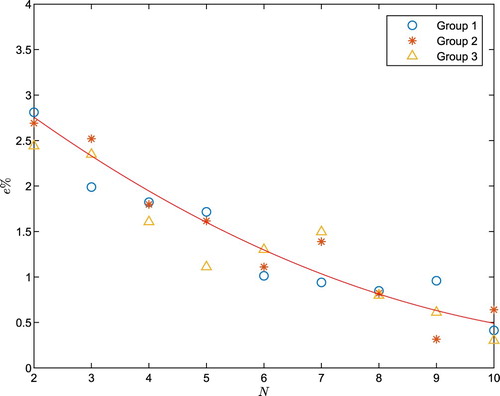
Figure 4 shows the percentage of error ($e\mathrm{\%}$) between the value of obtained profit in Equation (11(11) ${\mathrm{\Pi }}_{cd}=\sum _x\sum _u\sum _f\sum _d{\mathrm{\Pi }}_{xfd}{P}_{xufd}$(11) ) and the resulting value from the single queue approximation in Equation (24(24) ${\mathrm{\Pi }}_c=\lambda \left(Pr\right(I_c>0\left)\right)p+{\lambda }_a\left(Pr\right(I_c>R_c\left)\right)p_e-h{\overline{I}}_c.$(24) ) in 30 different cases. Each group of points gives the error values of profit for a specific network with different number of identical participants (N). We apply the best fit for these values of percentage error in Figure 4. This figure shows that the maximum error is 2.7% when there are two cooperating producers and decreases below 1% when there are more than seven producers. These results show that the single queue approximation is quite accurate and therefore can be used to evaluate the performance of the operation of a cooperative production network.

6.4. Operation of the cooperative production network for a large number of homogeneous producers

The main advantage of a cooperative network is increasing the profit for all participants. By entering the network, all manufacturers receive the demand from the external customers at a higher rate. The increased external demand leads to a higher profit compared to the case where they operate independently. Our next result shows that the cooperative network with identical producers yields a profit that is greater than or equal to the profit obtained in the independent operation case.

Proposition 6.2

The profit obtained by each producer in the cooperative network with N homogeneous participants and a rationing level routing policy is always greater than or equal to the profit obtained in the independent setting where the producers operate independently.

The proof is given in the Appendix.

Given the system parameters and the production and sales policies variables, the approach described in the preceding section yields the expected profit for each producer in both settings. When the network operates with its members optimising their own objectives, each producer maximises his own profit rate function to determine the optimal values of the base-stock level $S_c^{\ast }$ and the rationing level $R_c^{\ast }$ for given values of the price $p_e$ and the arrival rate of the external customers ${\lambda }_a$ given by the network. This is referred as the localised operation of the network.

The localised operation of the cooperative production network gives the same total profit as the global operation of the network where all the base stock and rationing levels are defined centrally by the network.

7. Benefit of joining a cooperative network

In this section, we discuss the financial and service level benefits of the cooperative networks through a set of numerical experiments. To this end, we focus on a range of offered price and desired service level for the external business offer (${\lambda }_{ei}$, $p_{ei}$, γ) and discuss how the region to accept these offers is enlarged as a result of cooperation among producers.

First, we will discuss the performance of the cooperative network when the members are homogeneous. Then we will continue our discussion for the networks with heterogeneous participants. In the last part of numerical experiments, we use the approximate analytical model derived in Section 6 to see the benefits of cooperation among a large number of homogeneous manufacturers.

7.1. Performance of the dynamic cooperative networks with homogeneous members

Figure 5 shows the decisions to accept or reject the external business offer $({\lambda }_e,p_e,\gamma )$ for the independent operation and the cooperative network with two identical members. As it was mentioned before in Section 4, in the boundary graphs, the external business offer is accepted for the set of prices and requested service levels in all of the points under the boundary line. However, this offer is rejected in all combinations of prices and desired service levels over the boundary line. Making a comparison between the independent operation in Figure 5(a) and cooperative network in Figure 5(b) shows that the network improves the accepting area significantly and it is very effective for accepting the external offers with high required service levels even with just two homogeneous members.

Figure 5. (a) The boundary between the external customers' accept and reject regions for different values of selling price $p_e$ and requested service level γ in independent operation ($\lambda =3,\mu =5,{\lambda }_{e1}=4,p_1=100,h=5$), (b) The boundary between the external customers' accept and reject regions for different values of selling price $p_e$ and requested service level γ in dynamic network with two identical members (${\lambda }_1={\lambda }_2=3,{\mu }_1={\mu }_2=5,{\lambda }_{e1}={\lambda }_{e2}=4,p_1=p_2=100,h_1=h_2=5$).

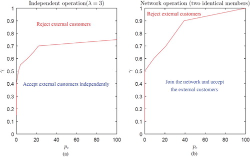
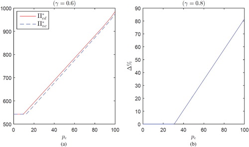
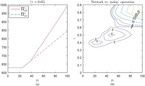
Figure 6 shows some results about the total profit comparing the independent operation and dynamic cooperative network in two different occasions. In Figure 6(a), the desired service level is $\gamma =0.6$ and the producers are capable of accepting external customers independently. Entering to the cooperative network with homogeneous participants would not improve the profit of members significantly in this case. However, in Figure 6(b), the desired service level is $\gamma =0.8$ which make it impossible to accept external offers independently for the producers. Joining the cooperative network in this case, enables the participants to enjoy the external business offer by utilising their capacity more effectively and making more profit. According to Figure 6, we can observe up to $80\mathrm{\%}$ profit increase between the independent operation and the cooperative network depending on the value of $p_e$ when $\gamma =0.8$.

Figure 6. (a) Profit rate change in response to different values of selling price $p_e$ and specified (γ) in a cooperative network with two identical members when $\gamma =0.6$, (b) Percentage of profit increase in response to different values of selling price $p_e$ and specified (γ) in a cooperative network with two identical members when $\gamma =0.8$, (${\lambda }_1={\lambda }_2=3,{\mu }_1={\mu }_2=5,{\lambda }_{e1}={\lambda }_{e2}=4,p_1=p_2=100,h_1=h_2=5$).

7.2. Performance of the Dynamic Cooperative Networks with Heterogeneous Members

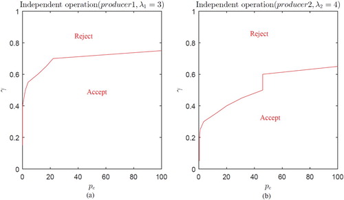
In order to analyse the behaviour of the cooperative network with heterogeneous members, we consider two manufacturers with different utilisations as shown in Figure 7. Making a comparison between Figure 7(a) and 7(b), we can see that the region of accepting external business offers is much smaller for the second producer that receives his own customers with higher rate (higher utilisation).

Figure 7. (a) The boundary between the external offers' accept and reject regions for different values of selling price $p_e$ and requested service level (γ) in independent operation when ${\lambda }_1=3$, (b) The boundary between the external offers' accept and reject regions for different values of selling price $p_e$ and requested service level (γ) in independent operation when ${\lambda }_2=4$, (${\mu }_1={\mu }_2=5,{\lambda }_{e1}={\lambda }_{e2}=4,p_1=p_2=100,h_1=h_2=5$).

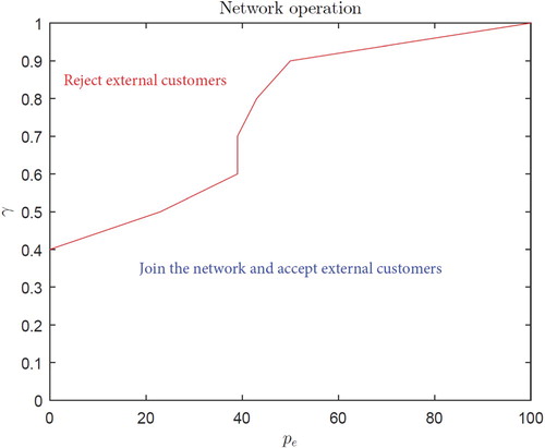
A cooperative network is formed by these two producers in the areas that both manufacturers decide to join the network. Figure 8 shows the boundaries of these regions for the dynamic cooperative network. Comparing the areas with independent operations in Figure 7 shows that the dynamic network enlarges the region to accept external business offers and enables the system to accept the offers even with high values of the desired service level.

Figure 8. The boundary between the external offers' accept and reject regions for different values of selling price $p_e$ and requested service level γ in dynamic network with two heterogeneous members (${\mu }_1={\mu }_2=5,{\lambda }_{e1}={\lambda }_{e2}=4,p_1=p_2=100,h_1=h_2=5$).

The good performance of the cooperative network is the result of dynamic routing policy and its sensitivity to the inventory levels at any time. Because of this reason, in a network with heterogeneous members where the inventory levels behave in a very different way, dynamic network performs effectively and we observe a more significant profit improvement in a dynamic cooperative network with heterogeneous members compared to the network with homogeneous participants. Figure 9(a) presents the profit rates for the independent operation and the cooperative dynamic network. According to this figure, even for the required service level $\gamma =0.65$ that the producers could accept external offers independently, we can observe up to $15\mathrm{\%}$ increase in the profit by joining the cooperative network.

Figure 9. (a) The profit for different values of selling price $p_e$ and requested service level ($\gamma =0.65$) in independent operation and dynamic network with two heterogeneous members, (b) The percentage of profit increase ($\mathrm{\Delta \%}$) for different values of selling price $p_e$ and requested service level γ in a network with dynamic routing policy and two heterogeneous members, (${\lambda }_1=3,{\lambda }_2=4,{\mu }_1={\mu }_2=5,{\lambda }_{e1}={\lambda }_{e2}=4,p_1=p_2=100,h_1=h_2=5$).

More generally, Figure 9(b) presents the percentage of profit increase between the cooperative network and the independent operation. Accordingly, for the higher desired service levels, profit improvement is more significant.

7.3. Benefits of a cooperative network with a large number of homogeneous participants

In this section, we use the approximation method presented in Section 6 to evaluate the benefits of a cooperative network with a large number of identical participants.

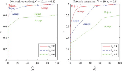
Figure 10 shows the decisions to accept or reject the external customers' business offer $({\lambda }_e,p_e,\gamma )$ in the cooperative network with 10 members. Figure 10(a,b) is given for different values of external customers arrival rate ${\lambda }_e$ and different utilisation of the participating producers (ρ). Based on these results and focusing on the acceptance area in these two settings and corresponding independent operations in Figure 2, we can see that the network will accept a larger portion of the business offers from external customers with lower prices and higher service levels. As a result, the network improves the profit compared to the independent operation, this improvement is significant for the producers with higher utilisation, that are not able to provide the high values of the desired service level for the external customers.

Figure 10. (a) External customers acceptance and rejection areas for network-based operations when $\rho =0.4$, (b)External customers acceptance and rejection areas for network-based operations when $\rho =0.8$, ($\mu =5,p=100,h=5,N=10$).

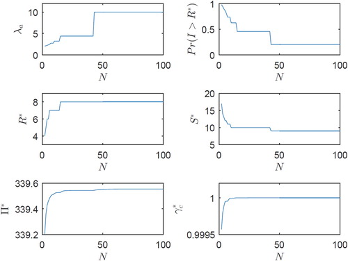
Increasing the number of participating manufacturers $\left(N\right)$ in the cooperative network, the system will behave in different ways based on its parameters. Figure 11 shows the optimal behaviour of the system for different values of $N=2,\dots ,100$ when ${\rho }_i=0.4$ and ${\lambda }_{ei}=2$. The desired service level for external customers is equal to 0.8. In this case, the producers can accept external business offer and satisfy the requested service level independently. Entering to the network gives the producers an opportunity to decrease their individually offered service level for external customers $\left(Pr\right(I_c>R_c\left)\right)$, while the network offers them their desired service level ${\gamma }_c\ge \gamma$. According to Figure 11, increasing the number of participants, the producers can decrease the value of $\left(Pr\right(I_c>R_c\left)\right)$ down to the constant value 0.2. As the result, the profit for the members will increase and the offered service level for external customers approaches to 1. Thus, it is more efficient to accept external business offers with high values of the desired service level when there is a large number of members in the network under these circumstances.

Figure 11. Optimal behaviour of the system for different number of members in the network ($\lambda =2,{\lambda }_{e_i}=2,\mu =5,p=100,p_e=70,h=0.05,\gamma =0.8$).

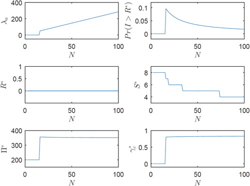
However, it may be not true for some kinds of occasions where the producers could not satisfy external business offer independently due to service level constraint. Figure 12 shows the optimal behaviour of the same system for different values of $N=2,\dots ,100$ where ${\lambda }_{ei}=6$. According to this figure, up to N=15, the network is not able to provide requested service level and rejects external business offer. From N=16, the service level constraint is satisfied and the network accepts external customers. By increasing the number of participating members in the network to the larger values, the value of $\left(Pr\right(I_c>R_c\left)\right)$ approaches to zero in this situation. Due to this reason, the value of ${\gamma }_c$ goes to a limited value less than 1 and the profit does not increase for a larger number of participants. Therefore, the number of participants in this kind of networks should be defined as the minimum number which is essential to satisfy service level constraint.

Figure 12. Optimal behaviour of the system for different number of members in the network ($\lambda =2,{\lambda }_{e_i}=6,\mu =5,p=100,p_e=70,h=0.05,\gamma =0.8$).

When the price of the external customers, $p_e$ becomes lower compared to the price obtained from the producers' own customers, the producers allocate a smaller part of their inventory for the external demand. However, having a large number of participants in the system enables the network to offer a high service level for the external customers. Figure 13(a,b) shows the service level benefit of a cooperative network with 10 members compared to the independent operation clearly. These graphs show that for the same price, the network can offer a higher service level to the external customers compared to the service level that producers offer to this group of customers independently.

Figure 13. (a) Network-based service level and independent producer-based service level for different values of price when $\rho =0.4$ and $\gamma =0.75$, (b) Network-based service level and independent producer-based service level for different values of price when $\rho =0.8$ and $\gamma =0.55$, ($\mu =5,{\lambda }_{e_i}=4,p=100,h=5$).

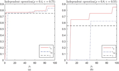
Figure 14(a) shows that the percentage increase in the profit ($\mathrm{\Delta \%}$) for producers participating in a cooperative network with 10 participants decreases with the price ratio $p/p_e$. If the price obtained from the producers' own customers is much higher than the price obtained from the external customers, the producer prefers to serve his own customers and the system gets closer to the one with a single demand class. Hence, the network does not yield more benefit. Figure 14(b) shows the percentage increase in the profit ($\mathrm{\Delta \%}$) for different values of $p_e$ when p is equal to 100. This result also shows that entering the cooperative network is more beneficial for producers as the price for the external customers increases and gets closer to the price obtained from their own customers, p.

Figure 14. (a) Percentage of profit increase for cooperative network compared to independent operation for different values of price ratio $p/p_e$ (b) Percentage of profit increase for cooperative network compared to independent operation for different values of price $p_e$ ($\lambda =4,\mu =5,{\lambda }_e=20,p=100,h=5,\gamma =0.85,N=10$).

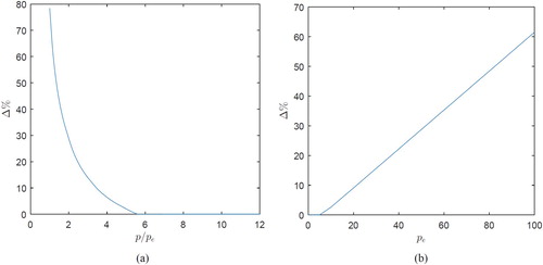
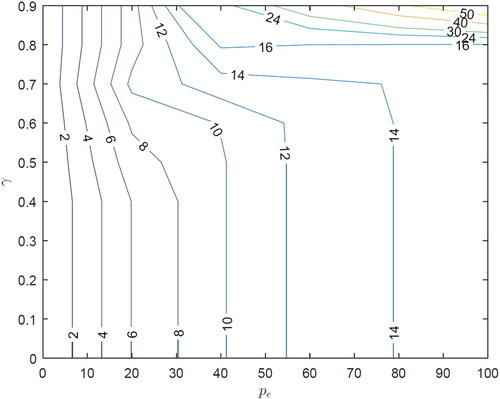
Figure 15 also shows the percentage profit increase ($\mathrm{\Delta \%}$) for different values of price ($p_e$) and the requested service level (γ). According to this graph, for the lower levels of the requested service level, the profit increase as a result of joining the network is limited. As the requested service level increases, the independent producers start rejecting the external business offers for the lower values of $p_e$. On the other hand, the network continues accepting these offers even for lower prices. This fact leads to a larger percentage of profit increase for higher requested service levels.

Figure 15. Profit increase $\mathrm{\Delta \%}$ for different values of price $p_e$ and requested service level γ ($\lambda =4,\mu =5,{\lambda }_{ei}=2,p=100,h=5,N=10$).

8. A summary of findings

In this section, we summarise our findings that may provide insights. We group our findings for cooperative networks among homogeneous producers and cooperation among heterogeneous producers.

When homogeneous manufacturers consider cooperation,

• if it is optimal for them to accept the external offers when they operate independently, it is always beneficial to join the cooperative network;

• the cooperative network will be more beneficial when the price for the external customers gets closer to the price received from the producers' own customers;

• cooperation in a network that uses a dynamic routing policy with the on-line inventory information of the network members brings significant benefits especially when the requested service level is high.

When heterogeneous manufacturers with different parameters consider cooperation,

• in order to have a successful cooperative network, each partner should contribute either by its higher external demand rate, higher production capacity or more profitable external sales;

• if a producer dominates others in all these features, cooperation between these producers can decrease the overall total profit;

• using a dynamic routing policy that utilises the on-line inventory information in a cooperative network leads to a higher improvement for a network with heterogeneous members compared to a network with homogeneous members, since the dynamic routing policy can react to changes in the inventory levels of heterogeneous producers effectively.

9. Concluding remarks

In this paper, we present an analytical model of a cooperative network among a number of manufacturers that want to increase their utilisation and profit as a result of this cooperation. Our analysis is performed on the cooperative network with dynamic routing policy and we determine the optimal production, rationing and routing policies using mathematical programming to solve the resulting Markov decision problem.

As the main contribution of this study, we examined the detailed operational model of cooperation in a network and analysed the optimal production, rationing, and routing decisions jointly in our model.

Our results show that a dynamic cooperative network yields a significant financial and service level improvement compared to the independent operation. We also show that for a dynamic network with identical members, the optimal routing policy follows the JSQ rule and the level of inventories are changing in a very similar way to each other, based on this observation. As the result, we suggest an approximation analysis of this kind of network with a lower computational effort. We prove that we can approximate this structure just by analysing a single queue in the network by using the single queue approximation. Using this procedure, we found the steady-state probabilities of queue length to analyse the system performance. Our results show the high accuracy of our approximation method compared to analytical results.

The results that are based on the analytical model show that a cooperative production network increases the producers profit especially when the external customers require a high service level. In addition, the main benefit of a cooperative production network is its ability to provide a significantly higher service level to customers compared to the service level these customers would get from the producers independently.

In the case of mass cooperation, such as the case in cloud manufacturing, the network can provide close to $100\mathrm{\%}$ service level and accept external customers even when they offer a very low price. As a result, the possibility of offering a high service level and low price will give a competitive advantage to the members of the cooperative network.

Our model can be extended to examine the optimal coalition structure in the network. The optimal coalition scheme between the participating producers may involve multiple interoperable networks to maximise the total profit while ensuring that each producer is better off compared to the independent operation. Similarly, the competition among participating producers can be analysed by using game theoretical approaches. The model can also be extended to derive optimal rationing policies for different customer classes with different service level expectations. These are left for future research.

As another direction of this research, we can focus on modelling and analysis of a cooperative service network. One of the practical examples for this kind of service networks is telemedicine platforms that use telecommunication to provide health care services, such as health consultations. It is very important to manage this network effectively to offer the patients more specialised and faster service with lower costs.

Disclosure statement

No potential conflict of interest was reported by the authors.

ORCID

Barış Tan  http://orcid.org/0000-0002-2584-1020

Additional information

Funding

Research leading to these results has received funding from the EU ECSEL Joint Undertaking under grant agreement no. 737459 (project Productive4.0) and from TUBITAK (217M145).

Appendices

A.1. Proof of Proposition 6.1

The proof is similar to the one which is used in Gupta et al. (2007). We consider the case where there are two producers $(N=2)$. The result for N>2 is a straightforward expansion of this result and it is not given here.

Based on our assumptions about the system, the system is modelled as a continuous time Markov chain where the state of the system is a two-dimensional vector representing the number of items at each inventory. Let ${\pi }_{n+1,j}$ be the steady-state probability when there are n+1 items in the first inventory and j items in the second one. The steady-state probability of having n items in the first inventory, $P_n$, can be written as follows: (A1) $P_{n+1}=\sum _{j=0}^S{\pi }_{n+1,j}.$(A1)

The customer arrival rate to the first producer that is the arrival rate of customers depending on the number of items in the inventory (${\lambda }_{n+1}$) can be defined as: (A2) ${\lambda }_{(n+1)}=\sum _{j=0}^S\left({\pi }_{n+1,j}/P_{n+1}\right)({\lambda }_1+{\lambda }_e{q}_{(n+1,j)})$(A2) where $q_{n+1,j}$ is the probability that the router routes a demand to the first inventory when there are n+1 items in the first inventory and j items in the second inventory. For two participants, we have: (A3) $q_{(n+1,j)}=\left\{\begin{array}{ll}1/2& \mathrm{if}n+1>R,j>R\\ 1& \mathrm{if}n+1>R,j\le R\\ 0& \mathrm{if}n+1<R\end{array}\right.$(A3)

Writing the balance equations between the set of states $T_n=\left\{\right(n,j):j=0,\dots ,S\}$ and $T_{n+1}=\left\{\right(n+1,j):j=0,\dots ,S\}$, we have: (A4) $\sum _{j=0}^S{\pi }_{n,j}\mu =\sum _{j=0}^S{\pi }_{n+1,j}({\lambda }_1+{\lambda }_e{q}_{(n+1,j)}).$(A4)

Following Equation (A2(A2) ${\lambda }_{(n+1)}=\sum _{j=0}^S\left({\pi }_{n+1,j}/P_{n+1}\right)({\lambda }_1+{\lambda }_e{q}_{(n+1,j)})$(A2) ), we can write (A5) $P_{n+1}{\lambda }_{(n+1)}=\sum _{j=0}^S{\pi }_{n+1,j}({\lambda }_1+{\lambda }_e{q}_{(n+1,j)}).$(A5)

Therefore, from (A4(A4) $\sum _{j=0}^S{\pi }_{n,j}\mu =\sum _{j=0}^S{\pi }_{n+1,j}({\lambda }_1+{\lambda }_e{q}_{(n+1,j)}).$(A4) ) and (A5(A5) $P_{n+1}{\lambda }_{(n+1)}=\sum _{j=0}^S{\pi }_{n+1,j}({\lambda }_1+{\lambda }_e{q}_{(n+1,j)}).$(A5) ), we have the following result: (A6) $P_{n+1}{\lambda }_{(n+1)}=P_n\mu$(A6)

On the other hand, using SQA we can model the network as $M_n/M/1$ which is a queue with conditional arrival rate $\lambda \left(n\right)$ and the steady-state probability of having n items in the inventory $x_n$. So, writing the balance equation for this model will result in the following equation: (A7) $x_{n+1}{\lambda }_{(n+1)}=x_n\mu .$(A7)

Comparing Equations (A6(A6) $P_{n+1}{\lambda }_{(n+1)}=P_n\mu$(A6) ) and (A7(A7) $x_{n+1}{\lambda }_{(n+1)}=x_n\mu .$(A7) ) yield (A8) $x_n=P_n.$(A8)

Namely, with the exact state-dependent arrival rates (${\lambda }_n$), the single queue approximation yields the same steady-state queue length distribution as in the original model of network. $◻$

A.2. Proof of Proposition 6.2

Based on the approximated value of ${\lambda }_N$ in Equation (30(30) ${\lambda }_a\approx {\lambda }_e\frac{1-(1-Pr(I_c>R_c){)}^N}{NPr(I_c>R_c)}.$(30) ), we can say that: (A9) $\frac{(1-(1-Pr(I_c>R_c){)}^N)}{Pr(I_c>R_c)}\ge 1.$(A9)

Therefore: (10) $\left({\lambda }_e/N\right)\frac{(1-(1-Pr(I_c>R_c){)}^N)}{Pr(I_c>R_c)}\ge \left({\lambda }_e/N\right).$(10)

This means that in the network-based setting with the $Pr(I_c>R_c)$ less than one, all producers will receive the second-class customers with a higher rate in comparison to independent case. Decreasing the value of price $p_e$, the participants will try to allocate smaller part of their inventory for second-class demand, therefore the value of this probability will decrease and the difference between second-class customers arrival rates in two cases becomes larger.

Therefore, using single queue approximation, we have two settings which differ in the rate of second-class customers' arrival. The first one is the independent setting with the profit function ${\pi }_{nc}({\lambda }_1,({\lambda }_e/N),S_{nc}^{\ast },R_{nc}^{\ast })$ and the second one is the cooperative case with the profit function ${\pi }_c({\lambda }_1,({\lambda }_e/N)+\mathrm{\Delta },S_c^{\ast },R_c^{\ast })$ with $0\le \mathrm{\Delta }$.

Assuming that in the cooperative setting, we apply a control policy which filters the second-class customers and reduce the rate of arrival for second group of customers to $\left({\lambda }_e/N\right)$ and then use $S_{nc}^{\ast }$ and $R_{nc}^{\ast }$ as production and selling policies, we have: (A11) ${\pi }_c({\lambda }_1,({\lambda }_e/N)+\mathrm{\Delta },S_{nc}^{\ast },R_{nc}^{\ast })={\pi }_{nc}^{\ast }({\lambda }_1,({\lambda }_e/N),S_{nc}^{\ast },R_{nc}^{\ast }).$(A11)

Also, we know that: (A12) $\{R_c^{\ast },S_c^{\ast }\}=\underset{}{\mathrm{argmax}}\left\{{\pi }_c\right({\lambda }_1,\left({\lambda }_e/N\right)+\mathrm{\Delta },S_c,R_c\left)\right\}.$(A12)

Therefore: (A13) ${\pi }_c^{\ast }({\lambda }_1,({\lambda }_e/N)+\mathrm{\Delta },R_c^{\ast },S_c^{\ast })\ge {\pi }_c({\lambda }_1,({\lambda }_e/N)+\mathrm{\Delta },S_c,R_c).$(A13)

Comparing Equations (A11(A11) ${\pi }_c({\lambda }_1,({\lambda }_e/N)+\mathrm{\Delta },S_{nc}^{\ast },R_{nc}^{\ast })={\pi }_{nc}^{\ast }({\lambda }_1,({\lambda }_e/N),S_{nc}^{\ast },R_{nc}^{\ast }).$(A11) ) and (A13(A13) ${\pi }_c^{\ast }({\lambda }_1,({\lambda }_e/N)+\mathrm{\Delta },R_c^{\ast },S_c^{\ast })\ge {\pi }_c({\lambda }_1,({\lambda }_e/N)+\mathrm{\Delta },S_c,R_c).$(A13) ), we have: (A14) ${\pi }_c^{\ast }({\lambda }_1,({\lambda }_e/N)+\mathrm{\Delta },R_c^{\ast },S_c^{\ast })\ge {\pi }_{nc}^{\ast }({\lambda }_1,({\lambda }_e/N),R_{nc}^{\ast },S_{nc}^{\ast }).$(A14) $◻$

References

- Akçay, Y., and B. Tan. 2008. “On the Benefits of Assortment-based Cooperation Among Independent Producers.” Production and Operations Management 17 (6): 626–640.
- Benjaafar, S., W. L. Cooper, and J.-S. Kim. 2005. “On the Benefits of Pooling in Production-inventory Systems.” Management Science 51 (4): 548–565.
- Benjaafar, S., M. ElHafsi, and F. d. Véricourt. 2004. “Demand Allocation in Multiple-product, Multiple-facility, Make-to-stock Systems.” Management Science 50 (10): 1431–1448.
- Benjaafar, S., Y. Li, D. Xu, and S. Elhedhli. 2008. “Demand Allocation in Systems with Multiple Inventory Locations and Multiple Demand Sources.” Manufacturing & Service Operations Management 10 (1): 43–60.
- Bertsekas, D. P., D. P. Bertsekas, D. P. Bertsekas, and D. P. Bertsekas. 1995. Dynamic Programming and Optimal Control, Volume 1. Belmont, MA: Athena Scientific.
- Bhandari, A., A. Scheller-Wolf, and M. Harchol-Balter. 2008. “An Exact and Efficient Algorithm for the Constrained Dynamic Operator Staffing Problem for Call Centers.” Management Science 54 (2): 339–353.
- Bucklin, L. P., and S. Sengupta. 1993. “Organizing Successful Co-marketing Alliances.” The Journal of Marketing 57 (2): 32–46.
- Carr, S., and I. Duenyas. 2000. “Optimal Admission Control and Sequencing in a Make-to-stock/make-to-order Production System.” Operations Research 48 (5): 709–720.
- Çil, E. B., E. L. Örmeci, and F. Karaesmen. 2009. “Effects of System Parameters on the Optimal Policy Structure in a Class of Queueing Control Problems.” Queueing Systems 61 (4): 273–304.
- Cohen, M. A., P. R. Kleindorfer, and H. L. Lee. 1988. “Service Constrained (s, S) Inventory Systems with Priority Demand Classes and Lost Sales.” Management Science 34 (4): 482–499.
- Danilovic, M., and M. Winroth. 2005. “A Tentative Framework for Analyzing Integration in Collaborative Manufacturing Network Settings: A Case Study.” Journal of Engineering and Technology Management22 (1): 141–158.
- Deshpande, V., M. A. Cohen, and K. Donohue. 2003. “A Threshold Inventory Rationing Policy for Service-differentiated Demand Classes.” Management Science 49 (6): 683–703.
- Duran, S., T. Liu, D. Simchi-Levi, and J. L. Swann. 2007. “Optimal Production and Inventory Policies of Priority and Price-differentiated Customers.” IIE Transactions 39 (9): 845–861.
- Ferreira, J., F. Gigante, J. Sarraipa, M. J. Nunez, C. Agostinho, and R. Jardim-Goncalves. 2014. Collaborative Production Using Dynamic Manufacturing Networks for SME's. In Engineering, Technology and Innovation (ICE), 2014 International ICE Conference on, 1–7. IEEE.
- Frank, K. C., R. Q. Zhang, and I. Duenyas. 2003. “Optimal Policies for Inventory Systems with Priority Demand Classes.” Operations Research 51 (6): 993–1002.
- Gayon, J.-P., S. Benjaafar, and F. De Véricourt. 2009. “Using Imperfect Advance Demand Information in Production-inventory Systems with Multiple Customer Classes.” Manufacturing & Service Operations Management 11 (1): 128–143.
- Gayon, J.-P., F. De Vericourt, and F. Karaesmen. 2009. “Stock Rationing in An M/Er/1 Multi-class Make-to-stock Queue with Backorders.” IIE Transactions 41 (12): 1096–1109.
- Gupta, V., M. H. Balter, K. Sigman, and W. Whitt. 2007. “Analysis of Join-the-shortest-queue Routing for Web Server Farms.” Performance Evaluation 64 (9): 1062–1081.
- Ha, A. Y.. 1997a. “Inventory Rationing in a Make-to-stock Production System with Several Demand Classes and Lost Sales.” Management Science 43 (8): 1093–1103.
- Ha, A. Y.. 1997b. “Stock-rationing Policy for a Make-to-stock Production System with Two Priority Classes and Backordering.” Naval Research Logistics 44 (5): 457–472.
- Huang, B., and S. M. Iravani. 2007. “Optimal Production and Rationing Decisions in Supply Chains with Information Sharing.” Operations Research Letters 35 (5): 669–676.
- Ivanov, D., A. Dolgui, B. Sokolov, F. Werner, and M. Ivanova. 2016. “A Dynamic Model and An Algorithm for Short-term Supply Chain Scheduling in the Smart Factory Industry 4.0.” International Journal of Production Research 54 (2): 386–402.
- Lee, J. E., and Y. Hong. 2003. “A Stock Rationing Policy in a (s, S) Controlled Stochastic Production System with 2-phase Coxian Processing Times and Lost Sales.” International Journal of Production Economics 83 (3): 299–307.
- Li, B.-H., L. Zhang, S.-L. Wang, F. Tao, J. Cao, X. Jiang, X. Song, and X. Chai. 2010. “Cloud Manufacturing: a New Service-oriented Networked Manufacturing Model.” Computer Integrated Manufacturing Systems 16 (1): 1–7.
- Liu, S., M. Song, K. C. Tan, and C. Zhang. 2015. “Multi-class Dynamic Inventory Rationing with Stochastic Demands and Backordering.” European Journal of Operational Research 244 (1): 153–163.
- Nadar, E., M. Akan, and A. Scheller-Wolf. 2016. “Experimental Results Indicating Lattice-dependent Policies May Be Optimal for General Assemble-to-order Systems.” Production and Operations Management 25 (4): 647–661.
- Nahmias, S., and W. S. Demmy. 1981. “Operating Characteristics of An Inventory System with Rationing.” Management Science 27 (11): 1236–1245.
- Pang, Z., H. Shen, and T. Cheng. 2014. “Inventory Rationing in a Make-to-stock System with Batch Production and Lost Sales.” Production and Operations Management 23 (7): 1243–1257.
- Papakostas, N., K. Efthymiou, K. Georgoulias, and G. Chryssolouris. 2013. “On the Configuration and Planning of Dynamic Manufacturing Networks.” In Robust Manufacturing Control, 247–258. Berlin, Heidelberg: Springer.
- Pietrabissa, A.. 2008. “An Alternative Lp Formulation of the Admission Control Problem in Multiclass Networks.” IEEE Transactions on Automatic Control 53 (3): 839–845.
- Puterman, M. L. 2014. Markov Decision Processes: Discrete Stochastic Dynamic Programming. Inc., New York, NY: John Wiley & Sons.
- Putnik, G.. 2012. “Advanced Manufacturing Systems and Enterprises: Cloud and Ubiquitous Manufacturing and An Architecture.” Journal of Applied Engineering Science 10 (3): 127–134.
- Ren, L., L. Zhang, L. Wang, F. Tao, and X. Chai. 2014. Cloud Manufacturing: Key Characteristics and Applications. International Journal of Computer Integrated Manufacturing (Published online), 1–15.
- Swaminathan, V., and C. Moorman. 2009. “Marketing Alliances, Firm Networks, and Firm Value Creation.” Journal of Marketing 73 (5): 52–69.
- Tan, B.. 2006. “Modelling and Analysis of a Network Organization for Cooperation of Manufacturers on Production Capacity.” Mathematical Problems in Engineering 2006: 1–24.
- Tan, B., and Y. Akçay. 2014. “Assortment-based Cooperation Between Two Make-to-stock Firms.” IIE Transactions 46 (3): 213–229.
- Topkis, D. M.. 1968. “Optimal Ordering and Rationing Policies in a Nonstationary Dynamic Inventory Model with N Demand Classes.” Management Science 15 (3): 160–176.
- Véricourt, F. d., F. Karaesmen, and Y. Dallery. 2001. “Assessing the Benefits of Different Stock-allocation Policies for a Make-to-stock Production System.” Manufacturing & Service Operations Management 3 (2): 105–121.
- Véricourt, F. d., F. Karaesmen, and Y. Dallery. 2002. “Optimal Stock Allocation for a Capacitated Supply System.” Management Science 48 (11): 1486–1501.
- Wadhwa, S., M. Mishra, and F. T. Chan. 2009. “Organizing a Virtual Manufacturing Enterprise: An Analytic Network Process Based Approach for Enterprise Flexibility.” International Journal of Production Research 47 (1): 163–186.
- Wu, D., M. J. Greer, D. W. Rosen, and D. Schaefer. 2013. “Cloud Manufacturing: Strategic Vision and State-of-the-art.” Journal of Manufacturing Systems 32 (4): 564–579.
- Yu, Y., S. Benjaafar, and Y. Gerchak. 2015. “Capacity Sharing and Cost Allocation Among Independent Firms with Congestion.” Production and Operations Management 24 (8): 1285–1310.
- Zhang, L., Y. Luo, F. Tao, B. H. Li, L. Ren, X. Zhang, H. Guo, Y. Cheng, A. Hu, and Y. Liu. 2014. “Cloud Manufacturing: A New Manufacturing Paradigm.” Enterprise Information Systems 8 (2): 167–187.