Integrated decision-making in reverse logistics: an optimisation of interacting acquisition, grading and disposition processes

Abstract

In view of global environmental and social challenges the transition towards a Circular Economy is considered as a crucial factor for sustainable development. Therefore, the replacement of traditional linear business models involving product discard at the end of product life with concepts focusing on re-use of resources is essential. Reverse Logistics and Closed-loop Supply Chains are seen to be key elements of such a transition. Motivated by findings from a case study of an independent reprocessing company, we address integrated decision-making in Reverse Logistics in this paper. We present a non-linear optimisation model with interrelated processes in terms of acquisition of used products, grading for determination of product quality and reprocessing disposition. The decisions to be made concern the effort spent for active acquisition of used products and the number of reprocessed goods; both decisions are influenced by heterogeneous condition of used products. The consideration of deterministic and stochastic demand facilitates the representation of a variety of business cases. For both demand types we provide analytical insights in the form of complete strategies consisting of different scenarios which allow optimal decision-making under variable conditions. Numerical examples complement insights into the model by conducting a sensitivity analysis of relevant model parameters.

Keywords:

• reverse logistics
• decision support systems
• non-linear programming
• newsvendor
• integrated decision-making

1. Introduction and motivation

The transition towards a Circular Economy (CE) is a major goal of governmental institutions all over the world, willing to target ecological, economical and social challenges (Su et al. 2013; Stahel 2016; Geissdoerfer et al. 2017; European Commission 2018). In academia (Lewandowski 2016; Govindan and Hasanagic 2018) as well as in practice (e.g. Ellen MacArthur Foundation 2016) it is commonly accepted that Reverse Logistics (RL) and Closed-Loop Supply Chains are essential economical drivers enabling and stimulating the diffusion of CE-concepts.

Related to this, the attention paid to RL/CLSC is growing, driven by exogenous (like legislation) and endogenous factors such as increased profits. Original Equipment Manufacturers (OEMs) and other large business players have adopted methods of CE.¹ In addition to benefits for large firms, CE/RL/CLSC open opportunities for small- and medium-sized enterprises (SMEs) and social businesses – as for example 'Work Integration Social Enterprises' (WISE) –, which often act as independent reverse logistics providers (European Commission 2016; Lewandowski 2016).

The opportunities also involve risks: major challenges rising up when organisations implement processes dealing with RL/CLSC are the increasing complexity and uncertainty. Timely supply with sufficient used products, heterogeneous condition of acquired/returned used products, and demanding prediction of demand for reprocessed products are some of the factors which impact related processes (Govindan, Soleimani, and Kannan 2015). These factors lead to an enormous rise of complexity with respect to decision-making in such an integrated environment. In addition, several case studies and observations in practice emphasise that the processes within a company offering full reverse logistics service from acquisition of used products to sales of reprocessed items are highly interdependent (Brito, Dekker, and Flapper 2004; Dowlatshahi 2010; Abraham 2011; Chan, Chan, and Jain 2012; Lechner and Reimann 2015). Thus, the main reverse processes known from literature – acquisition, grading, and disposition – have to be considered in a joint approach: one example for interrelated processes is, for instance, that a rising acquisition amount also increases the probability to get more used products in good condition. Furthermore, both the acquisition of used products and the grading process directly impact the number of products available for reprocessing. Subramanian, Talbot, and Gupta (2010) report on conversation with practitioners who stress the need for integrated decision support systems, being a crucial point to act economically and sustainably (Subramanian, Talbot, and Gupta 2010).

In this work we present an integrated model including interdependent processes instead of separated sub-problems, mainly motivated by a case study presenting R.U.S.Z., a WISE with focus on reprocessing (Lechner and Reimann 2015). Some observations made in the case study pique our interest: (1) the maximum supply with used products is restricted; (2) the acquisition quantity of used products is depending on the spent effort and therefore controllable; (3) the acquired items are subject to heterogeneous quality; (4) the sales price for reprocessed items is constant; (5) the maximum demand for reprocessed products is restricted. Building on that, a joint acquisition-grading-disposition model basically dealing with decisions regarding active acquisition of and reprocessing cost for used products is developed. The processes interact with heterogeneous quality of acquired products. This builds a bridge to the other processes in order to focus on integrated decision-making and to explore main drivers and effects in a complex integrated model. This allows a thorough investigation and quantification of effects specifically occurring in the context of joint decision-making. To the best of the authors' knowledge, the joint consideration of interrelated acquisition, grading, and disposition processes has not yet been investigated in scientific literature.

The remaining work is organised as follows: in Section 2 we review related literature with respect to integrated decision-making in a RL-/CLSC-context. Next, in Section 3 a profit-maximising framework based on Galbreth and Blackburn (2006) is developed, which serves as the base model for the remaining research, extensions and numerical studies presented in this paper. Based on this model, numerical analyses are shown in Section 5. The conclusion and an outlook on future work finalises the work in Section 6.

2. Related literature

The scientific community has put increased emphasis on research concerning RL/CLSC in the last decades, what particularly becomes reasonable in consideration of the interest of practice, as indicated for instance by Wei et al. (2015) concerning motives and barriers of the remanufacturing industry in China (Wei et al. 2015). In this section we will explore scientific literature regarding the integration of main RL/CLSC-processes acquisition, grading and disposition.

One stream of literature primarily deals with disposition decisions. All discussed papers (Toktay, Wein, and Zenios 2000; Inderfurth, de Kok, and Flapper 2001; Inderfurth 2004; Bhattacharya, Guide, and Van Wassenhove 2006; Ferguson, Fleischmann, and Souza 2011; Reimann and Lechner 2012; Flapper, Gayon, and Vercraene 2012; Benedito and Corominas 2013; Giri and Glock 2017) assume a CLSC environment except for the RL approaches in Inderfurth (2004) and Polotski, Kenné, and Gharbi (2019). In none of the models, an active acquisition process is integrated; therefore, the amount of returned items cannot be controlled by acquisition cost, effort, or incentives. Additionally, potential heterogeneous quality of used products is not considered in any of the papers.

In three articles, the focus is on the link between acquisition of used products and the grading process. Galbreth and Blackburn (2006) present a model where a batch of used products with known quality distribution is acquired for remanufacturing to satisfy deterministic demand. They find that the optimal, cost-minimising acquisition quantity may exceed the demand: as the selection of acquired used products in a good condition reduces the reprocessing cost, these savings can outweigh the increased acquisition cost. The authors extend their model with different implementations of uncertain quality of the acquired used products in Galbreth and Blackburn (2010). They explore continuous and discrete quality levels combined with linear and non-linear remanufacturing cost functions. Hahler and Fleischmann (2016) determine optimal strategies for a product holder willing to sell her used product and an acquiring recommerce company in a sequential bargaining game under complete as well as incomplete information. In the examined setting, the product holder submits quality statements before sending the product, but the actual acquisition price paid to the product holder is based on the result of a grading process at the recommerce company (Hahler and Fleischmann 2016).

The link between acquisition of used products and the related disposition decisions is in the focus of a couple of approaches. Two of these articles (Guide, Teunter, and Van Wassenhove 2003; Zhou and Yu 2011) deal with the optimal pricing of acquisition of used goods and sales of reprocessed items, respectively. The structure of CLSCs with multiple players and the related coordination and competition mechanisms are in the focus of Atasu, Toktay, and Van Wassenhove (2013), Jung and Hwang (2011) and Kim and Goyal (2011). In Kaya (2010), a model with joint decision-making related to acquisition of used products, manufacturing, and remanufacturing is presented. In a two-period setting with stochastic demand and restricted availability of used products depending on first period's production quantity, Lechner and Reimann (2014) identify the optimal acquisition effort and manufacturing/remanufacturing quantities. Optimal acquisition, manufacturing, and remanufacturing quantities are determined in a multi-product model with stochastic demands in Shi, Zhang, and Sha (2011). A profit-maximisation of a non-linear model incorporating carbon emissions regulation, heterogeneous quality of returns, multiple products and uncertain demand is achieved by finding the best solution for acquisition/remanufacturing quantities and a quality threshold for remanufacturing by Yang et al. (2016). Finally, the link between supply side and demand when acquired cores can either be held or disposed of is in the focus of Wei and Tang (2015). By means of a real options approach for evaluation of the marginal value of holding acquired used cores, the authors show that under low core price the remanufacturer should collect more cores when the correlation between return and demand side is high, while under a high core price it should collect less under these circumstances (Wei and Tang 2015).

One topic which attracted attention in former articles is the potential value of grading and the related impact on the disposition decisions in a reverse system. Extensive numerical studies are provided for benchmarking a model without classification of used products with a system including high- and low quality returns (Aras, Boyaci, and Verter 2004) and the optimisation of a multi-stage, stochastic linear programme representing a capacitated production planning model with remanufacturing of returns in uncertain condition (Denizel, Ferguson, and Souza 2010). Behret and Korugan (2009) use a simulation-based approach to analyse a hybrid manufacturing/remanufacturing system with stochastic return times and both uncertain qualities and quantities of returns. The benefit of an implemented grading process on profit in a stochastic, dynamic production-planning model including remanufacturing of returns is shown by Ferguson et al. (2009). The authors also find that the number of quality categories has a great impact on the performance of the grading process. The objective of Inderfurth (2005) and Souza, Ketzenberg, and Guide (2002) is the joint optimisation of production and reprocessing decisions. Inderfurth (2005) determines the cost-minimising manufacturing – remanufacturing – disposal strategy for a CLSC in consideration of heterogeneous quality of returns. Souza, Ketzenberg, and Guide (2002) optimise a queuing network representing a production planning and control problem with several product quality classes. In addition, different dispatching heuristics under a service level constraint and the impact of an inaccurate grading process on average flow time are analysed. Further work with an implemented joint view of grading and disposition concerns potential competition between a manufacturer and a remanufacturer (Ferguson and Toktay 2006) and the impact of a finite product life-cycle on the optimal (re)manufacturing strategy (Geyer, Van Wassenhove, and Atasu 2007).

In the following, approaches integrating components of acquisition, grading and disposition are discussed. Optimal manufacturing and reprocessing strategies are in the focus of the following work. While Cai et al. (2014) optimise acquisition prices for high- and low-quality products and (re)manufacturing quantities, Hein, Spinler, and Kleindorfer (2012) use an integrated, single-period model with price-dependent supply and demand to optimise decisions of minimum acceptable quality and acquisition price for used products, the quality after reprocessing and the sales price of remanufactured items. In a single-/multi-period economic production quantity model, Saadany and Jaber (2010) show that a mixed manufacturing/remanufacturing strategy is superior to strategies considering solely new production or remanufacturing. Both works of Bakal and Akcali (2006) and Teunter and Flapper (2011) deal with the impact of uncertain yield information concerning acquired used products. A reverse supply chain including price-sensitive supply/demand and a stochastic number of reprocessable used products is considered in Bakal and Akcali (2006). Optimal acquisition and production strategies in the presence of uncertain quality of returns and deterministic/stochastic demand are determined in Teunter and Flapper (2011): in general, quality information concerning the acquired cores leads to higher profits compared with ignoring quality. Robotis, Bhattacharya, and Wassenhove (2005) show that the option to remanufacture increases the company's profitability by using an integrated model with stochastic newsvendor-like demand. Further works address optimal investments in reprocessing (Robotis, Boyaci, and Verter 2012), and the impact of active/passive acquisition processes, return quantities, reusability rates of products and components, disposal strategies and various cost configurations on the system's prices, inventory levels, disposal quantities, and profitability (Vadde, Kamarth, and Gupta 2007). A potentially error-prone grading process is assumed in Tagaras and Zikopoulos (2008) and Zikopoulos and Tagaras (2008). In the two-level supply chain with stochastic demand and yield presented in Zikopoulos and Tagaras (2008), the conditions under which inaccurate sorting before actual disassembly and reprocessing is profitable are determined. A similar setting introduced in Tagaras and Zikopoulos (2008) addresses the question whether to conduct an imperfect sorting process decentralised before transportation to the remanufacturer or centralised at the remanufacturing facility after transportation. Besides the analytical and numerical approaches shown above, some research work addresses the issue of integrated RL/CLSCs by applying System Dynamics. A complex model including product life-cycles is in the focus of Georgiadis, Vlachos, and Tagaras (2006) the effects of a product life-cycle and different product return patterns on the optimal collection and remanufacturing strategies over time is explored. Further approaches concern modelling of demand-side interactions of an OEM to test various reprocessing strategies (Lehr, Thun, and Milling 2013) or the exploration of impacts regarding the length of usage-phases and return frequencies of used products on reprocessing strategies (Poles and Cheong 2009). A complex model which integrates several aspects of a view on the total life-cycle of a product is presented in Subramanian, Talbot, and Gupta (2010). The authors consider a solely numerically solvable profit-maximising model with environmental concerns, product-design decisions, and potential best reuse of the collected products.

Beyond this, Bazan, Jaber, and Zanoni (2016) focus in a review article on inventory models for reverse logistics and provide a detailed analysis of literature considering economic order/production quantity and joint economic lot size (Bazan, Jaber, and Zanoni 2016). Decision variables to be optimised in the respective models can be related to the concerned processes with respect to acquisition, grading, and disposition. In addition, the authors introduce a modelling approach for the integration of environmental and social aspects.

The research in this paper extends the presented literature: most of the work is limited to one or two sub-processes concerning RL, but only a few articles deal with models which integrate activities related to acquisition, grading, and disposition. Particularly, in many models the acquisition of used products cannot be actively controlled but the return rate is exogenously given. Furthermore, heterogeneous quality of returned items is often not considered.

Subsuming the literature review leads to the finding that the amount of scientific work with respect to integrated RL or CLSC models is limited. In consideration of the insights from various case studies dealing with reprocessing companies, this is remarkable, as the works demonstrate the existence of individual but interrelated reverse sub-processes in practice.

3. Problem description, assumptions and modelling approach

The findings of the case study about R.U.S.Z in Lechner and Reimann (2015) guide our research and serve as assumptions for modelling. R.U.S.Z is an independent work integration social enterprise (WISE) in Vienna (Austria). R.U.S.Z offers repairing and servicing of used products, but also reprocesses acquired used products. The core products for reprocessing are white goods, i.e. washing machines. Primary source of supply for washing machines are private donors: while most of the washing machines are cost-intensively collected at the donor's home, some are brought to R.U.S.Z by the donor. Based on the result of quality inspections determining the quality condition of the used product, washing machines are accordingly reprocessed. Subsequently, reprocessed washing machines are offered in R.U.S.Z' own shop.

In consideration of the processes at R.U.S.Z, our modelling approach is based on the following guiding assumptions.

(A1)	An active, effort-dependent acquisition process allows to control the amount of returns. R.U.S.Z can control acquisition of used products by reducing cost for customers or even offering premiums for donation.
(A2)	The amount of available goods available for acquisition is restricted. In the case of R.U.S.Z this is a natural restriction, as the area of collection – and thus, the number of available used products – is geographically restricted to the region of Vienna.
(A3)	Acquired products are assumed to be in variable condition, which can be detected and quantified in the course of a grading process, as it is the case at R.U.S.Z.
(A4)	The disposition options are limited to remanufacturing or not. The decision at R.U.S.Z is limited to these both options, and the decision is taken based on the quality of the used product.
(A5)	Cost for remanufacturing depends on the quality of the acquired items. Thus, remanufacturing cost increases with a worsening condition of the acquired used product and vice versa. This natural and reasonable assumption which is also true at R.U.S.Z is included with respect to the link between quality and effort for reprocessing.
(A6)	The sales price for the remanufactured items is fixed, and the company faces a restricted demand for these reprocessed products. The price demanded by R.U.S.Z for a remanufactured product can be assumed as constant.

By modelling these properties, we want to determine optimal, profit-maximising decisions with respect to acquisition of used products, the acquired product's grading, and the reprocessed quantity. On demand-side, both a deterministic model with known market size and a model with newsvendor-like demand are presented in order to reflect a range of business cases.

The decisions are related to both the acquisition and the disposition/remanufacturing quantity, what also induces the main trade-off in this model: acquisition cost vs. reprocessing cost. Naturally, by increasing/decreasing the acquisition quantity and thus, acquisition cost, the grading can be more/less selective with respect to the quality of acquired used products. Consequently, this selection level directly influences the reprocessing cost due to the involved heterogeneous quality: under the – hypothetical – assumption of a constant remanufactured quantity, stricter selection reduces the reprocessing cost because of the better average condition of the items to reprocess. Vice versa, less strict selection increases the reprocessing cost.

In our model the quantity to be supplied is not bound to a specific order but a general market demand. Thus, there may appear situations when offering a quantity less than a deterministic (maximum) demand is beneficial. In particular, the relaxation of the demand constraint allows a lower acquisition quantity and consequently, lower acquisition cost, as the remanufacturer is not forced to remanufacture all the market demand. Furthermore, this approach can also support to find the best strategy in the case of supply scarcity. For instance, this situation may occur when the acquisition of products is costly and therefore limited, or when the actual amount of available used items for acquisition does not suffice to meet the market demand. Apparently, in the latter case the maximum demand constraint would never be violated.

Obviously, the implementation of the remanufacturing quantity as a second decision variable – next to acquisition effort – induces additional model characteristics: the remanufacturing quantity is used for the calculation of the revenue and the reprocessing cost and must not exceed the maximum demand, as this can never be optimal. Moreover, the acquired quantity has to be at least equal to the reprocessing quantity.

The proposed modelling approach is based on a model presented in Galbreth and Blackburn (2006); we modify this framework in order to cope with the requirements defined above. These modifications and extensions allow to obtain further findings concerning the integration of different processes in the area of RL/CLSCs while still considering the trade-off between acquisition and reprocessing costs and their interplay with grading. In summary the model differs from or extends the approach presented in Galbreth and Blackburn (2006) in following properties: first, motivated by the R.U.S.Z-case, we assume limited supply quantities. Furthermore, we include an active acquisition process controlled by the effort spent for acquiring used products. Next, instead of cost-minimisation, we assume a profit-maximising reprocessor which not only tries to satisfy one single order, but incorporates considerations regarding the total, restricted demand. Differently to the approach in Galbreth and Blackburn (2006), this total demand does not have to be satisfied at all costs. Finally, the decisions to be made concern both the acquisition of used goods and the reprocessed offered quantity.

It is important to note that the model is based on a strategic level to determine the basic conditions for the day-to-day operational business of an independent reprocessing company. Thus, the model does not target at analysing operational or tactical decisions, e.g. production planning, but to optimise strategic decisions in an environment with interdependent processes.

4. Development and analysis of the model

The model is developed by successively adding the components to be implemented. In a first step, the revenue gained from selling reprocessed goods is defined. Parts of or the entire maximum demand D can be satisfied by remanufacturing a quantity q of the acquired items, whereby reprocessed products can be sold for price p. Thus, under the assumption that q≤D the turnover is expressed by (1) $pq.$(1) Next, we introduce a strictly monotonic, increasing, concave acquisition function with increasing marginal cost related to the acquired quantity. This approach is widely used in scientific literature (see, e.g. Guide, Teunter, and Van Wassenhove 2003; Atasu, Toktay, and Van Wassenhove 2013). The acquisition function $\gamma \left(e\right)$ ($0\le \gamma \left(e\right)\le 1$) depends on the effort $e\ge 0$ spent to acquire used products. The aquisition effort is measured in the same unit as the sales price p and is used, e.g. for incentives like trade-in discounts or costly measures to boost the returns. The limited number of used products for acquisition is represented by N. Summing up, the cost for the acquisition of a specific quantity $\gamma \left(e\right)N$ is reflected by (2) $-\gamma \left(e\right)eN.$(2) Finally, we include the cost for remanufacturing the acquired used products. The related distribution of quality is supposed to be continuous and known, with probability density function (PDF) $f(\cdot )$ and cumulated distribution function (CDF) $F(\cdot )$. The quality of acquired items can be determined and is continuously distributed between 0.0 (best quality) and 1.0 (worst quality). Additionally, the quality distribution is independent from the acquisition quantity.

Optimising decision variables acquisition effort e and remanufacturing quantity q leads to the trade-off between acquisition and reprocessing cost. This requires that the amount of offered items, q, is reprocessed at least possible cost. Consequently, only used products in the best condition required for remanufacturing the optimal quantity q are chosen.

The proportion of acquired and reprocessed used products related to the total acquisition quantity is represented by the ratio $q/\left(\gamma \left(e\right)N\right)$. In the next step, we introduce a threshold value $0\le t\le 1$, which is the worst quality of an acquired item accepted for remanufacturing. Thus, the ratio equals the CDF of the quality distribution function at point t. Equivalent to the approach in Galbreth and Blackburn (2006), cut-off point t can be expressed by applying the inverse cumulated quality function to the ratio of reprocessed acquired used products. (3) $\begin{array}{rl}F\left(t\right)& =\frac{q}{\gamma \left(e\right)N},\end{array}$(3) (4) $\begin{array}{rl}t& =F^{-1}\left(\frac{q}{\gamma \left(e\right)N}\right).\end{array}$(4) On this basis, the remanufacturing cost of q products selected for remanufacturing can be determined. A constant c represents the maximal cost for remanufacturing an item with worst quality 1. Items in a better condition can be reprocessed more efficiently; therefore, maximum reprocessing cost c is multiplied by the quality of an used product. Nevertheless, to obtain the reprocessing cost for the remanufacturing quantity q, the average quality $\left[1/\right({\int }_0^{t}f\left(x\right)\mathrm{d}x\left)\right]{\int }_0^{t}xf\left(x\right)\mathrm{d}x$ of q items chosen for remanufacturing is combined with maximum reprocessing cost c and the related quantity. Thus, the cost for remanufacturing can be expressed by (5) $-\frac{qc}{{\int }_0^{t}f\left(x\right)\mathrm{d}x}{\int }_0^{F^{-1}\left(q/\gamma \left(e\right)N\right)}xf\left(x\right)\mathrm{d}x.$(5) Combining terms (1(1) $pq.$(1) ), (2(2) $-\gamma \left(e\right)eN.$(2) ), and (5(5) $-\frac{qc}{{\int }_0^{t}f\left(x\right)\mathrm{d}x}{\int }_0^{F^{-1}\left(q/\gamma \left(e\right)N\right)}xf\left(x\right)\mathrm{d}x.$(5) ) results in the profit function, which is maximised by optimising the decisions on the acquisition effort e and the reprocessing quantity q. After rearranging and simplifying the profit function using $q=F\left(t\right)\gamma \left(e\right)N$, the optimisation model including all requirements specified above is expressed by the following non-linear programme. (6) $\underset{q,e}{max}\pi :pq-\gamma \left(e\right)eN-\gamma \left(e\right)Nc{\int }_0^{F^{-1}\left(q/\gamma \left(e\right)N\right)}xf\left(x\right)\mathrm{d}x$(6) s.t. (7) $\begin{array}{rl}\gamma \left(e\right)& \le 1\end{array}$(7) (8) $\begin{array}{rl}q& \le D\end{array}$(8) (9) $\begin{array}{rl}q& \le \gamma \left(e\right)N\end{array}$(9) (10) $\begin{array}{rl}q,e& \ge 0\end{array}$(10) The acquisition effort is limited by constraint (7(7) $\begin{array}{rl}\gamma \left(e\right)& \le 1\end{array}$(7) ), as the acquisition quantity cannot exceed the maximum quantity of used products available in the market. Additionally, (8(8) $\begin{array}{rl}q& \le D\end{array}$(8) ) restricts the reprocessed quantity to the maximum demand level D, and constraint (9(9) $\begin{array}{rl}q& \le \gamma \left(e\right)N\end{array}$(9) ) ensures that the acquired quantity meets at least the offered quantity. The remaining quantity of products is determined by $\gamma \left(e\right)N-q$. The notation of the model is summarised in Table 1.

Table 1. Summary of the model notation.

Parameter/Variable	Description
q	Remanufactured quantity
e	Acquisition effort
$\gamma \left(e\right)$	Effort-dependent acquisition function (strictly increasing)
p	Sales price of remanufactured item
c	Max. cost for remanufacturing
N	Max. amount of available used items for acquisition
D	Max. demand for remanufactured items
$f\left(x\right)$, $F\left(x\right)$	Known quality distribution of acquired used items

The corresponding Lagrange function related to the optimisation problem is given by (11) $\begin{array}{rl}& L:pq-\gamma \left(e\right)eN-\gamma \left(e\right)Nc{\int }_0^{F^{-1}\left(q/\gamma \left(e\right)N\right)}xf\left(x\right)\mathrm{d}x\\ & +{\lambda }_1(1-\gamma (e\left)\right)+{\lambda }_2(D-q)+{\lambda }_3\left(\gamma \right(e)N-q).\end{array}$(11) The computations concerning the curvature of objective function (6(6) $\underset{q,e}{max}\pi :pq-\gamma \left(e\right)eN-\gamma \left(e\right)Nc{\int }_0^{F^{-1}\left(q/\gamma \left(e\right)N\right)}xf\left(x\right)\mathrm{d}x$(6) ) and the related derivatives can be found in Appendix 1. Due to the complexity of the terms, no significant general statements on properties (e.g. curvature of the objective function) of the problem can be made. To gain more analytical insights, both the acquisition function and the quality distribution are replaced by particular expressions in the next section.

4.1. Specifying acquisition cost function and quality distribution

In the next step, instead of using general terms both the acquisition cost function and the quality distribution are specified. The assumptions made below are commonly used and in line with actual research (see, e.g. Galbreth and Blackburn 2006, 2010; Galbreth, Boyaci, and Verter 2013; Atasu, Toktay, and Van Wassenhove 2013).

The acquisition function is defined by $\gamma \left(e\right)=e/m_{acq}$, whereby $m_{acq}$ is a parameter to control the efficiency of the acquisition process. This function is a basic one complying with increasing marginal cost for acquisition. The effort-dependent cost for acquisition is then expressed by $\gamma \left(e\right)eN=\left(e^{2}N\right)/\left(m_{acq}\right)$. Examples for further acquisition cost functions which could be used contingent on the actual cost for the acquisition are $\gamma \left(e\right)=\sqrt{e/m_{acq}}$ or $\gamma \left(e\right)=1-\exp (-e/m_{acq})$.

Various quality scenarios can be modelled by implementing different quality distributions for $f\left(x\right)$, as for instance, the Beta distribution, the Uniform distribution, or the Kumaraswamy distribution. In order to comply with the focus on the comprehensibility of the integrated model and the results, we apply a basic uniformly distributed quality of acquired items. Thereby a used product with quality 0.0 is in an as new condition, while an item with quality of 1.0 requires full reprocessing (see Equations (12(12) $\begin{array}{rl}\mathrm{P}\mathrm{D}\mathrm{F}:f\left(x\right)& =\left\{\begin{array}{ll}1& \text{if }0\le x\le 1\\ 0& \text{else.}\end{array}\right.\end{array}$(12) ), (13(13) $\begin{array}{rl}\mathrm{C}\mathrm{D}\mathrm{F}:F\left(x\right)& =\left\{\begin{array}{ll}0& \text{if }x<0\\ x& \text{if }0\le x\le 1\\ 1& \text{if }x>0\end{array}\right.\end{array}$(13) )). (12) $\begin{array}{rl}\mathrm{P}\mathrm{D}\mathrm{F}:f\left(x\right)& =\left\{\begin{array}{ll}1& \text{if }0\le x\le 1\\ 0& \text{else.}\end{array}\right.\end{array}$(12) (13) $\begin{array}{rl}\mathrm{C}\mathrm{D}\mathrm{F}:F\left(x\right)& =\left\{\begin{array}{ll}0& \text{if }x<0\\ x& \text{if }0\le x\le 1\\ 1& \text{if }x>0\end{array}\right.\end{array}$(13) Based on these specifications, we formulate and solve the optimisation problem. As can be found in Appendix A.1, the objective function is concave. Obviously, the constraints are convex and therefore, Karush–Kuhn–Tucker conditions are satisfied. The derivatives of the Lagrange-function with respect to q and e lead to the optimal constrained profit-maximising strategy (see Appendix A.2). (14) $\underset{e,q}{max}\pi :pq-\frac{e^{2}N}{m_{acq}}-\frac{q^{2}c{m}_{acq}}{2Ne}$(14) s.t. (15) $\begin{array}{rl}\frac{e}{m_{acq}}& \le 1\end{array}$(15) (16) $\begin{array}{rl}q& \le D\end{array}$(16) (17) $\begin{array}{rl}q& \le \frac{e}{m_{acq}}N\end{array}$(17) (18) $\begin{array}{rl}q,e& \ge 0\end{array}$(18)

4.2. Analytical results

The optimal profit-maximising strategy consists of eight different scenarios in Table 2: full acquisition means that the entire available quantity of used products is acquired, while in the case of selective acquisition some used goods remain in the market. Similarly, full remanufacturing implies reprocessing of all acquired goods; in the selective case, only a part of the acquired items is remanufactured. Shortages occur when demand D exceeds the offered quantity q. Moreover, the conditions when the individual scenarios may be applied are given.

Table 2. Optimal strategy defined by 8 scenarios.

Scenario	Acquisition	Remanufacturing	Shortages	Conditions
1	Full	Full	Yes	N<D	$p>2m_{acq}+{\displaystyle \frac{c}{2}}$
	$e=m_{acq}$	q=N	D−N	${\lambda }_1>0$, ${\lambda }_2=0$, ${\lambda }_3>0$	p>c
2	Full	Full	No	D=N	$p>2m_{acq}+{\displaystyle \frac{c}{2}}$
	$e=m_{acq}$	q=D=N	–	${\lambda }_1>0$, ${\lambda }_2>0$, ${\lambda }_3>0$	p>c
3	Full	Selective	Yes	p<c	$p<{\displaystyle \frac{cD}{N}}$
	$e=m_{acq}$	$q={\displaystyle \frac{pN}{c}}$	D−q	${\lambda }_1>0$, ${\lambda }_2=0$, ${\lambda }_3=0$	$p^2>4c{m}_{acq}$
4	Selective	Full	Yes	$2p-c<{\displaystyle \frac{4D{m}_{acq}}{N}}$	${\displaystyle \frac{2p-c}{4}}<m_{acq}$
	$e={\displaystyle \frac{2p-c}{4}}<m_{acq}$	$q={\displaystyle \frac{N(2p-c)}{4m_{acq}}}={\displaystyle \frac{eN}{m_{acq}}}$	D−q	${\lambda }_1=0$, ${\lambda }_2=0$, ${\lambda }_3>0$	p>c
5	Selective	Full	No	$p-{\displaystyle \frac{c}{2}}>{\displaystyle \frac{2D{m}_{acq}}{N}}$	$c<{\displaystyle \frac{4D{m}_{acq}}{N}}$
	$e={\displaystyle \frac{D{m}_{acq}}{N}}$	q=D	–	${\lambda }_1=0$, ${\lambda }_2>0$, ${\lambda }_3>0$	p>c, N>D
6	Selective	Selective	Yes	p<c	${\displaystyle \frac{p^3}{c^2}}<{\displaystyle \frac{4D{m}_{acq}}{N}}$
	$e={\displaystyle \frac{p^2}{4c}}<m_{acq}$	$q={\displaystyle \frac{p^{3}N}{4c^2{m}_{acq}}}={\displaystyle \frac{eNp}{c{m}_{acq}}}$	D−q	${\lambda }_1=0$, ${\lambda }_2=0$, ${\lambda }_3=0$	${\displaystyle \frac{p^2}{c}}<4m_{acq}$
7	Selective	Selective	No	${\displaystyle \frac{p}{m_{acq}}}\sqrt[3]{{\displaystyle \frac{D^{2}c{m}_{acq}^2}{4N^2}}}>{\displaystyle \frac{Dc}{N}}$	$m_{acq}>{\displaystyle \frac{D^{2}c}{4N^2}}$
	$e=\sqrt[3]{{\displaystyle \frac{D^{2}c{m}_{acq}^2}{4N^2}}}$	q=D	–	${\lambda }_1=0$, ${\lambda }_2>0$, ${\lambda }_3=0$	N>D
	–	–	–	$\sqrt[3]{{\displaystyle \frac{D^{2}c{m}_{acq}^2}{4N^2}}}>{\displaystyle \frac{Dm}{N}}$	$pD>{\displaystyle \frac{4N{e}^2}{m_{acq}}}$
8	Full	Selective	No	N>D	$D^{2}c>4N^2{m}_{acq}$
	$e=m_{acq}$	q=D	–	${\lambda }_1>0$, ${\lambda }_2>0$, ${\lambda }_3=0$	pN>cD

Scenario 1 and 2 of the optimal strategy are limited to the case when the demand equals or exceeds the quantity of used products for acquisition ($N\le D$). In contrast to that, Scenarios 5, 7 and 8 are solution options solely in situations when the amount of possibly acquired used products exceeds the market demand (D<N). For Scenarios 3, 4 and 6 no trivial relation between D and N exists, so they are potential optimal scenarios for both $N\le D$ and $D<N$. However, while the offered quantities in Scenarios 1, 3, 4 and 6 are lower than the market demand, this is not the case in the remaining scenarios where the offered quantity is the market demand (q=D).

The shadow prices ${\lambda }_1$, ${\lambda }_2$, and ${\lambda }_3$ relate to restrictions (15(15) $\begin{array}{rl}\frac{e}{m_{acq}}& \le 1\end{array}$(15) ), (16(16) $\begin{array}{rl}q& \le D\end{array}$(16) ), and (17(17) $\begin{array}{rl}q& \le \frac{e}{m_{acq}}N\end{array}$(17) ). As the solution is a complete strategy, the optimal scenario with respect to e and q can be found by applying the conditions of the individual scenarios. Thus, the solution can be found easily by computing the conditions of all the possible scenarios; the scenario which does not violate any of the related constraints is the optimal one.

In the strategy map in Figure 1 two different parameter combinations are shown in order to catch all of the potential scenarios: varying p and N in 1(a) and varying c and N in 1(b). These figures are not aligned with the numerical results in Section 5, as the broad range of feasible parameter combinations prevents the generation of a generally valid strategy map.

Figure 1. Strategy maps containing different scenarios.

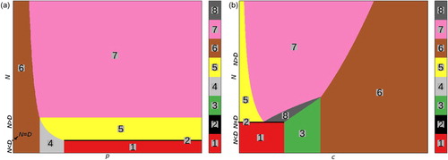
In both sub-figures, an increase of N correlates with a more efficient acquisition, as more items can be acquired by spending a constant acquisition effort. In the first sub-figure 1(a), remanufacturing is comparatively unattractive in an economical sense for very low values of p; thus, besides the selective acquisition, not all of the acquired goods are remanufactured (Scenario 6). With increasing sales price p for remanufactured goods and at the same time a low level of N, the optimal scenario switches to selective acquisition but full remanufacturing (Scenario 4). A further increase leads either to full acquisition/full remanufacturing (Scenario 1 when N<D/Scenario 2 when N=D) or selective acquisition/full remanufacturing when N>D (Scenario 5). Full acquisition/full remanufacturing (in Scenarios 1 and 2) is induced by low values for N: all available goods are acquired, and the entire acquired quantity is economically remanufactured due to sufficient sales price p. A rising number of available goods in the case of N>D increases the efficiency of the acquisition process: therefore, the acquisition can be selective, but all acquired goods are remanufactured (full remanufacturing in Scenarios 4 and 5). Finally, the high number of available products for acquisition makes selective acquisition and selective remanufacturing economically attractive (Scenario 7).

Similarly, the cost increase for remanufacturing in sub-figure 1(b) leads to a shift of optimal scenarios from full acquisition/full remanufacturing (Scenarios 1 or 2 which only occur when $N\le D$) to full acquisition/seletive remanufacturing (Scenario 3). Intuitively, with further rising remanufacturing cost the optimal scenario switches to selective acquisiton as well as remanufacturing (Scenario 6). In the case of N>D, the order of scenarios varies with increasing c. For low values of c, reprocessing is so cost-efficient that additional benefit can be gained solely from restricted acquisition but not from selective remanufacturing. Thus, selective acquisition/full remanufacturing (Scenario 5) is optimal. With increasing maximum cost for remanufacturing, the optimal scenario depends on the number of products available for acquisition: when N is comparatively low, all available products are acquired but selectively remanufactured, and full demand is satisfied (Scenario 8). A further increase of c can lead to still full acquisition/selective remanufacturing but accepting demand shortages when N is at a comparatively low level (Scenario 8 to Scenario 3). In the other case with a great number of available used products N, selection is applied to both acquisition and remanufacturing (Scenario 7), and no demand shortages occur. The impact of a further cost increase for reprocessing is obvious: the optimal scenario switches to selective acquisition/remanufacturing and incomplete demand satisfaction (Scenario 6).

4.3. Integration of stochastic newsvendor-like demand

Usually the demand for remanufactured products cannot be determined exactly but has to be estimated, what is also supported by the properties found in the case study concerning R.U.S.Z: First, reprocessing is a growing business sector, but a total demand for reprocessed items cannot be determined precisely but only estimated. In addition, there is a lack of knowledge on the projection of consumer demand, although research on the attitude of consumers related to reprocessed goods is in focus of a rising number of scientific works (see, e.g. Guide and Li 2010; Ovchinnikov 2011; Agrawal, Atasu, and Van Ittersum 2012; Subramanian and Subramanyam 2012). This will allow companies to more and more reduce uncertainty related to customer demand. Furthermore, R.U.S.Z has to provide the items in the way of a build-to-stock production. Thus, the sales with related acquisition/reprocessing costs have to be balanced and compared with the risk and cost of overproduction. Finally, R.U.S.Z faces almost constant prices for reprocessed items in the amount of 1/2 to 1/3 of the new product's price.

The integration of stochastic demand results in two different trade-offs included in the model, both interrelated with heterogeneous quality of used products: a demand trade-off and an acquisition-reprocessing trade-off. On the one hand, the former involves increasing/decreasing expected sales in an uncertain environment by raising/reducing the production quantity but, on the other hand, at the same time higher/lower acquisition and reprocessing costs for the supply with remanufactured goods in heterogeneous condition. The second trade-off concerns acquisition cost vs. cost for remanufacturing. An increased acquisition effort leads to more acquired used products but at the same time to higher acquisition costs. Nevertheless, the raised quantity of used products available for reprocessing allows to decrease cost for remanufacturing, as the remanufacturer can be more selective and remanufactures only products in the best condition.

In contrast to the model presented in Section 4, we consider uncertain, newsvendor-like demand with known probability density function (PDF) $g_D(\cdot )$ and cumulative distribution function (CDF) $G_D(\cdot )$. This uncertain demand combined with a specific offered reprocessing quantity q results in expected sales $S_D\left(q\right)$. The difference to the preceding model is that offering q items may deviate from the actual, uncertain sales quantity. Thus, not necessarily all of the offered products are sold. Still, we assume that reprocessed products are sold for a price p. Consequently, the expected revenue with an offered quantity q is expressed by (19) $p{S}_D\left(q\right).$(19) Equation (2(2) $-\gamma \left(e\right)eN.$(2) ) representing the total acquisition effort remains the same, and also the approach concerning the remanufacturing cost expressed by Equation (5(5) $-\frac{qc}{{\int }_0^{t}f\left(x\right)\mathrm{d}x}{\int }_0^{F^{-1}\left(q/\gamma \left(e\right)N\right)}xf\left(x\right)\mathrm{d}x.$(5) ) is equal to the one chosen in the preceding section. The combination of these three components result in objective function (20(20) $\underset{e,q}{max}\pi :p{S}_D\left(q\right)-\gamma \left(e\right)eN-\gamma \left(e\right)Nc{\int }_0^{t}xf\left(x\right)\mathrm{d}x$(20) ), and by additionally considering $t=F^{-1}\left(q/\gamma \left(e\right)N\right)$, a profit-maximising model with two decision variables e and q can be created. (20) $\underset{e,q}{max}\pi :p{S}_D\left(q\right)-\gamma \left(e\right)eN-\gamma \left(e\right)Nc{\int }_0^{t}xf\left(x\right)\mathrm{d}x$(20) s.t. (21) $\begin{array}{rl}q& \le \gamma \left(e\right)N\end{array}$(21) (22) $\begin{array}{rl}\gamma \left(e\right)& \le 1\end{array}$(22) (23) $\begin{array}{rl}e,q& \ge 0\end{array}$(23) The constraints are very similar to the ones in the preceding model: inequality (21(21) $\begin{array}{rl}q& \le \gamma \left(e\right)N\end{array}$(21) ) ensures that the reprocessing quantity is less or equal than the amount of acquired used products, while inequality (22(22) $\begin{array}{rl}\gamma \left(e\right)& \le 1\end{array}$(22) ) prevents that the total number of acquired goods exceeds the available products in the market.

Analogous to the section including the deterministic model, the analysis of the curvature of the objective function (provided in Appendix 2) does not yield any significant general statements. In order to obtain some analytic insights, the same explicit, uniformly distributed quality distribution of the acquired items as in the model with deterministic demand is integrated (see Equations (12(12) $\begin{array}{rl}\mathrm{P}\mathrm{D}\mathrm{F}:f\left(x\right)& =\left\{\begin{array}{ll}1& \text{if }0\le x\le 1\\ 0& \text{else.}\end{array}\right.\end{array}$(12) ), (13(13) $\begin{array}{rl}\mathrm{C}\mathrm{D}\mathrm{F}:F\left(x\right)& =\left\{\begin{array}{ll}0& \text{if }x<0\\ x& \text{if }0\le x\le 1\\ 1& \text{if }x>0\end{array}\right.\end{array}$(13) )). Using this, the expression including the remanufacturing cost simplifies to $-q^{2}c/2\gamma \left(e\right)N$, as $F^{-1}\left(q/\gamma \left(e\right)N\right)=q/\gamma \left(e\right)N$. As in the deterministic approach, the explicit acquisition function $\gamma \left(e\right)=e/m_{acq}$ is integrated in the model. Hence, these specifications result in the following model. (24) $\underset{e,q}{max}\pi :p{S}_D\left(q\right)-\frac{e^{2}N}{m_{acq}}-\frac{q^{2}c{m}_{acq}}{2eN}$(24) s.t. (25) $\begin{array}{rl}q& \le \frac{eN}{m_{acq}}\end{array}$(25) (26) $\begin{array}{rl}\frac{e}{m_{acq}}& \le 1\end{array}$(26) (27) $\begin{array}{rl}e,q& \ge 0\end{array}$(27) The objective function is concave and the constraints are convex, thus Karush–Kuhn–Tucker conditions are satisfied (see proofs in Appendix 2). Therefore, the according Lagrangian function L including the Karush–Kuhn–Tucker multipliers is composed as follows: (28) $L(e,q,{\lambda }_i):p{S}_D\left(q\right)-\frac{e^{2}N}{m_{acq}}-\frac{q^{2}c{m}_{acq}}{2eN}+{\lambda }_{1}e+{\lambda }_{2}q+{\lambda }_3\left(\frac{eN}{m_{acq}}-q\right)+{\lambda }_4\left(1-\frac{e}{m_{acq}}\right)$(28)

4.4. Analytical insights

First of all we find that ${\lambda }_1=0$ and ${\lambda }_2=0$, as any positive values of these shadow prices would suppress acquisition/reprocessing. Thus, the remaining analysis depends on the values for the shadow prices ${\lambda }_3$ (corresponding constraint (25(25) $\begin{array}{rl}q& \le \frac{eN}{m_{acq}}\end{array}$(25) )) and ${\lambda }_4$ (corresponding constraint (26(26) $\begin{array}{rl}\frac{e}{m_{acq}}& \le 1\end{array}$(26) )). All the proofs regarding the analytical insights are provided in Appendix A.3.

The optimal strategy consists of four different scenarios, as presented in Table 3. Full acquisition stands for the acquisition of the available amount N of used goods, while selective acquisition means partial acquisition of N. Similarly, in the case of full remanufacturing all acquired used products are reprocessed, while selective remanufacturing results in partial reprocessing of the returns. Furthermore, the conditions with respect to the shadow prices and the decision variables are given.

Table 3. Optimal strategy of the stochastic model defined by 4 scenarios.

Scenario	Acquisition	Remanufacturing	Conditions
1	Selective	Selective	$e<m_{acq}$, $q<{\displaystyle \frac{eN}{m_{acq}}}$
	$e={\displaystyle \frac{qc{m}_{acq}}{Np(1-G_D(q\left)\right)}}$	$q=\sqrt{{\displaystyle \frac{4e^3{N}^2}{c{m}_{acq}^2}}}$	${\lambda }_3=0$, ${\lambda }_4=0$
2	Selective	Full	$e\le m_{acq}$, $q={\displaystyle \frac{eN}{m_{acq}}}$
	$e={\displaystyle \frac{q{m}_{acq}}{N}}$	$G_D\left(q\right)+{\displaystyle \frac{2q{m}_{acq}}{Np}}=1-{\displaystyle \frac{c}{2p}}$	${\lambda }_3>0$, ${\lambda }_4=0$
3	Full	Selective	$q<{\displaystyle \frac{eN}{m_{acq}}}$
	$e=m_{acq}$	$G_D\left(q\right)+{\displaystyle \frac{qc}{pN}}=1$	${\lambda }_3=0$, ${\lambda }_4>0$
4	Full	Full	${\lambda }_3=p(1-G_D(N\left)\right)-c$
	$e=m_{acq}$	q=N	${\lambda }_4={\displaystyle \frac{Nc}{2}}-2m_{acq}N+{\lambda }_{3}N$

As the optimal, profit-maximising strategy is not represented by a closed-form solution, the values for $0\le e\le m_{acq}$ and $0\le q\le N$ or $0\le {\lambda }_3\le p-c$ and $0\le {\lambda }_4\le N(p-2m_{acq})$ are obtained by applying an appropriate search method: first of all, calculate the acquisition effort and the offered quantity for Scenario 1 by solving the non-linear system of equations (apparently, under the conditions e>0 and q>0). In case that both conditions $e<m_{acq}$ and $q<eN/m_{acq}$ are satisfied, this is the optimal result. Otherwise, proceed with the calculation of the values of Scenario 2 as well as Scenario 3; again, check for the related conditions and choose the scenario which satisfies them. If both satisfy the related conditions, the scenario with the higher profit is the optimal one. Otherwise, in case that neither Scenario 2 nor Scenario 3 provide feasible solutions, Scenario 4 is optimal.

5. Numerical examples of the model with stochastic newsvendor-like demand

To illustrate the analytical results of the model and to emphasise the applicability of the model, we present a numerical study. For operational and data confidentiality reasons we cannot emphasise detailed model results on the basis of specific reprocessing cost and prices observed at R.U.S.Z. Nevertheless, a structured numerical analysis allows to gain a deeper understanding of the model: the variation of selected key variables across a broad spectrum of values demonstrates fundamental effects occurring in the model. The investigation of such relative effects does not require absolute values.

The numerical analysis provides insights into the sensitivity regarding different parameters: in detail, we take a closer look at c to obtain results for different maximal remanufacturing costs. Furthermore, various values for the maximum available used items are considered to gather information regarding both the supply and the demand side. We refrain from a sensitivity analysis with respect to the sales price of reprocessed products, as this does not provide any further information. This is caused by the fact that the variations of the maximum reprocessing cost cover the important factor of varying relations between price and reprocessing cost. The same is true for the relation of demand and the maximum number of available used goods, which is covered by the sensitivity analysis with different values of N. As specified in Section 4.1, the acquisition effort function is defined as $\gamma \left(e\right)=e/m_{acq}$. The quality follows the uniform distribution function specified in Equation (12(12) $\begin{array}{rl}\mathrm{P}\mathrm{D}\mathrm{F}:f\left(x\right)& =\left\{\begin{array}{ll}1& \text{if }0\le x\le 1\\ 0& \text{else.}\end{array}\right.\end{array}$(12) ). Finally, an explicit demand distribution is included in order to conduct a numerical analysis. To keep the model as simple and comprehensible as possible, we assume uniformly distributed demand $D\sim U(a,b)$.

In Table 4, the setup of the numerical analysis is shown.

Table 4. Setup of parameters for numerical analysis.

Parameter	Value	Base case value
Sales price of remanufactured item	p=10	p=10
Max. remanufacturing cost	$c=1.00,1.05,\dots ,19.95,20.00$	c=5
Max. available used items	$N=5.00,5.05,\dots ,99.95,100.00$	N=30
Lower limit of uniformly distributed demand	a=0,5	a=0
Upper limit of uniformly distributed demand	b=a+20	b=20
Slope parameter of acquisition function	$m_{acq}=1,2,\dots ,9,10$	$m_{acq}=5$

Concerning the results, we focus on the sensitivity analysis of the base case with respect to maximum number of available items for acquisition (N) and maximum reprocessing cost (c). The first numerical analysis is shown in Table 5, where the impact of rising maximum available used items is explored. Due to the fact that all occurring effects can be found in the range of $5\le N\le 50$, we restrict the analysis to this range and present a representative sample. The acquired amount of used products rises due to the increase of N, although the marginal acquisition effort and the acquisition rate decline. First, the total acquisition cost rises with a peak at N=20. Due to rising possible supply with used items, acquisition cost can be reduced and therefore, decreases slightly beyond this value. All of these acquired products are remanufactured when $N\le 40$. In the case N exceeds this amount, it is optimal to benefit from a better quality of the goods to remanufacture; this is based upon the selection which of the acquired products to reprocess. Consequently, this results in lower total remanufacturing cost caused by changing the strategy from Scenario 2 including full remanufacturing to Scenario 1 with limited remanufacturing. Therefore, total remanufacturing cost increases up to N=40, while beyond this value the total remanufacturing cost declines. Obviously, a rising number of used products for potential acquisition is always profitable due to acquisition and/or remanufacturing cost savings.

Table 5. Key figures concerning the sensitivity of the stochastic base case over N.

N	Scenario	Acq. effort	Acq. qty.	Offered qty.	Acq. rate	Reman. rate	Revenue	Total acq. cost	Total reman. cost	Profit
5	2	3.00000	3.000	3.000	60.000%	100.000%	27.750	9.000	7.500	11.250
10	2	2.50000	5.000	5.000	50.000%	100.000%	43.750	12.500	12.500	18.750
15	2	2.14285	6.429	6.429	42.860%	100.000%	53.954	13.775	16.071	24.107
20	2	1.87500	7.500	7.500	37.500%	100.000%	60.938	14.063	18.750	28.125
25	2	1.66667	8.333	8.333	33.332%	100.000%	65.972	13.889	20.833	31.250
30	2	1.50000	9.000	9.000	30.000%	100.000%	69.750	13.500	22.500	33.750
35	2	1.36364	9.545	9.545	27.271%	100.000%	72.676	13.017	23.864	35.795
40	2	1.25000	10.000	10.000	25.000%	100.000%	75.000	12.500	25.000	37.500
45	1	1.17801	10.602	10.292	23.560%	97.076%	76.440	12.489	24.979	38.972
50	1	1.11634	11.163	10.550	22.326%	94.509%	77.673	12.462	24.924	40.286

A further analysis presented in Table 6 and Figure 2 concerns the maximal remanufacturing cost c, while the amount of available used items is fixed. Again, we select a representative sample which includes all relevant effects. The per-item acquisition effort, the acquisition amount, and the offered quantity decline with rising maximum cost for remanufacturing, as it is more beneficial to acquire and offer less items due to the increased cost. Scenario 2 of the strategy (limited acquisition of used products, remanufacturing of all acquired items) is optimal in the cases of $c=2$ and c=4, while for the remaining numerical setups with raised c Scenario 1 – limited acquisition and limited remanufacturing – maximises the profit. Similar to the example presented above, the limited remanufacturing is triggered by the improvement of the average quality of the remanufactured items to counteract the risen maximum remanufacturing cost.

Figure 2. Revenue, profit, and total costs with varying c.

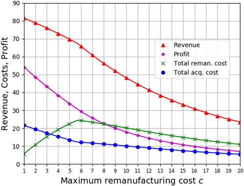
Table 6. Key figures concerning the sensitivity of the stochastic base case over c.

c	Scenario	Acq. effort	Acq. qty.	Offered qty.	Acq. rate	Reman. rate
2	2	1.80000	10.800	10.800	36.000%	100.000%
4	2	1.60000	9.600	9.600	32.000%	100.000%
6	1	1.42270	8.536	8.313	28.453%	97.388%
8	1	1.36628	8.198	6.776	27.327%	82.654%
10	1	1.29611	7.777	5.599	25.923%	71.994%
12	1	1.22225	7.334	4.681	24.447%	63.826%
14	1	1.14958	6.898	3.953	22.993%	57.306%
16	1	1.08042	6.483	3.369	21.610%	51.967%
18	1	1.01581	6.095	2.896	20.317%	47.514%
20	1	0.95610	5.737	2.509	19.123%	43.734%

The related revenue, acquisition and remanufacturing costs, and profit are shown in Figure 2. Interestingly, the total remanufacturing cost first increases and then – from c=5.75 onward – declines with rising c. The change from Scenario 2 to Scenario 1 induces this effect, as an improved quality of the products to remanufacture is beneficial with increased maximum cost for remanufacturing. However, as total spending for acquisition solely decreases, less used products are available for remanufacturing. Thus, both revenue and profit decrease.

Scenarios 3 and 4 of the strategy also appear in the numerical analysis, e.g. in the setup a=5, b=25, c=7, $m_{acq}=1$, and N=10, 15, 20 presented in Table 7. All of the available items are acquired, remanufactured, and offered in the case N=10 (Scenario 4). While N=15 results in the acquisition of all used products but limited reprocessing, Scenario 1 including limited acquisition and remanufacturing of a part of the acquired items is optimal when N=20.

Table 7. Occurrence of further scenarios of the optimal strategy.

N	Scenario	Acq. effort	Acq. qty.	Offered qty.	Acq. rate	Reman. rate
10	4	1.00000	10.000	10.000	100.000%	100.000%
15	3	1.00000	15.000	12.931	100.000%	86.207%
20	1	0.97482	19.496	14.551	97.482%	74.635%

6. Conclusion

The presented research contributes to decision-making in Reverse Logistics and Closed-loop Supply Chains by modelling the perspective of an independent reprocessing company. As the literature review shows, the number of works of the scientific community focusing on integrated decision support systems in RL/CLSC-context is rather limited and thus provides research opportunities in this field. In the models aspects of active acquisition of used products, quality grading of used acquired items and reprocessing decisions are jointly considered, what allows studying an integrated decision-making with respect to these processes. The introduction of both deterministic and stochastic demand adds additional variety. The models turned out to be analytically intractable for general and undefined cases but tractable when specifying the terms for acquisition effort and the heterogeneous quality of acquired used products. Hence, the optimal strategies of the models provide analytic insights into the interdependencies between acquisition, grading and disposition processes and resultant effects.

Despite the level of integration, the models are elementary approaches in comparison with real-world decisions. Nevertheless, the work reveals the importance of integrated decision-making. The effects occurring caused by the interrelated processes are complex and non-trivial, and the resulting cross-impacts impede an intuitive decision-making. Complementary, the sensitivity analyses conducted in the numerical studies emphasise this by giving an impression of the broad range of effects on model decisions and numerical results under different conditions.

In the light of the upcoming global environmental and social challenges, future work should deal with some topics extending the integration of decision-making. Obvious extensions of the conducted research are, e.g. the consideration of multiple periods in order to make product life cycle-based studies possible, or the introduction of additional disposition options like direct reuse or refurbishment. Naturally, any organisations in RL/CLSC are interacting with other organisations, what shows the need for research on the impact of network structure on integrated decision-making. Beyond that, in existing scientific work a structured analysis answering the question of the additional value of further decision integration is not available. Without much doubt, an integration of such further aspects related to RL/CLSC calls for a great variety of methods and approaches to cope with modelling complex decision-making. Finally, closing the loop requires the incorporation of environmental and social aspects, what is the case for example in the R.U.S.Z-case. Thus, a holistic examination of effective performance indicators in order to measure the impact of integrated decision-making would definitely support the transformation to a sustainable Circular Economy respecting people, planet and profit.

Disclosure statement

No potential conflict of interest was reported by the authors.

Additional information

Funding

This work has been supported by funds of the Oesterreichische National Bank (Anniversary Fund, project number: 14974). The authors gratefully acknowledge this financial support. The authors also acknowledge the financial support by the University of Graz.

Notes

1 https://www.rematec.com/blogs/blog/why-oems-go-for-remanufacturing/, https://www.therecycler.com/posts/oems-adopt-circular-economy-methods/, https://www.ellenmacarthurfoundation.org/about/partners

Appendices

A. Appendix 1. Proofs of Section 4

First derivatives of Equation (11(11) $\begin{array}{rl}& L:pq-\gamma \left(e\right)eN-\gamma \left(e\right)Nc{\int }_0^{F^{-1}\left(q/\gamma \left(e\right)N\right)}xf\left(x\right)\mathrm{d}x\\ & +{\lambda }_1(1-\gamma (e\left)\right)+{\lambda }_2(D-q)+{\lambda }_3\left(\gamma \right(e)N-q).\end{array}$(11) ) with respect to q and e are (A1) $\frac{\mathrm{\partial }L}{\mathrm{\partial }q}:p-c{F}^{-1}\left(\frac{q}{\gamma \left(e\right)N}\right)-{\lambda }_2-{\lambda }_3$(A1) and (A2) $\begin{array}{rl}& \frac{\mathrm{\partial }L}{\mathrm{\partial }e}:-\left(\frac{\mathrm{d}}{\mathrm{d}e}\gamma \left(e\right)\right)eN-\gamma \left(e\right)N-\left(\frac{\mathrm{d}}{\mathrm{d}e}\gamma \left(e\right)\right)Nc{\int }_0^{F^{-1}\left(q/\gamma \left(e\right)N\right)}xf\left(x\right)\mathrm{d}x-\gamma \left(e\right)c{F}^{-1}\left(\frac{q}{\gamma \left(e\right)N}\right)\left(\frac{\mathrm{d}}{\mathrm{d}e}\frac{q}{\gamma \left(e\right)}\right)+({\lambda }_{3}N-{\lambda }_1)\left(\frac{\mathrm{d}}{\mathrm{d}e}\gamma \left(e\right)\right).\end{array}$(A2) To analyse the concavity of the objective function, the corresponding Hessian matrix is derived. (A3) $\begin{array}{rl}& \frac{{\mathrm{\partial }}^2\pi }{\mathrm{\partial }{q}^2}:-c\frac{1}{f\left(F^{-1}\left(\frac{q}{\gamma \left(e\right)N}\right)\right)\gamma \left(e\right)N}\end{array}$(A3) (A4) $\begin{array}{rl}& \frac{{\mathrm{\partial }}^2\pi }{\mathrm{\partial }q\mathrm{\partial }e}:-c\frac{1}{f\left(F^{-1}\left(\frac{q}{\gamma \left(e\right)N}\right)\right)}\left(\frac{\mathrm{d}}{\mathrm{d}e}\frac{q}{\gamma \left(e\right)N}\right)\end{array}$(A4) (A5) $\begin{array}{rl}& \frac{{\mathrm{\partial }}^2\pi }{\mathrm{\partial }e\mathrm{\partial }q}:-\left(\frac{\mathrm{d}}{\mathrm{d}e}\gamma \left(e\right)\right)c{F}^{-1}\left(\frac{q}{\gamma \left(e\right)N}\right)\left(\frac{1}{\gamma \left(e\right)}\right)-c\frac{1}{f\left(F^{-1}\left(\frac{q}{\gamma \left(e\right)N}\right)\right)N}\left(\frac{\mathrm{d}}{\mathrm{d}e}\frac{q}{\gamma \left(e\right)}\right)-\gamma \left(e\right)c{F}^{-1}\left(\frac{q}{\gamma \left(e\right)N}\right)\left(\frac{\mathrm{d}}{\mathrm{d}e}\frac{1}{\gamma \left(e\right)}\right)\end{array}$(A5) Applying the reciprocal rule (A6) $\frac{\mathrm{d}}{\mathrm{d}e}\frac{1}{\gamma \left(e\right)}=-\left(\frac{\mathrm{d}}{\mathrm{d}e}\gamma \left(e\right)\right)\frac{1}{\left(\gamma \right(e){)}^2}$(A6) results in (A7) $\begin{array}{rl}& \frac{{\mathrm{\partial }}^2\pi }{\mathrm{\partial }e\mathrm{\partial }q}:-c\frac{1}{f\left(F^{-1}\left(\frac{q}{\gamma \left(e\right)N}\right)\right)}\left(\frac{\mathrm{d}}{\mathrm{d}e}\frac{q}{\gamma \left(e\right)N}\right).\end{array}$(A7) (A8) $\begin{array}{rl}& \frac{{\mathrm{\partial }}^2\pi }{\mathrm{\partial }{e}^2}:-eN\left(\frac{{\mathrm{d}}^2}{\mathrm{d}{e}^2}\gamma \left(e\right)\right)-2N\left(\frac{\mathrm{d}}{\mathrm{d}e}\gamma \left(e\right)\right)-cN\left(\frac{{\mathrm{d}}^2}{\mathrm{d}{e}^2}\gamma \left(e\right)\right){\int }_0^{F^{-1}\left(q/\gamma \left(e\right)N\right)}xf\left(x\right)\mathrm{d}x\\ & -2c{F}^{-1}\left(\frac{q}{\gamma \left(e\right)N}\right)\left(\frac{\mathrm{d}}{\mathrm{d}e}\gamma \left(e\right)\right)\left(\frac{\mathrm{d}}{\mathrm{d}e}\frac{q}{\gamma \left(e\right)}\right)\\ & -c\gamma \left(e\right){\left(\frac{\mathrm{d}}{\mathrm{d}e}\frac{q}{\gamma \left(e\right)}\right)}^2\frac{1}{f\left(F^{-1}\left(\frac{q}{\gamma \left(e\right)N}\right)\right)}\\ & -c\gamma \left(e\right)F^{-1}\left(\frac{q}{\gamma \left(e\right)N}\right)\left(\frac{{\mathrm{d}}^2}{\mathrm{d}{e}^2}\frac{q}{\gamma \left(e\right)}\right)\end{array}$(A8) The objective function is concave if following conditions are satisfied: ${\mathrm{\partial }}^2\pi /\mathrm{\partial }{q}^2\le 0$ and $\left({\mathrm{\partial }}^2\pi /\mathrm{\partial }{q}^2\right)\left({\mathrm{\partial }}^2\pi /\mathrm{\partial }{e}^2\right)-{{\mathrm{\partial }}^2\pi /\mathrm{\partial }{q}^2}^2\ge 0$. Due to the complexity of the computations above, general criteria for the curvature of the objective function cannot be provided.

A.1. Check on curvature of objective function presented in Section 4.1

The corresponding Hessian Matrix of Equation (14(14) $\underset{e,q}{max}\pi :pq-\frac{e^{2}N}{m_{acq}}-\frac{q^{2}c{m}_{acq}}{2Ne}$(14) ) with respect to the two decision variables e and q allows to check the concavity of the objective function. (A9) $\begin{array}{rl}& \frac{\mathrm{\partial }\pi }{\mathrm{\partial }q}:p-\frac{qc{m}_{acq}}{Ne}\end{array}$(A9) (A10) $\begin{array}{rl}& \frac{\mathrm{\partial }\pi }{\mathrm{\partial }e}:-\frac{2Ne}{m_{acq}}+\frac{q^{2}c{m}_{acq}}{2N{e}^2}\end{array}$(A10) (A11) $\begin{array}{rl}& \frac{{\mathrm{\partial }}^2\pi }{\mathrm{\partial }{q}^2}:-\frac{c{m}_{acq}}{Ne}=A<0(\mathrm{\forall }e>0)\end{array}$(A11) (A12) $\begin{array}{rl}& \frac{{\mathrm{\partial }}^2\pi }{\mathrm{\partial }q\mathrm{\partial }e}:\frac{qc{m}_{acq}}{N{e}^2}=B\end{array}$(A12) (A13) $\begin{array}{rl}& \frac{{\mathrm{\partial }}^2\pi }{\mathrm{\partial }e\mathrm{\partial }q}:\frac{qc{m}_{acq}}{N{e}^2}=B\end{array}$(A13) (A14) $\begin{array}{rl}& \frac{{\mathrm{\partial }}^2\pi }{\mathrm{\partial }{e}^2}:-\frac{2N}{m_{acq}}-\frac{q^{2}c{m}_{acq}}{N{e}^3}=C\end{array}$(A14) (A15) $\begin{array}{rl}& \left(-\frac{c{m}_{acq}}{Ne}\right)\left(-\frac{2N}{m_{acq}}-\frac{q^{2}c{m}_{acq}}{N{e}^3}\right)-{\left(\frac{qc{m}_{acq}}{N{e}^2}\right)}^2=\frac{2c}{e}>0(\mathrm{\forall }e>0)\end{array}$(A15) Following Equations (A11(A11) $\begin{array}{rl}& \frac{{\mathrm{\partial }}^2\pi }{\mathrm{\partial }{q}^2}:-\frac{c{m}_{acq}}{Ne}=A<0(\mathrm{\forall }e>0)\end{array}$(A11) ) and (A15(A15) $\begin{array}{rl}& \left(-\frac{c{m}_{acq}}{Ne}\right)\left(-\frac{2N}{m_{acq}}-\frac{q^{2}c{m}_{acq}}{N{e}^3}\right)-{\left(\frac{qc{m}_{acq}}{N{e}^2}\right)}^2=\frac{2c}{e}>0(\mathrm{\forall }e>0)\end{array}$(A15) ), the leading principal minors are $-c{m}_{acq}/Ne=A<0(\mathrm{\forall }e>0)$ and $2c/e>0$. Thus, the Hessian matrix is negative definite, so the objective function is concave for all e>0.

A.2. Proof of strategy presented in Section 4.2

The derivatives of the Lagrange-function (A16) $L:pq-\frac{e^{2}N}{m_{acq}}-\frac{q^{2}c{m}_{acq}}{2Ne}+{\lambda }_1\left(1-\frac{e}{m_{acq}}\right)+{\lambda }_2(D-q)+{\lambda }_3\left(\frac{eN}{m_{acq}}-q\right)$(A16) with respect to q (A17) $\frac{\mathrm{\partial }L}{\mathrm{\partial }q}:p-\frac{qc{m}_{acq}}{Ne}-{\lambda }_2-{\lambda }_3=0$(A17) and e (A18) $\frac{\mathrm{\partial }L}{\mathrm{\partial }e}:-\frac{2Ne}{m_{acq}}+\frac{q^{2}c{m}_{acq}}{2N{e}^2}-\frac{1}{m_{acq}}{\lambda }_1+\frac{N}{m_{acq}}{\lambda }_3=0$(A18) lead to the optimal constrained profit-maximising strategy.

• Scenario 1:

  • ${\lambda }_1>0$, ${\lambda }_2=0$, ${\lambda }_3>0$: q=N, $e=m_{acq}$

  • Equation (A17(A17) $\frac{\mathrm{\partial }L}{\mathrm{\partial }q}:p-\frac{qc{m}_{acq}}{Ne}-{\lambda }_2-{\lambda }_3=0$(A17) ) gives: ${\lambda }_3=p-qc{m}_{acq}/Ne=p-c\Rightarrow p>c$

  • Equation (A18(A18) $\frac{\mathrm{\partial }L}{\mathrm{\partial }e}:-\frac{2Ne}{m_{acq}}+\frac{q^{2}c{m}_{acq}}{2N{e}^2}-\frac{1}{m_{acq}}{\lambda }_1+\frac{N}{m_{acq}}{\lambda }_3=0$(A18) ) gives: ${\lambda }_1-N{\lambda }_3=q^{2}c{m}_{acq}^2/2N{e}^2-2Ne=N(c/2-2m_{acq})\Rightarrow p-c/2>2m_{acq}$

  • q=N, $e=m_{acq}$

• Scenario 2:

  • ${\lambda }_1>0$, ${\lambda }_2>0$, ${\lambda }_3\ge 0$: q=D=N, $e=m_{acq}$

  • Equation (A17(A17) $\frac{\mathrm{\partial }L}{\mathrm{\partial }q}:p-\frac{qc{m}_{acq}}{Ne}-{\lambda }_2-{\lambda }_3=0$(A17) ) gives: ${\lambda }_2+{\lambda }_3=p-qc{m}_{acq}/Ne=p-c\Rightarrow p>c$

  • Equation (A18(A18) $\frac{\mathrm{\partial }L}{\mathrm{\partial }e}:-\frac{2Ne}{m_{acq}}+\frac{q^{2}c{m}_{acq}}{2N{e}^2}-\frac{1}{m_{acq}}{\lambda }_1+\frac{N}{m_{acq}}{\lambda }_3=0$(A18) ) gives: ${\lambda }_1-N{\lambda }_3=q^{2}c{m}_{acq}^2/2N{e}^2-2Ne=N(c/2-2m_{acq})$

  • q=D=N, $e=m_{acq}$

• Scenario 3:

  • ${\lambda }_1>0$, ${\lambda }_2=0$, ${\lambda }_3=0$: $e=m_{acq}$

  • Equation (A17(A17) $\frac{\mathrm{\partial }L}{\mathrm{\partial }q}:p-\frac{qc{m}_{acq}}{Ne}-{\lambda }_2-{\lambda }_3=0$(A17) ) gives: $e=qc{m}_{acq}/pN\Rightarrow qc/pN=1;q/N<1\Rightarrow p<c$

  • Equation (A18(A18) $\frac{\mathrm{\partial }L}{\mathrm{\partial }e}:-\frac{2Ne}{m_{acq}}+\frac{q^{2}c{m}_{acq}}{2N{e}^2}-\frac{1}{m_{acq}}{\lambda }_1+\frac{N}{m_{acq}}{\lambda }_3=0$(A18) ) gives: ${\lambda }_1=q^{2}c{m}_{acq}^2/2N^2{e}^2-2Ne=q^{2}c/2N^2-2N{m}_{acq}\Rightarrow p>2\sqrt{N{m}_{acq}c}$

  • ${\lambda }_1>0$, ${\lambda }_2=0$, ${\lambda }_3=0$

  • $q=pN/c$, $e=m_{acq}$

• Scenario 4:

  • ${\lambda }_1=0$, ${\lambda }_2=0$, ${\lambda }_3>0$: $eN/m_{acq}=q$

  • Equation (A17(A17) $\frac{\mathrm{\partial }L}{\mathrm{\partial }q}:p-\frac{qc{m}_{acq}}{Ne}-{\lambda }_2-{\lambda }_3=0$(A17) ) gives: ${\lambda }_3=p-qc{m}_{acq}/Ne=p-c\Rightarrow p>c$

  • Equation (A18(A18) $\frac{\mathrm{\partial }L}{\mathrm{\partial }e}:-\frac{2Ne}{m_{acq}}+\frac{q^{2}c{m}_{acq}}{2N{e}^2}-\frac{1}{m_{acq}}{\lambda }_1+\frac{N}{m_{acq}}{\lambda }_3=0$(A18) ) gives: ${\lambda }_3=2e-q^{2}c{m}_{acq}^2/2N^2{e}^2\Rightarrow p>c/2$

  • As D>q: $\Rightarrow 2p-c<4D{m}_{acq}/N$

  • $q=N(2p-c)/4m_{acq}$, $e=\left(2p-c\right)/4$

• Scenario 5:

  • ${\lambda }_1=0$, ${\lambda }_2>0$, ${\lambda }_3>0$: q=D, $e=D{m}_{acq}/N$

  • Equation (A17(A17) $\frac{\mathrm{\partial }L}{\mathrm{\partial }q}:p-\frac{qc{m}_{acq}}{Ne}-{\lambda }_2-{\lambda }_3=0$(A17) ) gives: ${\lambda }_2+{\lambda }_3=p-qc{m}_{acq}/Ne=p-c\Rightarrow p>c$

  • Equation (A18(A18) $\frac{\mathrm{\partial }L}{\mathrm{\partial }e}:-\frac{2Ne}{m_{acq}}+\frac{q^{2}c{m}_{acq}}{2N{e}^2}-\frac{1}{m_{acq}}{\lambda }_1+\frac{N}{m_{acq}}{\lambda }_3=0$(A18) ) gives: ${\lambda }_3=2e-q^{2}c{m}_{acq}^2/2N^2{e}^2=\left(4D{m}_{acq}-cN\right)/2N$

  • Replacing ${\lambda }_3=p-c-{\lambda }_2$ in the term above yields $p-c/2-2D{m}_{acq}/N>0$

  • q=D, $e=D{m}_{acq}/N$

• Scenario 6:

  • ${\lambda }_1=0$, ${\lambda }_2=0$, ${\lambda }_3=0$

  • Equation (A17(A17) $\frac{\mathrm{\partial }L}{\mathrm{\partial }q}:p-\frac{qc{m}_{acq}}{Ne}-{\lambda }_2-{\lambda }_3=0$(A17) ) gives: $e=qc{m}_{acq}/pN\Rightarrow q/e=\left(pN/c{m}_{acq}\right)$

  • Equation (A18(A18) $\frac{\mathrm{\partial }L}{\mathrm{\partial }e}:-\frac{2Ne}{m_{acq}}+\frac{q^{2}c{m}_{acq}}{2N{e}^2}-\frac{1}{m_{acq}}{\lambda }_1+\frac{N}{m_{acq}}{\lambda }_3=0$(A18) ) gives: $e^3=q^{2}c{m}_{acq}^2/4N^2\Rightarrow e=p^2/\left(4c\right)\Rightarrow q=p^{3}N/4c^2{m}_{acq}$

  • Combining $e<m_{acq}$ with results above gives: $p^2/c<4m_{acq}$ and $p^3/c^2<4D{m}_{acq}/N$

  • $q=p^{3}N/4c^2{m}_{acq}$, $e=p^2/4c$

• Scenario 7:

  • ${\lambda }_1=0$, ${\lambda }_2>0$, ${\lambda }_3=0$: q=D, $\Rightarrow e>Dm/N$

  • Equation (A17(A17) $\frac{\mathrm{\partial }L}{\mathrm{\partial }q}:p-\frac{qc{m}_{acq}}{Ne}-{\lambda }_2-{\lambda }_3=0$(A17) ) gives: ${\lambda }_2=p-qc{m}_{acq}/Ne=p-Dc{m}_{acq}/Ne\Rightarrow p>Dc{m}_{acq}/Ne$

  • Equation (A18(A18) $\frac{\mathrm{\partial }L}{\mathrm{\partial }e}:-\frac{2Ne}{m_{acq}}+\frac{q^{2}c{m}_{acq}}{2N{e}^2}-\frac{1}{m_{acq}}{\lambda }_1+\frac{N}{m_{acq}}{\lambda }_3=0$(A18) ) gives: $e^3=q^{2}c{m}_{acq}^2/4N^2$

  • Combining $p-{\lambda }_2=Dc{m}_{acq}/Ne$ and $2Ne/m_{acq}=D^{2}c{m}_{acq}/2e^{2}N$ yields $pD{m}_{acq}>4N{e}^2$

  • q=D, $e=\sqrt[3]{D^{2}c{m}_{acq}^2/4N^2}$

• Scenario 8:

  • ${\lambda }_1>0$, ${\lambda }_2>0$, ${\lambda }_3=0$: q=D, $e=m_{acq}$, N>D

  • Equation (A17(A17) $\frac{\mathrm{\partial }L}{\mathrm{\partial }q}:p-\frac{qc{m}_{acq}}{Ne}-{\lambda }_2-{\lambda }_3=0$(A17) ) gives: ${\lambda }_2=p-qc{m}_{acq}/Ne=p-Dc/N>0$

  • Equation (A18(A18) $\frac{\mathrm{\partial }L}{\mathrm{\partial }e}:-\frac{2Ne}{m_{acq}}+\frac{q^{2}c{m}_{acq}}{2N{e}^2}-\frac{1}{m_{acq}}{\lambda }_1+\frac{N}{m_{acq}}{\lambda }_3=0$(A18) ) gives: ${\lambda }_1=q^{2}c{m}_{acq}^2/2N{e}^2-2Ne=\left(D^{2}c-4N^2{m}_{acq}\right)/2N>0\Rightarrow D^{2}c>4N^2{m}_{acq}$

  • q=D<N, $e=m_{acq}$

Appendix 2. Proofs of Section 4.3

The curvature of the general objective function is analysed using the related Hessian matrix. The first derivatives are (A19) $\begin{array}{rl}& \frac{\mathrm{\partial }\pi }{\mathrm{\partial }e}:(-N)\left[\left(\frac{\mathrm{d}}{\mathrm{d}e}\gamma \left(e\right)\right)\left(e+c{\int }_0^{F^{-1}\left(q/\gamma \left(e\right)N\right)}xf\left(x\right)\mathrm{d}x\right)-\gamma \left(e\right)N\left(1+c{F}^{-1}\left(\frac{q}{\gamma \left(e\right)N}\right)\left(\frac{\mathrm{d}}{\mathrm{d}e}\frac{q}{\gamma \left(e\right)N}\right)\right)\phantom{{\int }_0^{F^{-1}\left(q/\gamma \left(e\right)N\right)}}\right]\end{array}$(A19) and (A20) $\frac{\mathrm{\partial }\pi }{\mathrm{\partial }q}:p(1-G_D(q\left)\right)-c{F}^{-1}\left(\frac{q}{\gamma \left(e\right)N}\right).$(A20) The further derivation results in the following equations. (A21) $\begin{array}{rl}& \frac{\mathrm{\partial }\mathrm{\partial }\pi }{\mathrm{\partial }{e}^2}:-N\left[\left(\frac{{\mathrm{d}}^2}{\mathrm{d}{e}^2}\gamma \left(e\right)\right)e+2\left(\frac{\mathrm{d}}{\mathrm{d}e}\gamma \left(e\right)\right)\phantom{\frac{c\gamma \left(e\right)\left(\frac{\mathrm{d}}{\mathrm{d}e}\frac{q}{\gamma \left(e\right)N}\right)}{\frac{\mathrm{d}}{\mathrm{d}e}F\left(F^{-1}\left(\frac{q}{\gamma \left(e\right)N}\right)\right)}}+\left(\frac{{\mathrm{d}}^2}{\mathrm{d}{e}^2}\gamma \left(e\right)\right)c{\int }_0^{F^{-1}\left(q/\gamma \left(e\right)N\right)}xf\left(x\right)\mathrm{d}x+2c\left(\frac{\mathrm{d}}{\mathrm{d}e}\gamma \left(e\right)\right)F^{-1}\left(\frac{q}{\gamma \left(e\right)N}\right)\left(\frac{\mathrm{d}}{\mathrm{d}e}\frac{q}{\gamma \left(e\right)N}\right)\right.\\ & \left.+c\left(\frac{{\mathrm{d}}^2}{\mathrm{d}{e}^2}\frac{q}{\gamma \left(e\right)N}\right)\gamma \left(e\right)F^{-1}\left(\frac{q}{\gamma \left(e\right)N}\right)+\frac{c\gamma \left(e\right)\left(\frac{\mathrm{d}}{\mathrm{d}e}\frac{q}{\gamma \left(e\right)N}\right)}{\frac{\mathrm{d}}{\mathrm{d}e}F\left(F^{-1}\left(\frac{q}{\gamma \left(e\right)N}\right)\right)}\right]\end{array}$(A21) (A22) $\begin{array}{rl}& \frac{\mathrm{\partial }\mathrm{\partial }\pi }{\mathrm{\partial }e\mathrm{\partial }q}:-N\left[\left(\frac{\mathrm{d}}{\mathrm{d}e}\gamma \left(e\right)\right)c{F}^{-1}\left(\frac{q}{\gamma \left(e\right)N}\right)\left(\frac{1}{\gamma \left(e\right)N}\right)\phantom{\frac{c\gamma \left(e\right)\left(\frac{\mathrm{d}}{\mathrm{d}e}\frac{q}{\gamma \left(e\right)N}\right)}{\frac{\mathrm{d}}{\mathrm{d}e}F\left(F^{-1}\left(\frac{q}{\gamma \left(e\right)N}\right)\right)}}+\gamma \left(e\right)c{F}^{-1}\left(\frac{q}{\gamma \left(e\right)N}\right)\left(\frac{\mathrm{d}}{\mathrm{d}e}\frac{1}{\gamma \left(e\right)N}\right)+\gamma \left(e\right)c\frac{1}{\frac{\mathrm{d}}{\mathrm{d}q}F\left(F^{-1}\left(\frac{q}{\gamma \left(e\right)N}\right)\right)}\left(\frac{\mathrm{d}}{\mathrm{d}e}\frac{q}{\gamma \left(e\right)N}\right)\right]\end{array}$(A22) Applying the reciprocal rule (A23) $\frac{\mathrm{d}}{\mathrm{d}e}\frac{1}{\gamma \left(e\right)}=-\left(\frac{\mathrm{d}}{\mathrm{d}e}\gamma \left(e\right)\right)\frac{1}{\left(\gamma \right(e){)}^2}$(A23) simplifies the expression above to (A24) $\begin{array}{rl}& \frac{\mathrm{\partial }\mathrm{\partial }\pi }{\mathrm{\partial }e\mathrm{\partial }q}:-c\frac{\left(\frac{\mathrm{d}}{\mathrm{d}e}\frac{q}{\gamma \left(e\right)N}\right)}{f\left(F^{-1}\left(\frac{q}{\gamma \left(e\right)N}\right)\right)}.\end{array}$(A24) (A25) $\begin{array}{rl}& \frac{\mathrm{\partial }\mathrm{\partial }\pi }{\mathrm{\partial }q\mathrm{\partial }e}:-c\frac{\left(\frac{\mathrm{d}}{\mathrm{d}e}\frac{q}{\gamma \left(e\right)N}\right)}{f\left(F^{-1}\left(\frac{q}{\gamma \left(e\right)N}\right)\right)}\end{array}$(A25) (A26) $\begin{array}{rl}& \frac{\mathrm{\partial }\mathrm{\partial }\pi }{{\mathrm{\partial }}^{2}q}:-p{g}_D\left(q\right)-c\frac{1}{\gamma \left(e\right)Nf\left(F^{-1}\left(\frac{q}{\gamma \left(e\right)N}\right)\right)}\end{array}$(A26) Due to the complexity of the terms, no general statements about the curvature of the objective function can be made.

In order to check the concavity of objective function (24(24) $\underset{e,q}{max}\pi :p{S}_D\left(q\right)-\frac{e^{2}N}{m_{acq}}-\frac{q^{2}c{m}_{acq}}{2eN}$(24) ), the Hessian matrix is created. (A27) $\begin{array}{rl}& \frac{\mathrm{\partial }\mathrm{\partial }L}{\mathrm{\partial }e\mathrm{\partial }e}:A=-\frac{2N}{m_{acq}}-\frac{q^{2}c{m}_{acq}}{e^{3}N}<0\end{array}$(A27) (A28) $\begin{array}{rl}& \frac{\mathrm{\partial }\mathrm{\partial }L}{\mathrm{\partial }e\mathrm{\partial }q}:B=\frac{qc{m}_{acq}}{e^{2}N}\end{array}$(A28) (A29) $\begin{array}{rl}& \frac{\mathrm{\partial }\mathrm{\partial }L}{\mathrm{\partial }q\mathrm{\partial }e}:B=\frac{qc{m}_{acq}}{e^{2}N}\end{array}$(A29) (A30) $\begin{array}{rl}& \frac{\mathrm{\partial }\mathrm{\partial }L}{\mathrm{\partial }q\mathrm{\partial }q}:C=-p{g}_D\left(q\right)-\frac{c{m}_{acq}}{eN}\end{array}$(A30) As A<0 and $AC-B^2\ge 0$, the function is concave: (A31) $AC-B^2=\frac{2e^3{g}_D\left(q\right)p{N}^2+2c{e}^2{m}_{acq}N+c{g}_D\left(q\right)q^{2}p{m_{acq}}^2}{e^3{m}_{acq}N}\ge 0.$(A31)

B. Proofs of analytical results gained in Section 4.4

The partial derivatives with respect to e and q are given below: (A32) $\begin{array}{rl}& \frac{\mathrm{\partial }L}{\mathrm{\partial }e}:-\frac{2eN}{m_{acq}}+\frac{q^{2}c{m}_{acq}}{2e^{2}N}+{\lambda }_1+{\lambda }_3\frac{N}{m_{acq}}-{\lambda }_4\frac{1}{m_{acq}}=0\end{array}$(A32) (A33) $\begin{array}{rl}& \frac{\mathrm{\partial }L}{\mathrm{\partial }q}:p(1-G_D(q\left)\right)-\frac{qc{m}_{acq}}{eN}+{\lambda }_2-{\lambda }_3=0\end{array}$(A33)

Scenario 1:

Basic rearrangement of Equations (A32(A32) $\begin{array}{rl}& \frac{\mathrm{\partial }L}{\mathrm{\partial }e}:-\frac{2eN}{m_{acq}}+\frac{q^{2}c{m}_{acq}}{2e^{2}N}+{\lambda }_1+{\lambda }_3\frac{N}{m_{acq}}-{\lambda }_4\frac{1}{m_{acq}}=0\end{array}$(A32) ) and (A33(A33) $\begin{array}{rl}& \frac{\mathrm{\partial }L}{\mathrm{\partial }q}:p(1-G_D(q\left)\right)-\frac{qc{m}_{acq}}{eN}+{\lambda }_2-{\lambda }_3=0\end{array}$(A33) ) under consideration of ${\lambda }_3={\lambda }_4=0$ yields $q=\sqrt{4e^3{N}^2/c{m}_{acq}^2}$ and $G_D\left(q\right)=1-qc{m}_{acq}/eNp$, respectively.

Scenario 2:

Basic rearrangement of Equations (A32(A32) $\begin{array}{rl}& \frac{\mathrm{\partial }L}{\mathrm{\partial }e}:-\frac{2eN}{m_{acq}}+\frac{q^{2}c{m}_{acq}}{2e^{2}N}+{\lambda }_1+{\lambda }_3\frac{N}{m_{acq}}-{\lambda }_4\frac{1}{m_{acq}}=0\end{array}$(A32) ) and (A33(A33) $\begin{array}{rl}& \frac{\mathrm{\partial }L}{\mathrm{\partial }q}:p(1-G_D(q\left)\right)-\frac{qc{m}_{acq}}{eN}+{\lambda }_2-{\lambda }_3=0\end{array}$(A33) ) under consideration of ${\lambda }_3>0,{\lambda }_4=0$, and $eN/m_{acq}=q$ yields ${\lambda }_3=2e-c/2=2\left(q{m}_{acq}/N\right)-c/2$ and ${\lambda }_3=p(1-G_D(q\left)\right)-c$, respectively.

Scenario 3:

Basic rearrangement of Equations (A32(A32) $\begin{array}{rl}& \frac{\mathrm{\partial }L}{\mathrm{\partial }e}:-\frac{2eN}{m_{acq}}+\frac{q^{2}c{m}_{acq}}{2e^{2}N}+{\lambda }_1+{\lambda }_3\frac{N}{m_{acq}}-{\lambda }_4\frac{1}{m_{acq}}=0\end{array}$(A32) ) and (A33(A33) $\begin{array}{rl}& \frac{\mathrm{\partial }L}{\mathrm{\partial }q}:p(1-G_D(q\left)\right)-\frac{qc{m}_{acq}}{eN}+{\lambda }_2-{\lambda }_3=0\end{array}$(A33) ) under consideration of ${\lambda }_3=0,{\lambda }_4>0$, and $e=m_{acq}$ yields ${\lambda }_4=q^{2}c/2N-2m_{acq}N$ and $p(1-G_D(q\left)\right)=qc/N$, respectively.

Scenario 4:

Basic rearrangement of Equations (A32(A32) $\begin{array}{rl}& \frac{\mathrm{\partial }L}{\mathrm{\partial }e}:-\frac{2eN}{m_{acq}}+\frac{q^{2}c{m}_{acq}}{2e^{2}N}+{\lambda }_1+{\lambda }_3\frac{N}{m_{acq}}-{\lambda }_4\frac{1}{m_{acq}}=0\end{array}$(A32) ) and (A33(A33) $\begin{array}{rl}& \frac{\mathrm{\partial }L}{\mathrm{\partial }q}:p(1-G_D(q\left)\right)-\frac{qc{m}_{acq}}{eN}+{\lambda }_2-{\lambda }_3=0\end{array}$(A33) ) under consideration of ${\lambda }_3>0,{\lambda }_4>0$, $eN/m_{acq}=q$, and $e=m_{acq}$ yields ${\lambda }_4=Nc/2-2m_{acq}N+{\lambda }_{3}N$ and ${\lambda }_3=p(1-G_D(N\left)\right)-c$, respectively. Combining these equations leads to ${\lambda }_4=-Nc/2-2m_{acq}N+Np(1-G_D(N\left)\right)$. As the maximum value of $(1-G_D(N\left)\right)$ is 1, we obtain ${\lambda }_4=N(p-c/2-2m_{acq})$; this represents the maximum value of ${\lambda }_4$ when the condition p>c is satisfied. From the third scenario we obtain ${\lambda }_4=q^{2}c/2N-2m_{acq}N$, whereby $q\le N$. Thus, following from both restrictions, ${\lambda }_4$ can never exceed the maximum value $N(p-2m)$. As the maximum value of $(1-G_D(N\left)\right)$ is 1, shadow price ${\lambda }_3$ is restricted by $p-c$.

References

- Abraham, N. 2011. “The Apparel Aftermarket in India – A Case Study Focusing on Reverse Logistics.” Journal of Fashion Marketing and Management: An International Journal 15 (2): 211–227.
- Agrawal, V. V., A. Atasu, and K. Van Ittersum. 2012. Remanufacturing, Third-Party Competition, and Consumers' Perceived Value of New Products. Technical Report, SSRN eLibrary.
- Aras, N., T. Boyaci, and V. Verter. 2004. “The Effect of Categorizing Returned Products in Remanufacturing.” IIE Transactions 36: 319–331.
- Atasu, A., L. B. Toktay, and L. N. Van Wassenhove. 2013. “How Collection Cost Structure Drives a Manufacturer's Reverse Channel Choice.” Production and Operations Management 22: 1089–1102.
- Bakal, I. S., and E. Akcali. 2006. “Effects of Random Yield in Remanufacturing with Price-sensitive Supply and Demand.” Production and Operations Management 15 (3): 407–420.
- Bazan, E., M. Y. Jaber, and S. Zanoni. 2016. “A Review of Mathematical Inventory Models for Reverse Logistics and the Future of Its Modeling: An Environmental Perspective.” Applied Mathematical Modelling 40: 4151–4178.
- Behret, H., and A. Korugan. 2009. “Performance Analysis of a Hybrid System Under Quality Impact of Returns.” Computers & Industrial Engineering 56: 507–520.
- Benedito, E., and A. Corominas. 2013. “Optimal Manufacturing Policy in a Reverse Logistic System with Dependent Stochastic Returns and Limited Capacities.” International Journal of Production Research 51: 189–201.
- Bhattacharya, S., V. D. R. Guide, and L. N. Van Wassenhove. 2006. “Optimal Order Quantities with Remanufacturing Across New Product Generations.” Production and Operations Management 15 (3): 421–431.
- Brito, M. P., R. Dekker, and S. D. P. Flapper. 2004. “Reverse Logistics: A Review of Case Studies.” In Distribution Logistics, edited by B. Fleischmann and A. Klose, Volume 544 of Lecture Notes in Economics and Mathematical Systems, 243–281. Berlin Heidelberg: Springer.
- Cai, X., M. Lai, X. Li, Y. Li, and X. Wu. 2014. “Optimal Acquisition and Production Policy in a Hybrid Manufacturing/remanufacturing System with Core Acquisition At Different Quality Levels.” European Journal of Operational Research 233 (2): 374–382.
- Chan, F. T., H. Chan, and V. Jain. 2012. “A Framework of Reverse Logistics for the Automobile Industry.” International Journal of Production Research 50 (5): 1318–1331.
- Denizel, M., M. E. Ferguson, and G. C. Souza. 2010. “Multiperiod Remanufacturing Planning with Uncertain Quality of Inputs.” IEEE Transactions on Engineering Management 57 (3): 394–404.
- Dowlatshahi, S. 2010. “A Cost-benefit Analysis for the Design and Implementation of Reverse Logistics Systems: Case Studies Approach.” International Journal of Production Research 48 (5): 1361–1380.
- Ellen MacArthur Foundation. 2016. “Waste Not, Want Not.” Capturing the Value of the Circular Economy Through Reverse Logistics – An Introduction to the Reverse Logistics Maturity Model. https://www.ellenmacarthurfoundation.org/assets/downloads/ce100/Reverse-Logistics.pdf.
- European Commission. 2016. “Social Enterprises and the Social Economy Going Forward – A Call for Action from the Commission Expert Group on Social Entrepreneurship (GECES).” Accessed 29 April 2018. https://ec.europa.eu/docsroom/documents/24501/attachments/1/translations/en/renditions/native.
- European Commission. 2018. “Circular Economy Strategy – Environment – European Commission.” Accessed 29 April 2018. http://ec.europa.eu/environment/circular-economy/index_en.htm.
- Ferguson, M. E., M. Fleischmann, and G. C. Souza. 2011. “A Profit-maximizing Approach to Disposition Decisions for Product Returns.” Decision Sciences 42 (3): 773–798.
- Ferguson, M. E., V. D. R. Guide, E. Koca, and G. C. Souza. 2009. “The Value of Quality Grading in Remanufacturing.” Production and Operations Management 18: 300–314.
- Ferguson, M. E., and L. B. Toktay. 2006. “The Effect of Competition on Recovery Strategies.” Production and Operations Management 15 (3): 351–368.
- Flapper, S., J.-P. Gayon, and S. Vercraene. 2012. “Control of a Production – Inventory System with Returns Under Imperfect Advance Return Information.” European Journal of Operational Research 218 (2): 392–400.
- Galbreth, M. R., and J. D. Blackburn. 2006. “Optimal Acquisition and Sorting Policies for Remanufacturing.” Production and Operations Management 15 (3): 384–392.
- Galbreth, M. R., and J. D. Blackburn. 2010. “Optimal Acquisition Quantities in Remanufacturing with Condition Uncertainty.” Production and Operations Management 19: 61–69.
- Galbreth, M. R., T. Boyaci, and V. Verter. 2013. “Product Reuse in Innovative Industries.” Production and Operations Management 22: 1011–1033.
- Geissdoerfer, M., P. Savaget, N. M. Bocken, and E. J. Hultink. 2017. “The Circular Economy – A New Sustainability Paradigm?” Journal of Cleaner Production 143: 757–768.
- Georgiadis, P., D. Vlachos, and G. Tagaras. 2006. “The Impact of Product Lifecycle on Capacity Planning of Closed-loop Supply Chains with Remanufacturing.” Production and Operations Management 15 (4): 514–527.
- Geyer, R., L. N. Van Wassenhove, and A. Atasu. 2007. “The Economics of Remanufacturing Under Limited Component Durability and Finite Product Life Cycles.” Management Science 53: 88–100.
- Giri, B., and C. H. Glock. 2017. “A Closed-loop Supply Chain with Stochastic Product Returns and Worker Experience Under Learning and Forgetting.” International Journal of Production Research 55 (22): 6760–6778.
- Govindan, K., and M. Hasanagic. 2018. “A Systematic Review on Drivers, Barriers, and Practices Towards Circular Economy: A Supply Chain Perspective.” International Journal of Production Research 56 (1–2): 278–311.
- Govindan, K., H. Soleimani, and D. Kannan. 2015. “Reverse Logistics and Closed-loop Supply Chain: A Comprehensive Review to Explore the Future.” European Journal of Operational Research 240 (3): 603–626.
- Guide, V. D. R., and J. Li. 2010. “The Potential for Cannibalization of New Products Sales by Remanufactured Products.” Decision Sciences 41: 547–572.
- Guide, V. D. R., R. H. Teunter, and L. N. Van Wassenhove. 2003. “Matching Demand and Supply to Maximize Profits From Remanufacturing.” Manufacturing & Service Operations Management 5 (4): 303–316.
- Hahler, S., and M. Fleischmann. 2016. “Strategic Grading in the Product Acquisition Process of a Reverse Supply Chain.” Production and Operations Management 26: 1498–1511.
- Hein, R., S. Spinler, and P. Kleindorfer. 2012. Remanufacturing with Variable Quality Levels. Technical Report, Working Paper, unpublished.
- Inderfurth, K. 2004. “Optimal Policies in Hybrid Manufacturing/remanufacturing Systems with Product Substitution.” International Journal of Production Economics 90 (3): 325–343. Production Control and Scheduling.
- Inderfurth, K. 2005. “Impact of Uncertainties on Recovery Behavior in a Remanufacturing Environment: A Numerical Analysis.” International Journal of Physical Distribution & Logistics Management 35: 318–336.
- Inderfurth, K., A. G. de Kok, and S. D. P. Flapper. 2001. “Product Recovery in Stochastic Remanufacturing Systems with Multiple Reuse Options.” European Journal of Operational Research 133: 130–152.
- Jung, K. S., and H. Hwang. 2011. “Competition and Cooperation in a Remanufacturing System with Take-back Requirement.” Journal of Intelligent Manufacturing 22: 427–433.
- Kaya, O. 2010. “Incentive and Production Decisions for Remanufacturing Operations.” European Journal of Operational Research 201 (2): 442–453.
- Kim, T., and S. K. Goyal. 2011. “Determination of the Optimal Production Policy and Product Recovery Policy: The Impacts of Sales Margin of Recovered Product.” International Journal of Production Research 49: 2535–2550.
- Lechner, G., and M. Reimann. 2014. “Impact of Product Acquisition on Manufacturing and Remanufacturing Strategies.” Production & Manufacturing Research 2 (1): 831–859.
- Lechner, G., and M. Reimann. 2015, August. “Reprocessing and Repairing White and Brown Goods – The R.U.S.Z Case: An Independent and Non-profit Business.” Journal of Remanufacturing 5 (1): 3.
- Lehr, C. B., J.-H. Thun, and P. M. Milling. 2013. “From Waste to Value – A System Dynamics Model for Strategic Decision-making in Closed-loop Supply Chains.” International Journal of Production Research 51: 4105–4116.
- Lewandowski, M. 2016. “Designing the Business Models for Circular Economy – Towards the Conceptual Framework.” Sustainability 8 (1): 43.
- Ovchinnikov, A. 2011. “Revenue and Cost Management for Remanufactured Products.” Production and Operations Management 20 (6): 824–840.
- Poles, R., and F. Cheong. 2009. “A System Dynamics Model for Reducing Uncertainty in Remanufacturing Systems.” PACIS.
- Polotski, V., J.-P. Kenné, and A. Gharbi. 2019. “Production Control of Hybrid Manufacturing – Remanufacturing Systems Under Demand and Return Variations.” International Journal of Production Research 57: 100–123.
- Reimann, M., and G. Lechner. 2012. “Production and Remanufacturing Strategies in a Closed Loop Supply Chain: A Two-Period Newsvendor Problem.” In: Newsvendor Problems: Models, Extensions and Applications, edited by edited by T. M. Choi, International Series in Operations Research and Management Science, 219–247. New York, NY: Springer.
- Robotis, A., S. Bhattacharya, and L. N. V. Wassenhove. 2005. “The Effect of Remanufacturing on Procurement Decisions for Resellers in Secondary Markets.” European Journal of Operational Research 163 (3): 688–705. Supply Chain Management and Advanced Planning.
- Robotis, A., T. Boyaci, and V. Verter. 2012. “Investing in Reusability of Products of Uncertain Remanufacturing Cost: The Role of Inspection Capabilities.” International Journal of Production Economics 140 (1): 385–395.
- Saadany, A. M. E., and M. Y. Jaber. 2010. “A Production/remanufacturing Inventory Model with Price and Quality Dependant Return Rate.” Computers & Industrial Engineering 58 (3): 352–362.
- Shi, J., G. Zhang, and J. Sha. 2011. “Optimal Production Planning for a Multi-product Closed Loop System with Uncertain Demand and Return.” Computers & Operations Research 38 (3): 641–650.
- Souza, G. C., M. E. Ketzenberg, and V. D. R. Guide. 2002. “Capacitated Remanufacturing with Service Level Constraints.” Production and Operations Management 11 (2): 231–248.
- Stahel, W. R. 2016, March. “The Circular Economy: Nature News & Comment.” Accessed 29 April 2018. https://www.nature.com/news/the-circular-economy-1.19594.
- Su, B., A. Heshmati, Y. Geng, and X. Yu. 2013. “A Review of the Circular Economy in China: Moving From Rhetoric to Implementation.” Journal of Cleaner Production 42: 215–227.
- Subramanian, R., and R. Subramanyam. 2012. “Key Factors in the Market for Remanufactured Products.” Manufacturing & Service Operations Management 14: 315–326.
- Subramanian, R., B. Talbot, and S. Gupta. 2010. “An Approach to Integrating Environmental Considerations Within Managerial Decision-making.” Journal of Industrial Ecology 14 (3): 378–398.
- Tagaras, G., and C. Zikopoulos. 2008. “Optimal Location and Value of Timely Sorting of Used Items in a Remanufacturing Supply Chain with Multiple Collection Sites.” International Journal of Production Economics 115 (2): 424–432.
- Teunter, R. H., and S. D. P. Flapper. 2011. “Optimal Core Acquisition and Remanufacturing Policies Under Uncertain Core Quality Fractions.” European Journal of Operational Research 210 (2): 241–248.
- Toktay, L. B., L. M. Wein, and S. A. Zenios. 2000. “Inventory Management of Remanufacturable Products.” Management Science 46 (11): 1412–1426.
- Vadde, S., S. V. Kamarth, and S. M. Gupta. 2007. “Optimal Pricing of Reusable and Recyclable Components Under Alternative Product Acquisition Mechanisms.” International Journal of Production Research 45: 4621–4652.
- Wei, S., D. Cheng, E. Sundin, and O. Tang. 2015. “Motives and Barriers of the Remanufacturing Industry in China.” Journal of Cleaner Production 94: 340–351.
- Wei, S., and O. Tang. 2015. “Real Option Approach to Evaluate Cores for Remanufacturing in Service Markets.” International Journal of Production Research 53: 2306–2320.
- Yang, C.-H., H. bo Liu, P. Ji, and X. Ma. 2016. “Optimal Acquisition and Remanufacturing Policies for Multi-product Remanufacturing Systems.” Journal of Cleaner Production 135: 1571–1579.
- Zhou, S. X., and Y. Yu. 2011, March. “Technical Note – Optimal Product Acquisition, Pricing, and Inventory Management for Systems with Remanufacturing.” Operations Research 59: 514–521.
- Zikopoulos, C., and G. Tagaras. 2008. “On the Attractiveness of Sorting Before Disassembly in Remanufacturing.” IIE Transactions 40: 313–323.