Integrated optimisation of pricing, manufacturing, and procurement decisions of a make-to-stock system operating in a fluctuating environment

ABSTRACT

Manufacturers experience random environmental fluctuations that influence their supply and demand processes directly. To cope with these environmental fluctuations, they typically utilise operational hedging strategies in terms of pricing, manufacturing, and procurement decisions. We focus on this challenging problem by proposing an analytical model. Specifically, we study an integrated problem of procurement, manufacturing, and pricing strategies for a continuous-review make-to-stock system operating in a randomly fluctuating environment with exponentially distributed processing times. The environmental changes are driven by a continuous-time discrete state-space Markov chain, and they directly affect the system's procurement price, raw material flow rate, and price-sensitive demand rate. We formulate the system as an infinite-horizon Markov decision process with a long-run average profit criterion and show that the optimal procurement and manufacturing strategies are of state-dependent threshold policies. Besides that, we provide several analytical results on the optimal pricing strategies. We introduce a linear programming formulation to numerically obtain the system's optimal decisions. We, particularly, investigate how production rate, holding cost, procurement price and demand variabilities, customers' price sensitivity, and interaction between supply and demand processes affect the system's performance measures through an extensive numerical study. Furthermore, our numerical results demonstrate the potential benefits of using dynamic pricing compared to that of static pricing. In particular, the profit enhancement being achieved with dynamic pricing can reach up to 15%, depending on the problem parameters.

KEYWORDS:

• Manufacturing systems
• Markov modelling
• stochastic models
• dynamic programming
• linear programming, dynamic pricing

1. Introduction

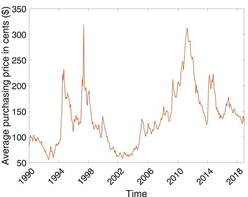
Companies that are operating in global markets have been exposed to swift changes in business conditions due to price volatility in raw materials and commodities. For example, the international coffee market is one of the markets that experience price volatility. Figure 1 presents how procurement prices of a variant of coffee beans, Colombian Milds, evolve over the years between 1990 and 2018. It is discernible in the figure that the bean price fluctuates wildly. Hence, coffee manufacturers that input Colombian Milds into the production need to proactively build strategies to offset the price volatility's impacts on their profits.

Figure 1. Monthly averages of International Coffee Organization prices for Colombian Milds in U.S. cents per lb.

A line graph plotting monthly average prices of Colombian Milds in U.S. cents per lb over 1990 and 2018.

We can witness similar examples in various markets where the firms' operations are fully affected by the volatility observed in commodity prices, such as airline, agriculture, energy, copper, iron, steel, and food. In these industries, companies are exposed to volatile raw material price fluctuations as noted in the studies conducted by Yang and Xia (2009), Berling and Martınez-de Albéniz (2011), Berling and Xie (2014), and Liu and Yang (2015). For example, in the agricultural industry, the arrival of raw materials (i.e. supply process) and demand arrival rate (i.e. demand process) are considered random due to different harvest times and ever-changing weather conditions. Manufacturers operating in this sector usually face a choice between purchasing the current harvested materials and waiting for the materials to be cropped in the next term. If a manufacturer opts to defer the procurement to the next harvest period, she loses the opportunity of procuring the raw material for the current period. Besides, depending on inventory levels of the raw material and the finished product, the manufacturer can manage the demand rate by either elevating the selling price point to sell the finished product at a higher price or decreasing the current price to stimulate the current period demand. Our modeling framework can also be considered as an approximation for the situation that raw material purchase opportunities are always available as the firm requires when the arrival rate of supply flow is sufficiently higher than manufacturing and demand rates. Hence, in our problem framework, the manufacturer (or system operator) can be thought of as a firm operating in the agricultural sector that turns harvested raw materials into a finished product.

Moreover, our modeling framework is applicable for companies that encounter fluctuations in oil prices and exchange rates due to replenishment operations from abroad. As presented in the study of Bailey (2007), airlines companies exercise long-term contracts as a hedge against varying oil prices. Berling and Xie (2014) present an example that depicts how exchange rates can vary. After the spot rate of the euro against the dollar gained a value of over 33% between the years 2006 and 2008, it immediately depreciated its value around 28%, followed by an observable incline in its value of about 20% relative to its previous position. Besides, as provided in the study of Berling and Martınez-de Albéniz (2011), companies in the chemical and food industries, respectively, such as BASF and Nestle, are, too, exposed to price fluctuations in their operations. Hence, in the face of a gloomy outlook for the price volatility in a wide variety of markets ranging from food to energy, companies pursue various operational strategies to alleviate the negative impact of plunge and surge of the procurement prices, which eventually affects the total costs of procurement and manufacturing, as well as the matching rate of demand with supply. For instance, Hewlett-Packard, an American multinational information technology company, dynamically sets its products' selling prices based on the changing conditions to reduce the risk associated with demand uncertainty and procurement cost (Nagali et al. 2008).

The uncertainties that loom over demand and supply sides amplify the need for an approach dealing with these risks on the two sides. A viable method to tackle both sides' challenges is considering procurement, manufacturing, and pricing operations in an integrated manner. This study focuses on the profit implications of managing procurement, manufacturing, and pricing decisions of a manufacturer operating in the presence of a randomly changing environment. Specifically, the model we present in this study aims to shed light on a profit-maximising manufacturer's decisions in a setting where procurement prices of raw materials and the market demand for the finished goods randomly fluctuate. In this context, we are addressing three different research questions: (i) What are the optimal procurement, manufacturing, and pricing strategies for a make-to-stock production system subjected to random environmental changes? (ii) Under which circumstances does dynamic-pricing enhance the expected total profit in the presence of random environmental changes? (iii) What are the effects of production rate, holding cost, procurement price and demand variabilities, customers' price sensitivity, and interaction between supply and demand processes on the system's performance measures?

To tackle these research questions, we consider a make-to-stock production system in the presence of random environmental changes evolving based on a continuous-time Markov process whose state-space is finite and discrete. We formulate the system as an infinite-horizon Markov decision process to maximise the long-run expected profit, and we derive the structural properties of the optimal pricing, manufacturing, and procurement strategies. In particular, we establish that the optimal pricing policy is of state-dependent type in the case of a linear demand. Besides, we present a linear programming formulation of the problem to numerically examine the impact of the system's attributes on the average profit and the optimal procurement, manufacturing, and pricing policies.

The Markovian assumption that we consider accommodates firms to make estimations about future price points, a typical situation for a firm that manages its operations based on a trajectory of the procurement price over time (Yang and Xia 2009; Liu and Yang 2015). With this assumption, the firms can build their purchasing activities both on immediate returns and the long-term implications of future price swings. Hence, in our problem setting, the Markovian framework enables us to include the observation that purchasing price processes are viewed as random by the firms but have trends in the long term and capture a manufacturing firm's ability to make predictions about the price process.

The computational results provide several managerial insights on the expected long-run profit of a make-to-stock production system operating in a randomly fluctuating environment where variation exists on both supply and demand processes. Our computational study suggests that observing a degree of positive correlation among supply and demand processes and high procurement price variation in the presence of a market that comprises customers with low price sensitivity increases the system's expected long-run profit, helping pave the way to increase profit-margin per finished good. Conversely, in the case of a lower production capacity, the system's expected profit relatively falls when supply and demand processes are negatively correlated and holding cost is high as lacking an opportunity to buy raw materials at a lower price and offer them to the market at a higher price.

The findings that we achieve in this study also illustrate how profit improvement with the dynamic pricing policy that the manufacturer could potentially generate can vary in system conditions. In particular, we observe that, under certain conditions, dynamically priced finished goods yield a higher profit of up to $15\mathrm{\%}$ than that of the benchmark policy, i.e. choosing a single price point for a finished good regardless of the state of the system. Moreover, the results show that the positive impact of employing dynamic pricing decreases as the correlation between supply and demand processes negatively increases. We also show the impact of confluence of the two parameters, i.e. customer sensitivity and procurement price variability, on the profit enhancement achieved by dynamic pricing. The profit improvement that the manufacturer observes with the dynamic pricing policy significantly increases in a market that consists of customers with relatively low price sensitivity when procurement price variability is high. In the case of low procurement price variability, the profit enhancement of dynamic pricing remains limited, regardless of the price sensitivity of customers in the market.

Overall, our research contributes to the integrated consideration of manufacturing and dynamic pricing with a random price-dependent demand rate of the finished product and a random raw material flow rate. The results and managerial insights that we derive from our study can be listed as follows:

1. The improvement that dynamic pricing could bring about to the firm's expected profit is highly dependent on the relationship between supply and demand processes, which is also moderated by the degree of demand variability. When there exists a degree of positive correlation between supply and demand processes (i.e. the raw material flow and demand arrival rates are in the form of either high and high or low and low, respectively) and variability in demand is not sufficiently high, dynamically pricing the finished product enhances the expected profit achieved by the firm. Otherwise, the profit improvement that dynamic pricing could bring about remains limited in the case of sufficiently high variation in the demand process. When there is a negative correlation between supply and demand processes, the firm could improve the expected long-run profit with dynamic pricing when demand variability is relatively low.

2. Regardless of the correlation between supply and demand processes, our results suggest that the profit enhancements generated by dynamically pricing the finished product become significant when the variation in procurement price is high. The expected profit impact of dynamic pricing, on the other hand, remains limited as the variation in procurement price lowers.

3. The expected profit enhancement performance of dynamic pricing policy varies depending on the production rate at which the firm's facility is running. When the production rate is less than the expected demand rate, dynamic pricing enhances the firm's expected profit by bringing the flexibility to adjust the price of the finished product based on the inventory level of the final product. When the system observes both limited and excess production capacities evenly, the unit cost of holding one unit of the finished product determines the extent to which dynamic pricing improves the firm's expected profit: the benefit of dynamic pricing is (is not) significant when the unit holding cost is low (high). When the firm owns a sufficient level of production capacity, the profit enhancement capability of dynamic pricing decreases.

We believe these findings help pave the way for the broader implementation of dynamic pricing together with procurement and manufacturing strategies for practitioners in a setting where supply and demand processes fluctuate randomly. In particular, our results shed light on the impact of procurement price variability, demand variability, and the correlation of supply and demand processes on profit enhancement a firm that follows the make-to-stock strategy could achieve with dynamic pricing. We contribute to the relevant literature by demonstrating that the benefit of employing dynamic pricing depends on the variation in procurement price and demand and the correlation between supply and demand processes.

This paper is organised as follows. In the next section, we provide a review of the literature and contextualise our contributions. In Section 3, we describe our setting and present structural analyses of the model, and discuss these results. Section 4 presents an extensive numerical study and discusses the results of our findings. In Section 5, we provide a discussion on our study's key findings, followed by a discussion of future research directions.

2. Literature review

Our work jointly addresses procurement, production, and pricing problems of a manufacturer amid uncertainties on the supply and demand side. Therefore, this study mainly contributes to two streams of literature: (1) procurement/inventory management of a single product in the presence of uncertainties in either supply, demand, or both processes when the market governs the sale price and (2) joint production and pricing decisions of a single product in the presence of uncertainties in either supply, demand, or both processes.

The first stream of literature studies how a firm operating in a production supply chain can execute the optimal procurement/inventory management of a product when uncertainties exist in either supply or demand side; or both sides and the sale prices for the finished goods are driven by the market. In this line of literature, a base-stock policy is proven to be optimal in the absence of fixed ordering costs. When a fixed ordering cost is present, a cost-dependent $(s,S)$ rule is found to be optimal policy. We refer interested readers to Özekici and Parlar (1999) and Haksöz and Seshadri (2007). Kalymon (1971) studies a single-item, multi-period inventory model where prices of the upcoming periods are driven by a Markovian process and establishes bounds of optimal policies. Gavirneni (2004) considers an inventory control problem of a single item where the fluctuations of the raw materials' price are driven by the changes in the exchange rate, presenting that an order-up to policy is the optimal strategy. Liu and Yang (2015) treat a problem in which a make-to-order firm controls its raw material replenishment quantity and sale price periodically when the available procurement prices in the market randomly fluctuate in a Markovian fashion and show that the optimal purchasing policy is a base-stock type. Moreover, Karabağ and Tan (2019) involve an underlying random framework causing to change environmental conditions and investigate the effect of interaction between the procurement and sale prices on the system whose operating environment is exposed to random changes. This field of literature has been expanding with studies that consider additional features such as varying time-dependent purchasing prices (Arnold, Minner, and Eidam 2009), partially observable Markov-modulated demand and supply processes (Arifoğlu and Özekici 2010), implementations of data-driven/real-time procurement strategies (Dai et al. 2020; Zhang, Chan, and Xu 2022; Wang et al. 2022), collaborative procurement opportunities (Karabağ and Tan 2018; Rezaei et al. 2020; Xu et al. 2021), and implementations of different procurement strategies under supply chain disruptions (He, Huang, and Yuan 2016; Li, He, and Minner 2021; Saputro, Figueira, and Almada-Lobo 2021; Corominas 2022; Ardolino et al. 2022).

The second stream of literature focuses on joint production and pricing decisions of a single product when the firm observes uncertainties in either supply or demand side; or both sides. An early seminal work by Li (1988) focuses on a make-to-stock, lost-sale production system, where cumulative production and cumulative sales are represented as Poisson processes with controllable intensities. The production and holding costs are considered to be linear. The author formulates the problem as a continuous-time dynamic programming model under the discounted profit criterion. The linear cost structure makes the analysis tractable, allowing the author to derive analytical results on the optimal inventory and pricing policies. Chen, Feng, and Ou (2006) extend the analysis conducted in the study of Li (1988) by considering backlogs and two different levels of retail prices. Xu and Chao (2009) study the same problem, presented in the work of Chen, Feng, and Ou (2006), with a non-linear holding cost structure under the average cost criterion. The authors further present an efficient bisection algorithm to solve the problem numerically. Chen, Feng, and Ou (2009) broaden the scope of the framework presented in the study of Chen, Feng, and Ou (2006) by analyzing the optimal pricing strategies for a make-to-stock system operating in a batch production mode. The authors consider exponential processing times, which possess the memoryless property and relatively facilitates the analysis. Gayon et al. (2009) analyze a make-to-stock production system with price-sensitive market demand and they focus on only uncertainty emerging in the demand side of the production system. They study the revenue implications of different pricing strategies together with the optimal replenishment policies under each pricing policy. Elhafsi and Hamouda (2018) examine a similar problem to that of Gayon et al. (2009). They extend the market structure into two demand classes and incorporate the inventory allocation decision into the problem framework in addition to decisions studied in Gayon et al. (2009). Allon and Zeevi (2011) deal with the simultaneous determination of pricing, production, and capacity investment decisions by a monopolist firm in a multi-period setting. By employing a Stackelberg game-theoretic approach, Fan et al. (2013) examine a dynamic pricing and production planning problem for a system operating in a competitive market. Shi et al. (2014) develop a joint pricing and production policy for a manufacturing system subject to uncertain machine failures.

The third stream of literature also embraces studies that consider joint pricing and manufacturing decisions in a make-to-order environment. Biller, Muriel, and Zhang (2006) analyze the impact of pricing the product after capacity and flexible investment decisions are made and conclude that price postponement policy potentially enhances the profit between $6\mathrm{\%}$ and $10\mathrm{\%}$. Spengler, Rehkopf, and Volling (2007) study the impact of a revenue management approach built on a bid-price policy. They validate the effectiveness of the proposed policy using the production data of a German steel maker. Hintsches et al. (2010) present a case study of applying revenue management technique based on a bid-price policy in a make-to-order steel manufacturing company. They develop a randomised linear programming-based approach to determine bid prices and conclude that the proposed bid-price policy increases the contribution margin to $13\mathrm{\%}$. Volling et al. (2012) develop a two-stage bid-price control mechanism in the presence of stochastic demand. They find that the proposed approach dominates the results achieved via revenue management methods such as randomised linear programming. Chen, Tai, and Yang (2014) study a production system that is capable of producing two product types: the first one is a type of make-to-order product and the second one is a type of make-to-stock product. The authors analytically characterise the integrated optimal production and pricing policy that considers these two products together, and, numerically show that this integrated policy outperforms the policy of managing these two products individually. Furthermore, studies have been expanding by considering integrated production control and/or inventory allocation decisions in various system configurations such as tandem lines (Veatch and Wein 1994; Millhiser and Burnetas 2013; Xu, Serrano, and Lin 2017), assemble-to-order (ElHafsi, Camus, and Craye 2008; ElHafsi 2009; Benjaafar et al. 2011; Nadar, Akan, and Scheller-Wolf 2014), and make-to-order (Carr and Duenyas 2000; Öner-Közen and Minner 2018).

Among the studies in the relevant literature, the works developed by Gayon et al. (2009) and Karabağ and Tan (2019) are the closest to our research with the problem framework they provide. We first address two significant features that distinguish our work from the studies developed by Gayon et al. (2009) and Karabağ and Tan (2019). Gayon et al. (2009) assume the procurement process is deterministic and study the profit implications of various pricing strategies. They also provide structural results regarding optimal replenishment policies. On the other hand, Karabağ and Tan (2019) do not determine price points of the finished product and suppose the sale price process is given. They focus their attention on developing the optimal procurement and manufacturing strategies. They particularly examine the profit impact of optimal procurement and manufacturing policies in the presence of fluctuating and correlated procurement and sale prices. They assume that procurement and sale prices are driven by the market, which is governed by a continuous-time Markov process. Furthermore, they present a characterisation of the optimal procurement and manufacturing strategies. Table 1 summarises a comparison of our work and studies conducted by Gayon et al. (2009) and Karabağ and Tan (2019) in terms of operational decisions under consideration and supply, manufacturing, and demand processes, and whether it considers a correlation relationship between these processes.

Table 1. A Comparison of Gayon et al. (2009), Karabağ and Tan (2019), and This Study.

Study	Decisions	Supply process	Production process	Demand process	Correlation between demand and supply processes
Gayon et al. (2009)	Production, pricing	Not considered	Random, capacitated	Random, price-sensitive	×
Karabağ and Tan (2019)	Procurement, production	Random	Random, capacitated	Random, governed by the market	×
This study	Procurement, production, pricing	Random	Random, capacitated	Random, price-sensitive	$✓$

To the best of our knowledge, our study is the first to fuse a monopolist manufacturing firm's procurement, manufacturing, and pricing strategies simultaneously. Moreover, this study is the first to incorporate the correlation relationship between supply and demand processes into the firm's optimisation problem and analyze how such a relationship affects procurement, manufacturing, and pricing decisions. We also quantify the profit implications of this correlation relationship in our problem framework.

Our study mainly contributes to the relevant literature by analyzing the value of using dynamic pricing policy and its interaction between supply and demand processes, evolving according to a Markov process, in a make-to-stock system that fluctuates across different environments. Besides, we derive analytical results that provide structural properties of the optimal procurement, manufacturing, and pricing decisions. Finally, we develop a linear programming formulation to study the effects of system characteristics on the firm's optimal decisions.

3. Mathematical model

In this section, we first introduce the problem framework and then present a dynamic programming formulation for the problem. Furthermore, we establish the optimal control strategies for procurement, manufacturing, and pricing decisions and characterise their structural properties. Lastly, we present a linear programming formulation to numerically obtain the optimal procurement, manufacturing, and pricing decisions of the system.

3.1. Problem framework

We consider a make-to-stock system with a single manufacturing facility that produces to satisfy the demand of a single item. The graphical illustration of the system is portrayed in Figure 2.

Figure 2. Problem illustration.

Graphical description of the system we focus on in this study, which includes a single manufacturing facility operating in a fluctuating environment with two buffers and exponentially distributed production and raw material times.

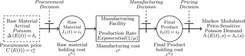
The manufacturing system is operating in an environment that is exposed to random exogenous economic changes. We can represent these changes by a finite number of F different states, i.e. at any given time t, the environment state, which we denote by $E\left(t\right)$, can be in one of these states. The system operator (or manufacturer) is able to directly observe the environment state at any time t, i.e. $E\left(t\right)\in \mathbb{F}=\{1,2,\dots ,F\}$. Although these environmental changes directly affect the system's supply and demand processes, and its procurement prices, the system operator can neither intervene in nor alter these changes by her decisions.

The environmental changes are driven by a homogeneous continuous-time Markov chain that possesses a transition rate matrix R. In the transition matrix, the element $r_{kl}$ describes the rate leaving from state k and entering state $l\ne k$ where $k,l\in \mathbb{F}$. In order to avoid any possible technical issues, this Markov chain is considered to be recurrent.

The system operator keeps two different forms of inventory to perform her operations as raw material and final product, corresponding to the first and second inventory levels, respectively. She is able to directly observe the first and second inventory levels at any time t, i.e. $I_1\left(t\right)$ and $I_2\left(t\right)$ where $I_1\left(t\right),I_2\left(t\right)\in \mathbb{Z}=\{0,1,2,\dots \}$. The costs of keeping one unit of stock in the first and second inventory are $c^{h_1}$ and $c^{h_2}$, respectively.

Given that the system operator fully observes inventory levels and environment states, she attempts to determine the optimal procurement, manufacturing, and pricing strategies that maximise her average profit over an infinite planning horizon. The system details are given in the subsequent sections.

3.1.1. Procurement process

The raw materials arrive at the system according to a Markov-modulated Poisson process whose rate is only a function of the environment state. That is, the raw material inter-arrival times are exponentially distributed with the rates depending on the environment states. For environment state $E\left(t\right)=e\in \mathbb{F}$, the raw material flow rate is $\mathrm{\Delta }\left(E\right(t\left)\right)={\delta }_e$ where ${\delta }_e\in \mathbb{U}$=$\{{\delta }_1,{\delta }_2,\dots ,{\delta }_F\}$.

Each time a raw material unit arrives at the system, the system operator takes a decision on whether to buy it. If the system operator buys one unit of the arriving raw material, she is charged the procurement price available in the current environment and adds that unit to her raw material inventory. Otherwise, she loses the chance of buying this particular raw material unit without any immediate penalty cost. The procurement price varies depending on the environment state; that is, for environment $E\left(t\right)=e\in \mathbb{F}$, the procurement price is $C\left(E\right(t\left)\right)$=$c_e^g$ where $c_e^g\in \mathbb{G}$=$\{c_1,c_2,\dots ,c_F\}$.

3.1.2. Production process

With the system operator's manufacturing decision, a raw material unit is released into the production system. The system is capable of processing a single item at a time, i.e. it has a limited production capacity. The processing time follows an exponential distribution with a mean value of μ. The system operator pays a production cost of $c^p$ to process one unit of raw material. After being processed, each item is placed in the second inventory to satisfy the arriving customers' demand.

3.1.3. Demand process

The customers arrive at the system according to a Markov-modulated Poisson process whose rate is a function of both system's sale price and environment state. Each arriving customer requests only a single unit of the final product, and it is met as long as the second inventory is non-empty. When there exists no stock unit in the second inventory, the system operator does not necessarily need to decide on the sale price, (see, e.g. Gallego and Van Ryzin 1994; Gayon and Dallery 2007; Gayon et al. 2009, for other studies that make a similar assumption). A demand that cannot be met from the stock immediately is lost without any penalty.

The system operator employs a dynamic pricing strategy to set her unit sale price. That is, at any given time t, the sale price is a function of environment state $E\left(t\right)=e$ where $e\in \mathbb{F}$ and stock levels $I_1\left(t\right)=i_1$ and $I_2\left(t\right)=i_2$ where $i_1,i_2\in \mathbb{Z}$. We denote the sale price when environment state is e and stock levels are $i_1$ and $i_2$ by $s(e,i_1,i_2)$. Correspondingly, for any given states of e, $i_1$, and $i_2$, the demand arrival rate is $\mathrm{\Lambda }\left(s\right(e,i_1,i_2\left)\right)={\lambda }_e\left(s\right(e,i_1,i_2\left)\right)$ where ${\lambda }_e\left(s\right(e,i_1,i_2\left)\right)\in \mathbb{K}$=$\left\{{\lambda }_1\right(s(e,i_1,i_2)),{\lambda }_2(s(e,i_1,i_2)),\dots ,{\lambda }_F(s(e,i_1,i_2)\left)\right\}$. In each environment, the demand rate is bounded by ${\mathrm{\Lambda }}_e$, i.e. ${\lambda }_e\left(s\right(e,i_1,i_2\left)\right)\le {\mathrm{\Lambda }}_e$ where $e\in \mathbb{F}$ and $i_1,i_2\in \mathbb{Z}$. This reasonable assumption is necessary to uniformise the Markov decision process. On the other hand, for any given environment state e and inventory levels $i_1$ and $i_2$, we assume that there is a one-to-one correspondence between the sale price and the demand arrival rate and that the rate is a decreasing function of the sale price. The set of allowable prices is identical for all $(e,i_1,i_2)$ where $e\in \mathbb{F}$ and $i_1,i_2\in \mathbb{Z}$. It is denoted by ${\mathcal{D}}^{\mathrm{\prime }}=\mathcal{D}\cup \left\{0\right\}$ where $\mathcal{D}$ is a compact subset of the set of non-negative real numbers ${\mathbb{R}}^{+}$.

Lastly, we consider that the revenue rate ${\omega }_e\left(s\right(e,i_1,i_2\left)\right)=s(e,i_1,i_2){\lambda }_e\left(s\right(e,i_1,i_2\left)\right)$ is a continuous and bounded function. For a given state $(e,i_1,i_2)$, the revenue rate is also a concave function in sale price, which stems from the standard economic assumption that the marginal revenue is decreasing in output (Gayon et al. 2009).

3.2. Optimal control model

The system is memory-less since the time elapsed between each transition in the system evolves according to an exponential distribution. Therefore, we can restrict our decision epochs only to the times when the state changes happen (Karabağ and Tan 2019). This fact makes it possible to represent our problem as a Markov decision process whose optimal solution belongs to the class of stationary policies and the system through time-independent state variables (Puterman 2014).

Therefore, we can define the state of the system as $(e,\underset{\_}{i})$ where $(e,\underset{\_}{i})\in \mathbb{F}\times {\mathbb{Z}}^2$. In this state variable, e and $\underset{\_}{i}$ respectively denote the environment state and the first and second inventory levels. For each state $(e,\underset{\_}{i})$, the system operator makes decisions of procurement, manufacturing, and pricing. The operator's procurement and manufacturing decisions are denoted by $d_g(e,\underset{\_}{i})\in {\mathbb{D}}_g=\{0,1\}$ and $d_p(e,\underset{\_}{i})\in {\mathbb{D}}_p=\{0,1\}$, respectively. In case of taking a procurement action, i.e. $d_g(e,\underset{\_}{i})$=1, when the environment state is e, the system operator pays a unit procurement cost $c_e^g$; otherwise, she pays nothing. On the other hand, in case of taking a manufacturing action, i.e. $d_p(e,\underset{\_}{i})$=1, she pays a unit production cost $c^p$, regardless of the environment state. When there is no production, i.e. $d_p(e,\underset{\_}{i})$=0, there will be no cost that she needs to pay. The operator's sale price decision is denoted by $d_z(e,\underset{\_}{i})$ where $d_z(e,\underset{\_}{i})\in {\mathcal{D}}^{\mathrm{\prime }}$. When an action $d_z(e,\underset{\_}{i})=s$ is taken, she gets a revenue of s from selling one unit of the final product.

Let $\ell$ be a policy that prescribes the action $d^{\ell }(e,\underset{\_}{i})=\left(d_g\right(e,\underset{\_}{i}),d_p(e,\underset{\_}{i}),d_z(e,\underset{\_}{i}\left)\right)$ for each system state $(e,\underset{\_}{i})$ and $(e^{\mathrm{\prime }},\underset{\_}{i^{\mathrm{\prime }}})$ be the initial state of the system. For given $\ell$ and $(e^{\mathrm{\prime }},\underset{\_}{i^{\mathrm{\prime }}})$, we can define the system's expected profit per unit time over an infinite planning horizon as follows: (1) $\begin{array}{rl}& {\varphi }^{\ell }(e^{\mathrm{\prime }},\underset{\_}{i^{\mathrm{\prime }}})\\ & =\underset{T\to \mathrm{\infty }}{lim}\frac{{\mathrm{E}}_{(e^{\mathrm{\prime }},\underset{\_}{i^{\mathrm{\prime }}})}^{\ell }\left[\begin{array}{c}{\displaystyle {\int }_0^{T}S\left(E\right(t),I_1(t),I_2(t\left)\right)\mathrm{d}{N}_Z\left(t\right)}\\ {\displaystyle -{\int }_0^{T}C\left(E\right(t\left)\right)\mathrm{d}{N}_G\left(t\right)}\\ {\displaystyle -{\int }_0^T\left(c^{h_1}{I}_1\right(t)+c^{h_2}{I}_2(t\left)\right)\mathrm{d}t}\\ {\displaystyle -{\int }_0^T{c}^p\mathrm{d}{N}_P\left(t\right)}\end{array}\right]}{T},\end{array}$(1) where $N_Z\left(t\right)$ is the total number of customers whose requests are met until time t, $N_G\left(t\right)$ represents the total number of units of the raw material procured until time t, and $N_P\left(t\right)$ denotes the total number of units of the final product manufactured until time t. The goal of the system operator is to determine a policy ${\ell }^{\ast }$ that satisfies (2) $\begin{array}{r}{\varphi }^{\ast }(e,\underset{\_}{i})=\underset{\ell }{sup}{\varphi }^{\ell }(e,\underset{\_}{i})\end{array}$(2) for all states.

Given that the time elapsed between each transition is always exponentially distributed and the maximum transition rate is finite, it is possible to construct a discrete-time equivalent of the system through the standard uniformisation and normalisation techniques (Lippman 1975; Serfozo 1979). As a uniform transition rate, we choose (3) $\begin{array}{r}\psi =\sum _{e\in \mathbb{F}}\sum _{f\in \mathbb{F}\setminus \left\{e\right\}}{r}_{ef}+\sum _{e\in \mathbb{F}}{\delta }_e+\sum _{e\in \mathbb{F}}{\mathrm{\Lambda }}_e+\mu ,\end{array}$(3) in our problem and, without loss of generality, we normalise it to 1, i.e. $\psi =1$. Indeed, this allows us to observe the system at exponentially distributed time intervals with a mean of 1. After applying both uniformisation and normalisation techniques to our problem together with the chosen ψ, the optimality equation of the system is defined as follows: (4) $\begin{array}{rl}\varphi (e,\underset{\_}{i})+q^{\ast }& =V_g\varphi (e,\underset{\_}{i})+V_p\varphi (e,\underset{\_}{i})+V_z\varphi (e,\underset{\_}{i})\\ & +V_f\varphi (e,\underset{\_}{i})-(c^{h_1}{i}_1+c^{h_2}{i}_2),\end{array}$(4) where $q^{\ast }$ is the optimal expected profit and $\varphi (e,\underset{\_}{i})$ the relative gap between the current and the optimal expected profits. Also, for any real function $\theta (e,\underset{\_}{i})$, the operators $V_g\theta (e,\underset{\_}{i})$, $V_p\theta (e,\underset{\_}{i})$, $V_z\theta (e,\underset{\_}{i})$, and $V_f\theta (e,\underset{\_}{i})$ appeared in the optimality equation are described as follows: (5) $\begin{array}{rl}{V}_g\theta (e,\underset{\_}{i})& =max\{{\delta }_e\theta (e,\underset{\_}{i}+u_1)-{\delta }_e{c}_e^g,{\delta }_e\theta (e,\underset{\_}{i})\},\end{array}$(5) (6) $\begin{array}{rl}{V}_p\theta (e,\underset{\_}{i})& =\{\begin{array}{l}max\left\{\mu \right(\theta (e,\underset{\_}{i}-u_1\\ +u_2)-c^p),\mu \theta (e,\underset{\_}{i})\},& i_1>0,\\ \mu \theta (e,\underset{\_}{i}),& i_1=0,\end{array}\end{array}$(6) (7) $\begin{array}{rl}{V}_z\theta (e,\underset{\_}{i})& =\{\begin{array}{l}\underset{s\in {\mathcal{D}}^{\mathrm{\prime }}}{max}\left\{{\omega }_e\right(s)\\ +{\lambda }_e\left(s\right)\theta (e,\underset{\_}{i}-u_2)\\ +({\mathrm{\Lambda }}_e-{\lambda }_e(s\left)\right)\theta (e,\underset{\_}{i})\}& i_2>0,\\ {\mathrm{\Lambda }}_e\theta (e,\underset{\_}{i}),& i_2=0,\end{array}\end{array}$(7) (8) $\begin{array}{rl}{V}_f\theta (e,\underset{\_}{i})& =(\sum _{l\in \mathbb{F}\setminus \left\{k\right\}}{\delta }_l+\sum _{l\in \mathbb{F}\setminus \left\{k\right\}}{\mathrm{\Lambda }}_l+\sum _{l\in \mathbb{F}\setminus \left\{k\right\}}\sum _{m\ne l}{r}_{lm})\\ & \times \theta (e,\underset{\_}{i})+\sum _{l\in \mathbb{F}\setminus \left\{k\right\}}{r}_{kl}\theta (l,\underset{\_}{i}),\end{array}$(8) where $u_1$ and $u_2$ are respectively the unit vectors in the direction of $i_1$ and $i_2$; that is, $u_1$=(1, 0) and $u_2$=(0, 1). $V_g\theta (e,\underset{\_}{i})$ and $V_p\theta (e,\underset{\_}{i})$ correspond to the procurement and manufacturing decisions in the system, respectively. Furthermore, $V_f\theta (e,\underset{\_}{i})$ represents both fictitious and environmental transitions in the system. Lastly, $V_z\theta (e,\underset{\_}{i})$ denotes the system operator's sale price decision.

The model satisfies the standard conditions given in Puterman (2014), which establishes the existence of an optimal deterministic stationary policy and the convergence of the optimal solution. With this fact, we can be sure that, for our model, the Bellman equation ${\varphi }^{\ast }+q^{\ast }=V{q}^{\ast }$ holds and that there is a unique solution of $q^{\ast }$.

3.3. Structural results

We utilise the event-based dynamic programming approach provided by Koole (1998) for characterising the structural properties of the optimal control strategies. As you can notice in Equation (4(4) $\begin{array}{rl}\varphi (e,\underset{\_}{i})+q^{\ast }& =V_g\varphi (e,\underset{\_}{i})+V_p\varphi (e,\underset{\_}{i})+V_z\varphi (e,\underset{\_}{i})\\ & +V_f\varphi (e,\underset{\_}{i})-(c^{h_1}{i}_1+c^{h_2}{i}_2),\end{array}$(4) ), we associate each event in the system with a particular operator function, i.e. the procurement, manufacturing, pricing, and fictitious transition operators. Indeed, this approach allows us to examine the propagation of the value function properties through the propagation properties of the event operators (Karabağ and Tan 2019). More specifically, if a structural property holds under a set of given assumptions for all event operators, the same property is also preserved by the value function being constructed with these operators.

In Theorems 3.1 and 3.2, using these standard arguments related to the event-based dynamic programming framework together with the findings in Koole (1998), we establish the optimality of a state-dependent threshold policy for the system's procurement and manufacturing decisions, respectively.

Theorem 3.1

The optimal procurement policy is a state-dependent threshold policy. Specifically, for any given state $(e,i_1,i_2)$, there exists a threshold level $X_g^{\ast }(e,i_2)$ such that (9) $\begin{array}{r}{X}_g^{\ast }(e,i_2)=\arg \underset{i_1}{min}\{(e,i_1,i_2)|d_g^{\ast }(e,i_1,i_2)=0\}\end{array}$(9) where $d_g^{\ast }(\cdot )$ denotes the optimal procurement decision for any state given as an input. Correspondingly, for any given state $(e,i_1,i_2)$, it is optimal to procure if $i_1<X_g^{\ast }(e,i_2)$; otherwise, it is optimal not to procure.

Theorem 3.2

The optimal manufacturing policy is a state-dependent threshold policy. Specifically, for any given state $(e,i_1,i_2)$ where $i_1+i_2=k$, there exists a threshold level $X_p^{\ast }(e,i_2)$ such that (10) $\begin{array}{rl}{X}_p^{\ast }(e,i_2)& =\arg \underset{i_1}{max}\{(e,i_1,k-i_1)|\\ & d_p^{\ast }(e,i_1,k-i_1)=0\}.\end{array}$(10) where $d_p^{\ast }(\cdot )$ denotes the optimal manufacturing decision for any state given as an input. Correspondingly, for any given state $(e,i_1,i_2)$ where $i_1+i_2=k$, it is optimal to manufacture if $i_1>X_p^{\ast }(e,i_2)$; otherwise, it is optimal not to manufacture.

Also, Theorems 3.3 and 3.4 present the monotonicity properties of the optimum threshold policies that we have provided in Theorems 3.1 and 3.2.

Theorem 3.3

$X_g^{\ast }(e,i_2)$ is non-ascending with respect to both raw material inventory level $i_1$ and final product inventory level $i_2$.

Let $X_g^{\ast }(e,i_2)$ and $X_g(e,i_2^{\mathrm{\prime }})$ be the threshold levels for the procurement decisions in states $(e,i_1,i_2)$ and $(e,i_1,i_2^{\mathrm{\prime }})$ where $i_2^{\mathrm{\prime }}>i_2$. Theorem 3.3 refers that $X_g^{\ast }(e,i_2)\ge X_g(e,i_2^{\mathrm{\prime }})$. Analogously, it can also be shown that the corresponding threshold levels have a non-ascending order in the raw material inventory levels. Let $X_g^{\ast }(e,i_2)$ and $X_g(e,i_2)$ be the threshold levels for the procurement decisions in states $(e,i_1,i_2)$ and $(e,i_1^{\mathrm{\prime }},i_2)$ where $i_1^{\mathrm{\prime }}>i_1$. Theorem 3.3 implies that for these two states, the corresponding threshold levels satisfy $X_g^{\ast }(e,i_2)\ge X_g(e,i_2)$. Intuitively, Theorem 3.3 indicates that as the finished goods and raw material stock levels increase, the threshold that triggers the system to accept raw materials becomes more restrictive. When there exist sufficiently high stock in both raw material and finished goods inventory, purchasing more raw materials by lowering the corresponding threshold will lead to an increase in the manufacturer's holding cost rather than bring a benefit to her. So, the manufacturer will incline not to reduce the threshold level as the stock levels are increasing.

Theorem 3.4

$X_p^{\ast }(e,i_2)$ is non-descending with respect to the raw material inventory level $i_1$ and non-ascending with respect to the final product inventory level $i_2$.

Let $X_p^{\ast }(e,i_2)$ and $X_p(e,{\hat{i}}_2)$ be the threshold levels of the manufacturing decisions in states $(e,i_1,i_2)$ and $(e,i_1,{\hat{i}}_2)$ where ${\hat{i}}_2>i_2$. Theorem 3.4 implies that $X_p^{\ast }(e,i_2)\ge X_p(e,{\hat{i}}_2)$. Similarly, it can also be shown that the corresponding threshold levels have a non-descending order in the raw material inventory levels. Let $X_p^{\ast }(e,i_2)$ and $X_p(e,i_2)$ be the threshold levels of the manufacturing decisions in states $(e,i_1,i_2)$ and $(e,{\hat{i}}_1,i_2)$ where ${\hat{i}}_1>i_1$. Theorem 3.4 states that the manufacturing threshold levels belonging to these two states satisfy $X_p^{\ast }(e,i_2)\le X_p(e,i_2)$. Intuitively, Theorem 3.4 demonstrates that as the finished goods (raw material) stock level increases, the production threshold level becomes more (less) restrictive. Let's suppose that the manufacturer has a high number of units in her raw material inventory. In such a case, she will be able to convert the excessive amount stock to finished goods and sell it at a reasonable price as soon as possible. Otherwise, she may need to keep it in her inventory for a while thereby increasing her holding cost. Considering this fact, she will lower the production threshold as the raw material stock level increases. On the other hand, in the case of having a large number of units in the finished goods inventory, producing more products by lowering the corresponding threshold level will lead to an increase in the manufacturer's holding cost. So, the manufacturer will incline not to reduce the production threshold level as the stock level in the finished goods inventory increases.

Moreover, we find that the optimal sale price of the final product declines as the raw material and final product inventory increase. We present our findings in Theorems 3.5 and 3.6.

Theorem 3.5

Let $i_2<i_2^{\mathrm{\prime }}$ and $s^{\ast }$ and ${s^{\ast }}^{\mathrm{\prime }}$ be the optimal sale prices for states $(e,i_1,i_2)$ and $(e,i_1,i_2^{\mathrm{\prime }})$, respectively. Then, the sequence of the corresponding optimal prices is $s^{\ast }\ge {s^{\ast }}^{\mathrm{\prime }}$.

Theorem 3.6

Let $i_1<i_1^{\mathrm{\prime }}$ and $s^{\ast }$ and ${s^{\ast }}^{\mathrm{\prime }}$ be the optimal sale prices for states $(e,i_1,i_2)$ and $(e,i_1^{\mathrm{\prime }},i_2)$, respectively. Then, the sequence of the corresponding optimal prices is $s^{\ast }\ge {s^{\ast }}^{\mathrm{\prime }}$.

With an increase in the inventory levels, the potential holding cost for the system will also increase. In such a case, the system operator will intend to sell final products faster, resulting in a decrease in the prices charged. Theorems 3.5 and 3.6 confirm that these intuitions hold for the optimal pricing strategies. As a result, we can conclude that as the stock levels of either raw materials or finished goods in the system increase, the optimal price decreases.

Theorem 3.7

If $s^{\ast }$ is the unique price that maximises the revenue function ${\omega }_e(\cdot )$ and the optimal price corresponding to state $(e,i_1,i_2^{\ast })$, then, for any given state $(e,i_1,i_2)$, (11) $\begin{array}{r}{d}_z^{\ast }(e,i_1,i_2)=\{\begin{array}{ll}s(e,i_1,i_2)\ge s^{\ast },& \mathrm{i}\mathrm{f}{i}_2\le i_2^{\ast },\\ s(e,i_1,i_2)\le s^{\ast },& \mathrm{i}\mathrm{f}{i}_2>i_2^{\ast }.\end{array}\end{array}$(11)

Theorem 3.8

If $s^{\ast }$ is the unique price that maximises the revenue function ${\omega }_e(\cdot )$ and the optimal price corresponding to state $(e,i_1^{\ast },i_2)$, then, for any given state $(e,i_1,i_2)$, (12) $\begin{array}{r}{d}_z^{\ast }(e,i_1,i_2)=\{\begin{array}{ll}s(e,i_1,i_2)\ge s^{\ast },& \mathrm{i}\mathrm{f}{i}_1\le i_1^{\ast },\\ s(e,i_1,i_2)\le s^{\ast },& \mathrm{i}\mathrm{f}{i}_1>i_1^{\ast }.\end{array}\end{array}$(12)

Suppose that there exists a sale price that maximises the revenue function ${\omega }_e(\cdot )$ and that it is the optimal price corresponding to $(e,i_1^{\ast },i_2)$. In such a case, it can also be interpreted as the optimal price for the deterministic equivalent of the problem we consider in this study, where there is no need to carry any inventory (Federgruen and Heching 1999; Gayon and Dallery 2007). Accordingly, Theorems 3.7 and 3.8 mean that in case of the existence of such a sale price, a price discount with respect to the optimal deterministic price, $s^{\ast }$ is offered whenever the first and second inventory levels are above a certain threshold.

Lastly, we prove the existence of a state-dependent solution for the optimal pricing policy when the demand arrival rate function has a linear form. Theorem 3.9 presents the details of our findings. The findings that are given in Theorem 3.9 overlap that of Gayon et al. (2009) as they consider the same form of demand structure in a very similar operating environment.

Theorem 3.9

Let ${\mathrm{\Lambda }}_e(1-\text{β}s)$ be the demand rate function for environment state $e\in \mathbb{F}$. In such a case, the optimal sale price can be expressed as follows: (13) $\begin{array}{rl}& d_z^{\ast }(e,i_1,i_2)\\ & =\{\begin{array}{ll}0,& \begin{array}{l}\text{β}\left(\varphi \right(e,\underset{\_}{i})\\ -\varphi (e,\underset{\_}{i}-u_2))<-1,\end{array}\\ {\displaystyle \frac{\begin{array}{l}1+\text{β}\left(\varphi \right(e,\underset{\_}{i})\\ -\varphi (e,\underset{\_}{i}-u_2))\end{array}}{2\text{β}}},& \begin{array}{l}|\text{β}\left(\varphi \right(e,\underset{\_}{i})\\ -\varphi (e,\underset{\_}{i}-u_2))|\le 1,\end{array}\\ {\displaystyle \frac{1}{\text{β}}},& \begin{array}{l}\text{β}\left(\varphi \right(e,\underset{\_}{i})\\ -\varphi (e,\underset{\_}{i}-u_2))>1.\end{array}\end{array}\end{array}$(13)

In the first part of Theorem 3.9, the system operator sets the price level to zero, and, in turn, the demand arrival rate reaches its maximum. In the case of a significantly high amount of stock in her inventory, the system operator may need to incur very high inventory holding cost and the price levels that she can utilise may not be sufficient to compensate these costs. When the marginal value of having one additional unit of the finished product is less than -1/β, the system operator attempts to decrease high amount of inventory levels by implementing the policy given in the first part. In the second part of Theorem 3.9, the marginal value of keeping one additional unit of the finished product is between $-1/\text{β}$ and $1/\text{β}$, corresponding to the cases in which the the system operator utilises pricing as a lever for profit maximisation, i.e. she sets her sale price to a level between 0 and $1/\text{β}$ when the value function satisfies the corresponding condition. The last part of Theorem 3.9 corresponds to the case where the marginal value of having one additional unit of the finished product is higher than 1/β. In such a case, the system operator will not sell the on-hand stock. Correspondingly, she sets the sale price to its maximum value, $1/\text{β}$, thereby making the demand arrival rate zero. With this pricing strategy, the system operator keeps her stock to sell them in an environment having a higher profit margin. This theorem can also help us to alleviate the computational complexity that we encounter in finding the optimal price by employing the solution algorithms such as value iteration or policy iteration.

3.4. Linear programming formulation

In order to numerically compute the optimal threshold values of the system's procurement and manufacturing decisions and optimal sale price decision, we utilise a linear programming formulation. This solution approach has been previously used in the literature (see, e.g. Kunnumkal and Topaloglu 2010; Diamant, Milner, and Quereshy 2018; Hosseini and Tan 2019; Marquinez et al. 2021). Basically, it enables us to harness the power of the state-of-art optimisation software packages to solve the problem and to compute the steady-state probabilities together with the system's performance measures without an extra effort. In Table 2, we list all of the sets and indices employed in the linear programming formulation.

Table 2. Sets, indices, and parameters considered in the LP formulation.

$d_g$: Procurement decision, $d_g\in {\mathbb{D}}_g=\{0,1\}$	$i_1$: First inventory level, $i_1\in {\mathbb{I}}_1=\{0,1,\dots ,L_1\}$
$d_p$: Manufacturing decision, $d_p\in {\mathbb{D}}_p=\{0,1\}$	$i_2$: Second inventory level, $i_2\in {\mathbb{I}}_2=\{0,1,\dots ,L_2\}$
$d_z$: Sale price decision, $d_z\in \mathbb{D}$	e: Environment state, $e\in \mathbb{F}=\{1,2,\dots ,F\}$
$\underset{\_}{i}$: Inventory levels state, $\underset{\_}{i}\in {\mathbb{J}}^1$	${\mathbb{J}}^1$: $\left\{\right(i_1,i_2\left)\right|i_k\in {\mathbb{I}}_k\mathrm{w}\mathrm{h}\mathrm{e}\mathrm{r}\mathrm{e}k\in \{1,2\}\}$
$\mathbb{D}$: Discretised set of possible prices, $\mathbb{D}\approx {\mathcal{D}}^{\mathrm{\prime }}$	${\mathbb{J}}^2$: $\left\{\right(i_1,i_2\left)\right|i_1\in {\mathbb{I}}_1,i_2\in \left\{0\right\}\}$
${\mathbb{J}}^3$: $\left\{\right(i_1,i_2\left)\right|i_1\in {\mathbb{I}}_1,i_2\in {\mathbb{I}}_2\setminus \left\{0\right\}\}$

In the problem setting given in Section 3.2, there is no restriction on the first and second inventory levels, i.e. they can theoretically go up to infinity. To deal with this issue, we should truncate the inventory levels and use the approach based on this truncated version. To this end, we introduce two new parameters $L_1$ and $L_2$, i.e. they are the truncation levels corresponding to the first and second inventory, respectively. To avoid any numerical errors, both $L_1$ and $L_2$ should be set to a sufficiently high value so that the global optimal solution does not change when we increase one of these variables. As another requirement to employ the linear programming approach, we need to discretise the possible sale price levels that the system operator can choose. With a sufficient grid resolution, the formulation would provide us with a solution that is indeed close to the optimal one. The discretised price set is denoted by $\mathbb{D}$.

With the introduction of the truncation levels, the variables indicating the first and second inventory levels belong to the following sets: $i_1\in {\mathbb{I}}_1=\{0,1,2,\dots ,L_1\}$ and $i_2\in {\mathbb{I}}_2$=$\{0,1,2,\dots ,L_2\}$. Correspondingly, $\underset{\_}{i}$, which denotes the inventory levels of the state variable, pertains to the set ${\mathbb{J}}^1$=$\left\{\right(i_1,i_2\left)\right|i_k\in {\mathbb{I}}_k\mathrm{w}\mathrm{h}\mathrm{e}\mathrm{r}\mathrm{e}k\in \{1,2\}\}$. The decision variables of the LP formulation are denoted by $Y_{e,\underset{\_}{i},d_g,d_p,d_z}$, which can be interpreted as the long-run fraction of the time spent in state $(e,\underset{\_}{i})$ with actions $d_g$, $d_p$, and $d_z$.

With the sets, indices, and decision variables we introduced above, the linear programming formulation of the problem is defined as follows: (14) $\begin{array}{rl}& max\alpha =\sum _{e\in \mathbb{F}}\sum _{\underset{\_}{i}\in {\mathbb{J}}^1}\sum _{d_g\in {\mathbb{D}}_g}\sum _{d_p\in {\mathbb{D}}_p}\sum _{d_z\in \mathbb{D}}{Y}_{e,\underset{\_}{i},d_g,d_p,d_z}\\ & \times \left(d_z{\lambda }_e\right(d_z)-{\delta }_e{d}_g{c}_e^g-\mu d_p{c}^p-i_1{c}^{h_1}-i_2{c}^{h_2}),\end{array}$(14) subject to (15) $\begin{array}{rl}& \sum _{d_g\in {\mathbb{D}}_g}\sum _{d_p\in {\mathbb{D}}_p}(Y_{e,\underset{\_}{i},d_g,d_p,0}-d_g{\delta }_e{Y}_{e,\underset{\_}{i}-u_1,d_g,d_p,0}\\ & -d_p\mu Y_{e,\underset{\_}{i}+u_1-u_2,d_g,d_p,0}-{\lambda }_e\left(d_z\right)Y_{e,\underset{\_}{i}+u_2,d_g,d_p,0}\\ & -\sum _{k\in \mathbb{F}\setminus \left\{l\right\}}{r}_{kl}{Y}_{k,\underset{\_}{i},d_g,d_p,0}\\ & -(1-d_g{\delta }_e-d_p\mu -\sum _{k\in \mathbb{F}\setminus \left\{l\right\}}{r}_{lk})Y_{e,\underset{\_}{i},d_g,d_p,0})=0,\\ & \mathrm{\forall }e\in \mathbb{F},\mathrm{\forall }\underset{\_}{i}\in {\mathbb{J}}^2,\end{array}$(15) (16) $\begin{array}{rl}& \sum _{d_g\in {\mathbb{D}}_g}\sum _{d_p\in {\mathbb{D}}_p}\sum _{d_z\in \mathbb{D}}(Y_{e,\underset{\_}{i},d_g,d_p,d_z}-d_g{\delta }_e{Y}_{e,\underset{\_}{i}-u_1,d_g,d_p,d_z}\\ & -d_p\mu Y_{e,\underset{\_}{i}+u_1-u_2,d_g,d_p,d_z}-{\lambda }_e\left(d_z\right)Y_{e,\underset{\_}{i}+u_2,d_g,d_p,d_z}\\ & -\sum _{k\in \mathbb{F}\setminus \left\{l\right\}}{r}_{kl}{Y}_{k,\underset{\_}{i},d_g,d_p,d_z}-(1-d_g{\delta }_e-d_p\mu -{\lambda }_e(d_z)\phantom{\sum _{k\in \mathbb{F}\setminus \left\{l\right\}}}\\ & -\sum _{k\in \mathbb{F}\setminus \left\{l\right\}}{r}_{lk})Y_{e,\underset{\_}{i},d_g,d_p,d_z})=0,\mathrm{\forall }e\in \mathbb{F},\mathrm{\forall }\underset{\_}{i}\in {\mathbb{J}}^3,\end{array}$(16) (17) $\begin{array}{rl}& \sum _{e\in \mathbb{F}}\sum _{\underset{\_}{i}\in {\mathbb{J}}^1}\sum _{d_g\in {\mathbb{D}}_g}\sum _{d_p\in {\mathbb{D}}_p}\sum _{d_z\in \mathbb{D}}{Y}_{e,\underset{\_}{i},d_g,d_p,d_z}=1,\end{array}$(17) (18) $\begin{array}{rl}& Y_{e,\underset{\_}{i},d_g,d_p,d_z}=0,\\ & \mathrm{\forall }e\in \mathbb{F},\mathrm{\forall }\underset{\_}{i}\in \left\{(i_1,i_2)\right|i_1=0,i_2\in {\mathbb{I}}_2\},\\ & \mathrm{\forall }{d}_g\in {\mathbb{D}}_g,d_p\in \left\{1\right\},\mathrm{\forall }{d}_z\in \mathbb{D},\end{array}$(18) (19) $\begin{array}{rl}& Y_{e,\underset{\_}{i},d_g,d_p,d_z}=0,\\ & \mathrm{\forall }e\in \mathbb{F},\mathrm{\forall }\underset{\_}{i}\in \left\{(i_1,i_2)\right|i_1\in {\mathbb{I}}_1,i_2=0\},\mathrm{\forall }{d}_g\in {\mathbb{D}}_g,\\ & \mathrm{\forall }{d}_p\in {\mathbb{D}}_p,d_z\in \mathbb{D}\setminus \left\{0\right\}\end{array}$(19) (20) $\begin{array}{rl}& Y_{e,\underset{\_}{i},d_g,d_p,d_z}=0,\\ & \mathrm{\forall }e\in \mathbb{F},\mathrm{\forall }\underset{\_}{i}\in \left\{(i_1,i_2)\right|i_1\in \{-1,L_1+1\},i_2\in {\mathbb{I}}_2\},\\ & \mathrm{\forall }{d}_g\in {\mathbb{D}}_g,\mathrm{\forall }{d}_p\in {\mathbb{D}}_p,\mathrm{\forall }{d}_z\in \mathbb{D},\end{array}$(20) (21) $\begin{array}{rl}& Y_{e,\underset{\_}{i},d_g,d_p,d_z}=0,\\ & \mathrm{\forall }e\in \mathbb{F},\mathrm{\forall }\underset{\_}{i}\in \left\{(i_1,i_2)\right|i_1\in {\mathbb{I}}_1,i_2\in \{-1,L_2+1\}\},\\ & \mathrm{\forall }{d}_g\in {\mathbb{D}}_g,\mathrm{\forall }{d}_p\in {\mathbb{D}}_p,\mathrm{\forall }{d}_z\in \mathbb{D},\end{array}$(21) (22) $\begin{array}{rl}& Y_{e,\underset{\_}{i},d_g,d_p,d_z}\ge 0,\\ & \mathrm{\forall }e\in \mathbb{F},\mathrm{\forall }\underset{\_}{i}\in {\mathbb{J}}^1,\mathrm{\forall }{d}_g\in {\mathbb{D}}_g,\mathrm{\forall }{d}_p\in {\mathbb{D}}_p,\mathrm{\forall }{d}_z\in \mathbb{D}.\end{array}$(22) Equation (14(14) $\begin{array}{rl}& max\alpha =\sum _{e\in \mathbb{F}}\sum _{\underset{\_}{i}\in {\mathbb{J}}^1}\sum _{d_g\in {\mathbb{D}}_g}\sum _{d_p\in {\mathbb{D}}_p}\sum _{d_z\in \mathbb{D}}{Y}_{e,\underset{\_}{i},d_g,d_p,d_z}\\ & \times \left(d_z{\lambda }_e\right(d_z)-{\delta }_e{d}_g{c}_e^g-\mu d_p{c}^p-i_1{c}^{h_1}-i_2{c}^{h_2}),\end{array}$(14) ) indicates the objective function aiming at maximising the long-run average profit of the system. Constraints (15(15) $\begin{array}{rl}& \sum _{d_g\in {\mathbb{D}}_g}\sum _{d_p\in {\mathbb{D}}_p}(Y_{e,\underset{\_}{i},d_g,d_p,0}-d_g{\delta }_e{Y}_{e,\underset{\_}{i}-u_1,d_g,d_p,0}\\ & -d_p\mu Y_{e,\underset{\_}{i}+u_1-u_2,d_g,d_p,0}-{\lambda }_e\left(d_z\right)Y_{e,\underset{\_}{i}+u_2,d_g,d_p,0}\\ & -\sum _{k\in \mathbb{F}\setminus \left\{l\right\}}{r}_{kl}{Y}_{k,\underset{\_}{i},d_g,d_p,0}\\ & -(1-d_g{\delta }_e-d_p\mu -\sum _{k\in \mathbb{F}\setminus \left\{l\right\}}{r}_{lk})Y_{e,\underset{\_}{i},d_g,d_p,0})=0,\\ & \mathrm{\forall }e\in \mathbb{F},\mathrm{\forall }\underset{\_}{i}\in {\mathbb{J}}^2,\end{array}$(15) ) and (16(16) $\begin{array}{rl}& \sum _{d_g\in {\mathbb{D}}_g}\sum _{d_p\in {\mathbb{D}}_p}\sum _{d_z\in \mathbb{D}}(Y_{e,\underset{\_}{i},d_g,d_p,d_z}-d_g{\delta }_e{Y}_{e,\underset{\_}{i}-u_1,d_g,d_p,d_z}\\ & -d_p\mu Y_{e,\underset{\_}{i}+u_1-u_2,d_g,d_p,d_z}-{\lambda }_e\left(d_z\right)Y_{e,\underset{\_}{i}+u_2,d_g,d_p,d_z}\\ & -\sum _{k\in \mathbb{F}\setminus \left\{l\right\}}{r}_{kl}{Y}_{k,\underset{\_}{i},d_g,d_p,d_z}-(1-d_g{\delta }_e-d_p\mu -{\lambda }_e(d_z)\phantom{\sum _{k\in \mathbb{F}\setminus \left\{l\right\}}}\\ & -\sum _{k\in \mathbb{F}\setminus \left\{l\right\}}{r}_{lk})Y_{e,\underset{\_}{i},d_g,d_p,d_z})=0,\mathrm{\forall }e\in \mathbb{F},\mathrm{\forall }\underset{\_}{i}\in {\mathbb{J}}^3,\end{array}$(16) ) are the balance equations for the system, i.e. the former stands for the states where the second inventory level is zero whereas the latter denotes the states where the second inventory level is different than zero. They ensure that the flow into and the flow out of a particular state equal to each other in the long run. All decision variables must be greater than or equal to 0 and their summation must equal 1 because they constitute a probability mass function. Constraints (17(17) $\begin{array}{rl}& \sum _{e\in \mathbb{F}}\sum _{\underset{\_}{i}\in {\mathbb{J}}^1}\sum _{d_g\in {\mathbb{D}}_g}\sum _{d_p\in {\mathbb{D}}_p}\sum _{d_z\in \mathbb{D}}{Y}_{e,\underset{\_}{i},d_g,d_p,d_z}=1,\end{array}$(17) ) and (22(22) $\begin{array}{rl}& Y_{e,\underset{\_}{i},d_g,d_p,d_z}\ge 0,\\ & \mathrm{\forall }e\in \mathbb{F},\mathrm{\forall }\underset{\_}{i}\in {\mathbb{J}}^1,\mathrm{\forall }{d}_g\in {\mathbb{D}}_g,\mathrm{\forall }{d}_p\in {\mathbb{D}}_p,\mathrm{\forall }{d}_z\in \mathbb{D}.\end{array}$(22) ) enable us to satisfy these two conditions. It is not possible for the system to produce when the first inventory is empty and to set a sale price and satisfy an incoming demand when there is no stock in the second inventory. Constraints (18(18) $\begin{array}{rl}& Y_{e,\underset{\_}{i},d_g,d_p,d_z}=0,\\ & \mathrm{\forall }e\in \mathbb{F},\mathrm{\forall }\underset{\_}{i}\in \left\{(i_1,i_2)\right|i_1=0,i_2\in {\mathbb{I}}_2\},\\ & \mathrm{\forall }{d}_g\in {\mathbb{D}}_g,d_p\in \left\{1\right\},\mathrm{\forall }{d}_z\in \mathbb{D},\end{array}$(18) ) and (19(19) $\begin{array}{rl}& Y_{e,\underset{\_}{i},d_g,d_p,d_z}=0,\\ & \mathrm{\forall }e\in \mathbb{F},\mathrm{\forall }\underset{\_}{i}\in \left\{(i_1,i_2)\right|i_1\in {\mathbb{I}}_1,i_2=0\},\mathrm{\forall }{d}_g\in {\mathbb{D}}_g,\\ & \mathrm{\forall }{d}_p\in {\mathbb{D}}_p,d_z\in \mathbb{D}\setminus \left\{0\right\}\end{array}$(19) ) allow us to incorporate these two conditions into the formulation, respectively. As you may notice from the formulation, some of the decision variables in the balance equations will be out of the state space when $i_1$ and $i_2$ attain their boundary values such as 0, $L_1$, and $L_2$. To avoid these cases, we introduce Constraints (20(20) $\begin{array}{rl}& Y_{e,\underset{\_}{i},d_g,d_p,d_z}=0,\\ & \mathrm{\forall }e\in \mathbb{F},\mathrm{\forall }\underset{\_}{i}\in \left\{(i_1,i_2)\right|i_1\in \{-1,L_1+1\},i_2\in {\mathbb{I}}_2\},\\ & \mathrm{\forall }{d}_g\in {\mathbb{D}}_g,\mathrm{\forall }{d}_p\in {\mathbb{D}}_p,\mathrm{\forall }{d}_z\in \mathbb{D},\end{array}$(20) ) and (21(21) $\begin{array}{rl}& Y_{e,\underset{\_}{i},d_g,d_p,d_z}=0,\\ & \mathrm{\forall }e\in \mathbb{F},\mathrm{\forall }\underset{\_}{i}\in \left\{(i_1,i_2)\right|i_1\in {\mathbb{I}}_1,i_2\in \{-1,L_2+1\}\},\\ & \mathrm{\forall }{d}_g\in {\mathbb{D}}_g,\mathrm{\forall }{d}_p\in {\mathbb{D}}_p,\mathrm{\forall }{d}_z\in \mathbb{D},\end{array}$(21) ). In other words, they ensure that any potential leakage to the outside of the state space is avoided.

4. Numerical analysis

In this section, through an extensive numerical study, we examine how system characteristics affect several performance measures such as long-run average profit, average raw material inventory level, and average final product inventory level. Additionally, we study the impact of system characteristics on the value of employing a dynamic pricing strategy with respect to a static pricing strategy. Lastly, we provide the managerial insights derived from these numerical experiments. Before we show the results, we first present the long-run performance measures employed in this study and introduce the parameter settings considered in the analysis.

4.1. Long-run performance measures and environmental settings

In the numerical analysis, we take into account four different performance measures that quantify the long-run performance of the system: the long-run average profit $\left(\alpha \right)$, the average raw material inventory level $\left(\mathrm{E}\right[i_1\left]\right)$, the average final product inventory level $\left(\mathrm{E}\right[i_2\left]\right)$, and the average sale price $\left(\mathrm{E}\right[s\left]\right)$. For the sake of clarity, the expressions that mathematically define these measures are given in Appendix 3. We focus on a particular configuration in which the demand arrival and raw material flow rates can only be in one of two states: High (H) or Low (L). In this configuration, the demand arrival rates observed in H and L are respectively represented as ${\mathrm{\Lambda }}_H$ and ${\mathrm{\Lambda }}_L$ whereas the raw material flow rates observed in H and L are respectively denoted by ${\delta }_H$ and ${\delta }_L$. We associate each possible binary combination of the demand arrival and raw material flow rates with a certain environment state. As a result of this effort, we obtain the following environment states: (1) Both demand arrival rate and raw material flow rate are high, ${\mathrm{\Lambda }}_1={\mathrm{\Lambda }}_H$ and ${\delta }_1={\delta }_H$, (2) Demand arrival rate is low but raw material flow rate is high, ${\mathrm{\Lambda }}_2={\mathrm{\Lambda }}_L$ and ${\delta }_2={\delta }_H$, (3) Demand arrival rate is high but raw material flow rate is low, ${\mathrm{\Lambda }}_3={\mathrm{\Lambda }}_H$ and ${\delta }_3={\delta }_L$, and (4) Both demand arrival rate and raw material flow rate are low, ${\mathrm{\Lambda }}_4={\mathrm{\Lambda }}_L$ and ${\delta }_4={\delta }_L$.

Having a low raw material flow rate evidently means a lack of supply for the relevant material, thereby being unavoidable to observe an increase in its procurement price during such times. To reflect this fact into our setting, we consider that the procurement price parameter $c_e^g$ has two levels as in the rates and that it is certainly high (low) when the raw material flow rate is low (high). This setting also allows for labelling the environment states in terms of supply characteristics. More specifically, we call states 1 and 2 as ‘Strong Supply Environments (SSE)’ and states 3 and 4 as ‘Poor Supply Environments (PSE)’. Similarly, we can also label each environment state in terms of demand characteristics. States 1 and 3 are so-called ‘Strong Demand Environments (SDE)’ as they have a higher demand rate compared to the others. On the other hand, states 2 and 4 are named as ‘Poor Demand Environments (PDE)’.

To form the transition matrices that provide the given correlation coefficients between the supply and demand processes, we employ the procedure originally proposed by Karabağ and Tan (2019). To use this procedure, it is required to know the demand arrival rates in H and L, the raw material flow rates in H and L, the long-run averages and variances of these two rates, the correlation coefficient, and the long-run average time spent in each environment state. These parameters can easily be obtained either from past data or with the help of an expert. The formulations of the long-run averages and variances of these two rates as well as the formulation of correlation coefficient are presented in Appendix 4. In addition to its ease of use, the procedure not only allows the correlation to set a given level but also keeps all other parameters at the same levels. So, we can directly quantify how the correlation affects the system. For a more detailed discussion about the procedure, we refer to the work of Karabağ and Tan (2019). We should also note that in the case of a positive correlation, the system's demand and supply processes tend to have similar characteristics. That is, in the long-run, it is most likely to observe the environments whose demand and supply processes are either both poor or both strong, i.e. states 1 and 4. Conversely, in case of a negative correlation, it is most likely to observe states 2 and 3 where the demand and supply processes tend to possess opposite characteristics.

All environment states are considered to have a linear demand arrival rate function frequently employed in the literature (for a similar assumption, see, e.g. Gayon and Dallery 2007; Gayon et al. 2009). Specifically, the function has the form ${\lambda }_e\left(s\right)={\mathrm{\Lambda }}_e(1-\text{β}s)$ where $e\in \{1,2,3,4\}$ and $\text{β}\ge 0$ represents the slope of the demand curve. One can interpret β as a price-sensitivity indicator; that is, the higher the value of β, the more price-sensitive the market is. Conversely, a relatively lower value of β corresponds to the case where the market includes fewer price-sensitive customers.

4.2. Parameters

In the numerical analysis, we address three alternative scenarios whose parameters are presented in Table 3. In all scenarios, we normalise the long-run average demand arrival rates ($\overline{\mathrm{\Lambda }}$) and the long-run average raw material flow rates ($\overline{\delta }$) with respect to the production rate (μ). Scenario 1 and 2 are generated by considering the following structure: $\overline{\delta }>\mu >\overline{\mathrm{\Lambda }}$. Indeed, this means that the system's capacity in terms of both production and raw material supply is sufficient to satisfy the arriving demand in the long-run. This structure enables us to get through the potential negative impacts of having a limited capacity in Scenario 1 and 2 and directly focus on the impacts of fluctuating procurement prices, price flexibility, demand variation, and interaction between supply and demand processes. For the sake of complete analysis, in Scenario 3, we consider a set of different production rates to cover the cases in which the system has a limited and excessive production capacity. So, we have addressed two more structures associated with the rates, i.e. $\overline{\delta }>\overline{\mathrm{\Lambda }}>\mu$ and $\mu >\overline{\delta }>\overline{\mathrm{\Lambda }}$. In the same scenario, we also consider different β values, thereby studying how price sensitivity affects the performance measures. We utilise the coefficient of variation (CV) approach when setting the values of the rates to be analysed and ensure that none of them exceed 30% to avoid having unrealistic situations in the numerical instances. We introduce how we calculate the coefficient of variation for each of these rates in Appendix 4.

Table 3. The scenarios considered in the numerical analysis.

	Invariant scenario parameters				Changing scenario parameters
Scenario 1	${\delta }_H=1.25$	${\delta }_L=0.95$	$C{V}_{\overline{\delta }}=15\mathrm{\%}$	$\overline{\delta }=1.10$	$\rho \in \{-0.9,-0.8,\dots ,0.8,0.9\}$
	$c_H^g=0.90$	$c_L^g=0.30$	$C{V}_{{\overline{c}}^g}=50\mathrm{\%}$	${\overline{c}}^g=0.60$	${\mathrm{\Lambda }}_H\in \{1.05,1.10,1.15\}$
	$c^{h_1}=0.006$	$\text{β}=0.50$	$\mu =1.00$	$\overline{\mathrm{\Lambda }}=0.88$	${\mathrm{\Lambda }}_L\in \{0.70,0.65,0.60\}$
	$c^{h_2}=0.006$	$\rho =0$			$C{V}_{\overline{\mathrm{\Lambda }}}\in \{20\mathrm{\%},25\mathrm{\%},30\mathrm{\%}\}$
Scenario 2	${\mathrm{\Lambda }}_H=1.05$	${\mathrm{\Lambda }}_L=0.70$	$C{V}_{\overline{\mathrm{\Lambda }}}=20\mathrm{\%}$	$\overline{\mathrm{\Lambda }}=0.88$	$\text{β}\in \{0.50,0.52,\dots .,0.98,1.00\}$
	${\delta }_H=1.25$	${\delta }_L=0.95$	$C{V}_{\overline{\delta }}=15\mathrm{\%}$	$\overline{\delta }=1.10$	$c_H^g\in \{0.72,0.81,0.90\}$
	$c^{h_1}=0.006$	$\rho =0$	$\mu =1.00$	${\overline{c}}^g=0.60$	$c_L^g\in \{0.48,0.39,0.30\}$
	$c^{h_2}=0.006$				$C{V}_{{\overline{c}}^g}\in \{20\mathrm{\%},35\mathrm{\%},50\mathrm{\%}\}$
Scenario 3	${\mathrm{\Lambda }}_H=1.05$	${\mathrm{\Lambda }}_L=0.70$	$C{V}_{\overline{\mathrm{\Lambda }}}=20\mathrm{\%}$	$\overline{\mathrm{\Lambda }}=0.88$	$c^{h_1}\in \{0.006,0.03,0.05\}$
	${\delta }_H=1.25$	${\delta }_L=0.95$	$C{V}_{\overline{\delta }}=15\mathrm{\%}$	$\overline{\delta }=1.10$	$c^{h_2}\in \{0.006,0.03,0.05\}$
	$c_H^g=0.90$	$c_L^g=0.30$	$C{V}_{{\overline{c}}^g}=50\mathrm{\%}$	${\overline{c}}^g=0.60$	$\mu \in \{0.12,0.15,0.18,\dots ,1.5,1.53\}$
	$\text{β}=0.50$	$\rho =0$

Note: $C{V}_{{\overline{c}}^g}$, $C{V}_{\overline{\delta }}$, and $C{V}_{\overline{\mathrm{\Lambda }}}$ respectively denote the coefficients of variation for the purchasing price, the raw material inter-arrival rate, and the demand inter-arrival rate. The mathematical formulations of these coefficients are introduced in Appendix 4.

As we noted in Section 4.1, it is required to know the long-run average time spent in each environment state ($T_e$) to form the transition matrices that satisfy the correlation coefficients (ρ) given in Scenario 1. By utilising the procedure proposed by Karabağ and Tan (2019), we attain the values for these parameters as they are presented in Table 4. All $T_e$ where $e\in \mathbb{F}$ values are set to values larger than the average inter-arrival times specified for the demand, manufacturing, and raw material processes. This setting ensures that the time elapsed to pass from one environment state to another one is longer than for the other processes. Thus, the system operator can infer random environmental changes and be prepared for them in a relatively short time period.

Table 4. The average time spent in environment state $e\in \{1,2,3,4\}$.

	ρ
	$-0.9$	$-0.8$	$-0.7$	$-0.6$	$-0.5$	$-0.4$	$-0.3$	$-0.2$	$-0.1$	0	0.1	0.2	0.3	0.4	0.5	0.6	0.7	0.8	0.9
$T_1$	50	50	50	50	50	50	50	50	50	50	41	33	27	21	17	13	9	6	3
$T_2$	700	450	283	200	150	117	93	75	61	50	50	50	50	50	50	50	50	50	50
$T_3$	700	450	283	200	150	117	93	75	61	50	50	50	50	50	50	50	50	50	50
$T_4$	50	50	50	50	50	50	50	50	50	50	41	33	27	21	17	13	9	6	3

Our preliminary analyses have indicated that the production cost has a limited effect on the performance measures of the system. Due to this fact, we set the production cost to zero in all scenarios, i.e. $c^p=0$. While setting the procurement prices for each scenario, we pay attention to the fact that the relative difference between the procurement prices in H and L is not more than 30%. We do believe that this structure better reflects the dynamics of a production system operating in practice since it helps us to avoid the situations leading to unrealistically high- or low-profit margins for the system.

Due to the structure of the linear demand arrival rate function we employ, the highest possible price that the system operator can choose regardless of the potential demand rate is $1/\text{β}$. Upon exceeding this level, the demand arrival rate would be negative and contradict the nature of the system. On the other hand, this fraction should be sufficiently higher than the procurement prices being observed in all environment states. Otherwise, the system operator would not prefer to run her operations in such a setting as she cannot set the sale price such that it allows her to make a profit. This would evidently make the analysis trivial. To avoid this issue, we make sure that the highest procurement price is sufficiently lower than $1/\text{β}$ in all scenarios. In addition, in all scenarios, it is considered that the costs of keeping a unit in the first and second inventory are exactly the same and that the values of these parameters are set as not-exceeding 10% of the procurement price's long-run average.

In all scenarios, to make use of the LP approach, we need to determine the truncation levels $L_1$ and $L_2$ and discretise the set of the possible sale prices that can be chosen from ${\mathcal{D}}^{\mathrm{\prime }}=[0,1/\text{β}]$. Our preliminary analyses have revealed that for the scenarios given in Table 3, the optimal solutions obtained from the linear programming formulation do not significantly change after both truncation levels become larger than 10. Therefore, we drastically reduce the possible truncation level combinations that need to be checked and only focus on two different truncation level combinations, i.e. $L_1=L_2=10$ and $L_1=L_2=11$. Specifically, we solve each problem instance by employing these two combinations and compare the average profit functions obtained with them. The comparison results show that there exists no profit improvement when both truncation levels are increased from 10 to 11. So, we can state that the truncation levels $L_1=L_2=10$ ensure to provide the global optimality for all problem instances. On the other hand, for each problem instance, we discretise the price sets with increments of 0.005, i.e. we consider the interval $\{0,0.005,0.010,\dots 1/\text{β}\}$ when solving each instance.

4.3. Effects of demand variability and correlation between demand and supply processes on the system

We take into account the first scenario presented in Table 3 to explore how demand variability ($C{V}_{\overline{\mathrm{\Lambda }}}$) and interaction between demand and supply processes (ρ) influence the system. In this scenario, we consider three different levels of $C{V}_{\overline{\mathrm{\Lambda }}}$, i.e. Low (20%), Medium (25%), and High (30%). For each level, we generate 19 problem instances having different correlation coefficients. We present the results obtained with this scenario in Figure 3.

Figure 3. The demand variability and correlation effects on 3(a) the average profit (α), 3(b) the average raw material inventory level ($\mathrm{E}\left[i_1\right]$), 3(c) the average final product inventory level ($\mathrm{E}\left[i_2\right]$), and 3(d) the average price ($\mathrm{E}\left[s\right]$).

3(a) For three different levels of demand variability, these line graphs show how the average profit changes as the correlation coefficients vary between -1 and 1, 3(b) For three different levels of demand variability, these line graphs show how the average raw material level changes as the correlation coefficients vary between -1 and 1, 3(c) For three different levels of demand variability, these line graphs show how the average final product level changes as the correlation coefficients vary between -1 and 1, 3(d) For three different levels of demand variability, these line graphs show how the average price changes as the correlation coefficients vary between -1 and 1.

Figure 3(a) indicates that as the correlation coefficient shifts from negative values to positive values the system's profit enhances considerably. In case of negative correlation, the system would mostly be in ‘Strong Supply–Poor Demand Environment’ and ‘Poor Supply–Strong Demand Environment’. This leads to a significant decrease in the system's profit margins, thereby negatively affecting the average profit. As the correlation increases in the positive direction, it would be more likely to observe the states in which the system's profit margins are relatively higher. When the correlation coefficient is between 0 and 0.5, the system operator purchases more raw materials in ‘Strong Supply Environments’ so as to utilise them in the other environment states. This policy causes a considerable increase in both raw material and final product inventory (see Figure 3(b,c)). To alleviate the higher holding cost stemming from this strategy, the system operator starts cutting down her sale price. Hence, she increases her profit by selling more, as well as by reducing the cost incurred due to the on-hand stock. When the correlation becomes higher than 0.5, the operator gives up using this strategy. In such a case, as she observes ‘Strong Supply–Poor Demand Environment’ and ‘Poor Supply–Strong Demand Environment’ very rarely, there would be no need to increase the inventory levels. Correspondingly, in Figure 3(b,c), we observe a considerable decrease in both first and second inventory levels. This policy causes the system operator to accept less customers and thereby increasing her sale price.

Figure 3 shows that when the demand and supply processes are positively (negatively) correlated, the system's profit rises (declines) with an increase in the demand rate variation. In case of no correlation, the operator manages to keep the average profit almost at the same level by adjusting her sale price according to the observed demand variation. As we discussed before, in case of negative correlation, the system spends more time in ‘Strong Supply–Poor Demand Environment’ and ‘Poor Supply–Strong Demand Environment’. In such a case, the closer the demand rates in these two environment states are to each other, the higher profit the system will be able to get. This essentially provides the operator the opportunity to use both states to increase the final product sales, thereby improving her average profit. As a low demand variation enables to increase the demand rates of both states, it results in an improvement in the system's profit (see Figure 3(a)). On the other hand, in case of positive correlation, the system becomes to spend more time in the states that have similar demand and supply characteristics, i.e. ‘Strong Supply–Strong Demand Environment’ and ‘Poor Supply–Poor Demand Environment’. In such a case, the system operator will tend to utilise the advantage of observing the best environment state in terms of demand and supply characteristics frequently. So, the higher the demand rate in this environment state, the higher profit the system will be able to generate. A high demand variation enables to increase the demand rate of the corresponding state, leading to an increase in the system's profit.

4.4. Effects of customer's price sensitivity and procurement price variability on the system

We make use of the second scenario presented in Table 3 to reveal to what extent the system's performance measures are affected by the factors of price sensitivity (β) and procurement price variability ($C{V}_{{\overline{c}}^g}$). In this scenario, we have three different levels for $C{V}_{{\overline{c}}^g}$, i.e. Low (20%), Medium (35%), and High (50%). For each level, we generate 26 problem instances by changing the price sensitivity level from 0.5 to 1 with increments of 0.02. Figure 4 presents the results obtained with this scenario.

Figure 4. The price sensitivity and procurement price variability effects on 4(a) the average profit (α), 4(b) the average raw material inventory level ($\mathrm{E}\left[i_1\right]$), 4(c) the average final product inventory level ($\mathrm{E}\left[i_2\right]$), and 4(d) the average price ($\mathrm{E}\left[p\right]$).

4(a) For three different levels of price variability, these line graphs show how the average profit changes as the price sensitivity levels vary between 0.5 and 1, 4(b) For three different levels of price variability, these line graphs show how the average raw material level changes as the price sensitivity levels vary between 0.5 and 1, 4(c) For three different levels of price variability, these line graphs show how the average final product level changes as the price sensitivity levels vary between 0.5 and 1, 4(d) For three different levels of price variability, these line graphs show how the average price changes as the price sensitivity levels vary between 0.5 and 1.

Figure 4(a) shows that with an increase in the customers' price sensitivity, namely with an increase in β, the system's profit declines substantially. In an environment where the price sensitivity is low, the system operator is able to set her sale price to a relatively higher value without changing the demand arrival rate too much. This enables the system operator to improve her profit margin, leading to a considerable increment in the system's profit. On the other hand, as β increases, the highest sale price that the system operator can propose gets lower and the demand arrival rate becomes to be more price-sensitive due to its linear form. This forces the system operator to lower her sale price, as well as meet less customers' demand. As a result, she inclines to lower the average stock levels of the first and second inventory (see Figure 4(b,c)).

In Figure 4(a), we also observe that there exists an increase in the system's profit as the procurement price variation rises. Increasing procurement price variation will enable the system to obtain the raw material at a low price in certain environment states. The system operator tends to increase the stock levels in both first and second inventory, especially making purchases at these states. Increasing inventory levels enables the system to meet more customers' demand. As a result, the system operator will tend to lower her sale price. With this strategy, the operator will be able to not only reduce the average holding cost that she incurs but also increase her average profit by selling more final products.

Furthermore, in the case where the level of the procurement price variation is High, Figure 4(d) shows that the average sale price almost converges to zero as the price sensitivity parameter β gets closer to 1. For some environment states under this setting, the costs of purchasing and holding raw materials are too expensive and the maximum sale price that the system operator can determine are not sufficiently high to compensate for these expenses entirely. That is, the profit margins in these types of environment states are not attractive for the operator to fully operate. As a result of this fact, she will intend to reduce her raw material and finished goods stock levels as much as she can. Correspondingly, the operator reduces her raw material purchases in these states and lowers her sale prices significantly to get rid of the stock carried from the other environment states. This strategy directly negatively affects the average price as shown in Figure 4(d).

4.5. Effects of production rate and holding cost on the system

We take into account the third scenario given in Table 3 in order to examine how changes in production rate (μ) and raw material and finished goods holding costs ($c^{h_1},c^{h_2}$) impact the system. In this scenario, we consider three different levels for the holding cost, i.e. Low, Medium, and High. They are respectively set so as to be 1%, 5%, and 8% of the average procurement price in the corresponding scenario. For each level, we create 48 different problem instances by covering the production rate from 0.12 to 1.53 with increments of 0.05. Figure 5 depicts the results being obtained with this scenario.

Figure 5. The production rate and holding cost effects on 5(a) the average profit (α), 5(b) the average raw material inventory level ($\mathrm{E}\left[i_1\right]$), 5(c) the average final product inventory level ($\mathrm{E}\left[i_2\right]$), and 5(d) the average price ($\mathrm{E}\left[p\right]$).

5(a) For three different levels of holding cost, these line graphs show how the average profit changes as the production rate varies between 0.12 and 1.53, 5(b) For three different levels of holding cost, these line graphs show how the average raw material level changes as the production rate varies between 0.12 and 1.53, 5(c) For three different levels of holding cost, these line graphs show how the average final product level changes as the production rate varies between 0.12 and 1.53, 5(d) For three different levels of holding cost, these line graphs show how the average price changes as the production rate varies between 0.12 and 1.53.

Figure 5 indicates that the system's profit enhances as the production rate increases. It is also observed that when the production rate is sufficiently high the average profit almost does not change at all and remains constant at a particular level. In such a case, the system operator is apt to decrease the raw material stock she has and increase the final product stock. With this strategy, she will be able to satisfy more customer demand.

Figure 5 displays that the system's profit declines with an increase in the holding cost. When the holding cost level is Low, the system operator buys more raw materials in the states whose procurement prices are low so as to use them in the other states. Together with an increase in her production capacity, the system operator turns her raw material stock into final products rapidly and keeps them in her downstream inventory. Next, she cuts her sale price to decrease her holding cost even more. This strategy essentially helps the operator to sell more products and improve the average profit. When the holding cost level is either Medium or High, she cannot use the advantage of buying raw materials at a low price and keeping them in her inventory inexpensively anymore. In order to save on increasing inventory holding cost, the system operator purchases less raw materials, thereby producing less final products. Correspondingly, she will be able to meet less customer demand. Due to this fact, the average sale price in Medium or High is lower compared to that of Low. It is also observed that for Medium or High holding cost levels, the average sale price rises as the production rate increases. Increasing production capacity enables the system to meet more customers' demand. So, the system operator will increase her final product inventory levels, even if by just a small amount. This leads to an increase in the expenses related to holding inventory. As a result, the system operator reflects this extra cost to her sale price.

4.6. Profit enhancements with dynamic pricing

This section presents an analysis that reveals the conditions under which pricing the final products dynamically yields a higher average profit in the long run. We consider the constant pricing policy, i.e. the practice of setting the same price point for the final product regardless of state variables, as a benchmark policy, which enables us to quantify the marginal impact of the dynamic pricing on the long-run average profit. In Appendix 2, we present how the firm determines a single profit-maximising price level for benchmarking purposes. To study the average long-run profit implications, we consider the scenarios presented in Table 3 of Section 4.1. In subsequent sections, we analyze the long-run average profit impact of dynamic pricing policy over the benchmark strategy concerning the various levels of the following problem parameters: demand variability and correlation, price sensitivity of the customers and procurement price variability, and production rate and holding cost.

4.6.1. Effects of demand variability and correlation between demand and supply processes on the profit enhancement

Figure 6 shows how the correlation between environments affects the positive impact of dynamic pricing policy on the expected profit that the system achieves. When $-0.25\le \rho \le 0.25$, dynamic pricing yields a higher profit of around $\mathrm{\%}5$ than that of the benchmark policy. As the coefficient of correlation approaches the value of $-1$, the system frequently observes either ‘Strong Supply-Poor Demand’ or ‘Poor Supply-Strong Demand’ environments, resulting in a decline in the profit margin. Therefore, the revenue impact of dynamic pricing policy decreases. On the other hand, the profit margin raises as the positive correlation across environments increases; this is because the system rarely experiences ‘Strong Supply-Poor Demand’ and ‘Poor Supply-Strong Demand’ environments.

Figure 6. The demand variability and correlation effects on the relative difference between dynamic and static pricing strategies.

For three different levels of demand variability, this line graph depicts the profit improvement of using dynamic pricing relative to static pricing as the correlation coefficient varies between -1 and 1.

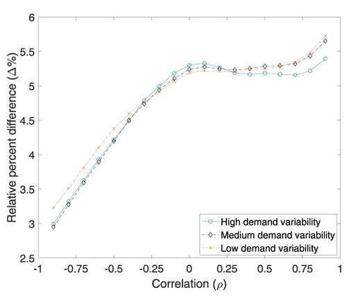
Figure 6 demonstrates how the variability of demand alongside the correlation between supply and demand affects the revenue improvement achieved through dynamic pricing policy. As the correlation value positively increases, the system experiences ‘Strong Supply-Strong Demand’ environment more often than not. Figure 6 indicates that dynamic pricing policy enhances the average profit as the correlation positively increases for the case in which the demand variability is not sufficiently high. When the system's state is ‘Strong Supply-Strong Demand’, high demand variability implies a higher demand, thereby increasing the expected profits that both constant and dynamic pricing strategies could achieve. Therefore, average profit enhancements with the dynamic pricing decline when the variability of demand is high.

We now turn our attention to the negative correlation, which corresponds to the cases where ‘Strong Supply-Poor Demand’ and ‘Poor Supply-Strong Demand’ environments are mostly present. As the correlation value among supply and demand environments negatively increases, experiencing low supply and demand variability positively affects the system's operations so that the system operator could harness both environments to enhance the sales of the final products. Observing low demand variability provides such an opportunity to the system to make a profit in both environments, although the profit-margin remains low in ‘Strong Supply-Poor Demand’ and ‘Poor Supply-Strong Demand’. Hence, pricing the final product dynamically based on changing conditions enables the system to generate a higher profit when the demand variability is low, and the correlation relationship among the supply and demand processes is considerably negative.

4.6.2. Effects of customer's price sensitivity and procurement price variability on the profit enhancement

Figure 7 demonstrates how both the degree of price-sensitivity of the market and procurement price variability affect the profit improvements that the system operator could obtain through dynamic pricing.

Figure 7. The price sensitivity and procurement price variability effects on the relative difference between dynamic and static pricing strategies.

For three different levels of price variability, this line graph depicts the profit improvement of using dynamic pricing relative to static pricing as the price sensitivity level varies between 0.5 and 1.

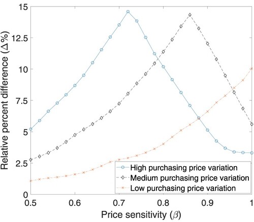
Figure 7 suggests that employing dynamic pricing generates higher profits in the presence of a price-sensitive market and a degree of procurement price variability, each of which affects the degree of profit enhancement that the dynamically pricing final products engender at various levels. Dynamic pricing policy increases the profit improvement for the set of values of price sensitivity parameter less than a particular threshold value, regardless of the degree of procurement price variability the system experiences. As the level of price sensitivity increases, the market becomes more price-sensitive, and the range of various price points the system operator can extend shrinks. Thus, the operator cannot exploit the benefit of setting the price levels of the final product based on the state variables, which decreases the profit improvement that dynamic pricing policy achieves.

The computational experiment that we conduct in this study indicates that the threshold value of the price sensitivity parameter at which the policy of dynamic pricing generates the highest profit improvement increases as the degree of the variability in procurement price decreases. When the procurement price variation is high, the system operator can find the raw material at a lower price, which leads the system to expand the profit margin by increasing the selling price of the product through dynamic pricing. Conversely, when the procurement price remains relatively stable, i.e. when the variability is low, the system operator cannot fully exploit the market, and, in turn, the profit improvement of dynamic pricing remains limited. For example, when procurement price variability is high (medium), dynamic pricing policy generates the highest additional profit improvement of approximately $15\mathrm{\%}$ $\left(14\mathrm{\%}\right)$ at $\text{β}\approx 0.7$ $(\text{β}\approx 0.85)$. Beyond the corresponding values of β, i.e. 0.7 and 0.85, the profit impact of employing dynamic pricing decreases gradually as the market gets more price-sensitive in both cases. A similar observation can be made for the case where procurement price variability is low.

4.6.3. Effects of production rate and holding cost on the profit enhancement

Figure 8 demonstrates how dynamic pricing brings additional profits as we change the production rate together with the unit holding cost of the product.

Figure 8. Effects of production rate and holding cost on the relative difference between dynamic and static pricing strategies.

For three different levels of holding cost, this line graph depicts the profit improvement of using dynamic pricing relative to static pricing as the production rate varies between 0.12 and 1.53.

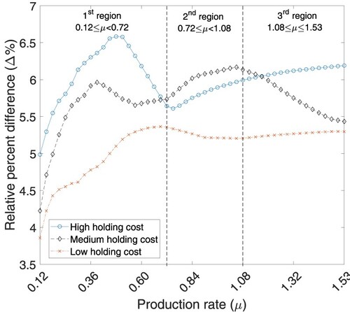
We note that in the analysis aimed at presenting effects of both the production rate and the holding cost on the system's profit, we cluster the range of values of production rate, i.e. μ, in Figure 8 into three distinct regions based on the relationship between supply and demand rates. The first region, which corresponds to the range of μ values less than 0.72, i.e. $\mu <0.72$, represents the case in which the production rate is less than the demand rate. The second region comprises μ values greater than or equal to 0.72 and less than 1.08, i.e. $0.72\le \mu <1.08$, which embraces two demand-supply structures: (i) in ‘Poor Demand’ environments, the system has an excessive production capacity, i.e. ${\mathrm{\Lambda }}_L<\mu$, and (ii) in ‘Strong Demand’ environments, the system has a limited production capacity, i.e. ${\mathrm{\Lambda }}_H>\mu$. Finally, the third region includes all possible μ values beyond 1.08, corresponding to the scenario in which the production rate comes to be greater than the demand rate; that is, the system has an excessive capacity.

When the production rate is less than the expected demand, which corresponds to μ values below 0.72, pricing the final products dynamically enhances the average profit up to $6.5\mathrm{\%}$ compared to that of the benchmark policy. When the units of the product that the system can produce are limited, the operator effectively utilises the final product inventory through dynamic pricing. For instance, when the final product inventory level is sufficiently high, the system operator can lower the selling price to stimulate demand. Conversely, as the number of units of the product in the second inventory decreases, the system operator might find it beneficial to increase the price level to a higher level both to increase the expected profit and to store some units of the product in inventory, serving as a buffer against randomly changing environment states. Moreover, Figure 8 shows that an increase in the unit holding cost of final products engenders the positive impact of dynamic pricing on the average profit; the flexibility of dynamically adjusting the price levels attenuates the negative effect of a higher holding cost on the system's profit.

As the production rate, μ varies between $0.72\le \mu <1.08$, the system, on average, experiences both limited and excess production capacities evenly. The resulting environment that envelops the system affects profit enhancements obtained through the dynamic pricing policy. Unit holding cost of the final products is decisive in the revenue improvement that dynamic pricing engenders. Figure 8 shows that the flexibility to adjust the final product's price level becomes effective when the final product's unit holding cost is sufficiently high. For example, when the unit holding cost is high, the system operator may lower the selling price to stimulate demand for the final product. On the other hand, when the unit holding cost is relatively low, she may prefer being selective, elevating the price point.

When the system operates with sufficient capacity, i.e. $\mu \ge 1.08$, dynamic pricing policy yields a higher profit of at least $5\mathrm{\%}$ greater than that of the benchmark policy, regardless of the unit holding cost of the final product. Figure 8 demonstrates that as the unit holding cost decreases, the marginal value of the product diminishes, which, in turn, decreases the revenue impact of the dynamic pricing policy. Besides, in this region, the profit impact of dynamic pricing exceedingly depends on the number of finished products the manufacturer stores on average. For instance, when the unit holding cost is medium, the average number of finished goods kept in inventory is higher than the cases where the unit holding cost is either low or high, thereby lowering the marginal value of one unit of finished goods in inventory. Hence, the additional profit that could be brought in by dynamic pricing declines. When the holding cost is either low or high, the average number of finished goods stored in inventory is less than the amount that the manufacturer would keep if it pursues constant pricing strategy, so dynamic pricing policy generates relatively more profit, as presented in the third region of Figure 8.

4.7. Managerial insights

In this section, we summarise our key findings from our numerical experiments to provide managerial insights into firms having the flexibility to follow dynamic pricing strategies or planning to use a similar pricing strategy. This study is mainly motivated by agricultural firms, so the following discussions are established employing this point of view. Nevertheless, it is also worth noting that these findings can be adapted to other business contexts as long as they have similar operational characteristics to those we consider in this work.

For a firm that operates in the agricultural industry, the efficacy of dynamic pricing is mainly dependent on the relationship between the supply amount of harvested materials and the demand for the end product, along with demand variability. Dynamic pricing could not significantly improve profit when the demand variability is high. In the case of moderate demand variability, dynamic pricing could be used as a profit-enhancing mechanism when both the amount of harvested materials and the demand are either high or low. In the case of low demand variability, pursuing the policy of dynamic pricing could enhance the firm's expected profit either when there is a dearth of harvested raw materials or when the firm has excessive supply, as we compare it with the demand process.

Moreover, the relationship between the production rate of the firm and the expected demand rate affects the extent to which dynamic pricing generates additional profit. In the case of a lesser production rate than the expected demand rate, which corresponds to the scenario where the firm may keep a considerable amount of harvested raw materials in inventory to meet demand, the profit impact of dynamic pricing is of the utmost in performance. If the firm's production rate is more or less the same or greater than the expected demand rate, then, on average, the firm either may not have to keep the harvested raw materials as opposed to the case where it would have to store them in the low production rate case in inventory or may lessen the amount of harvested raw materials held in inventory. Therefore, the flexibility of adjusting price levels with respect to the inventory levels dynamic pricing brings would decrease.

The variation in procurement price, too, impacts the efficacy of dynamic pricing in terms of the expected profit achieved by the firm. When the variation in the price point at which the firm procures the raw materials that are eventually turned into a finished product is relatively high, dynamic pricing could generate additional profit: the firm is capable of adjusting its sale price levels in accordance with the fluctuation in procurement price through dynamic pricing.

5. Conclusion and future works

We study an integrated problem of procurement, manufacturing, and pricing policies for a continuous-review make-to-stock system operating in a randomly fluctuating environment with exponentially distributed processing times. The random environment evolves according to a continuous-time discrete-state space Markov process, which directly affects the system's demand and supply processes, i.e, procurement prices, raw material flow rates, and price-dependent demand arrival rates. We model this system as an infinite-horizon Markovian decision process with the objective of maximising the long-run average profit. Besides, to numerically determining the optimal procurement, manufacturing, and pricing control strategies of the system, we develop a linear programming formulation of the problem.

Following the event-based dynamic programming framework given in Koole (1998), we first present several analytical results on the optimal control strategies. We establish that the optimal procurement and manufacturing strategies are of state-dependent threshold type policies and show that their threshold levels are monotone with respect to the final product and raw material inventory levels. On the other hand, the optimal dynamic pricing policy exhibits a monotonically decreasing structure, i.e. the optimal sale prices decrease as both final product and raw material inventory levels increase. This result comes from the fact that lowering sale prices does not only allow the manufacturer to sell more products but also to reduce her holding cost regarding on-hand inventory. Furthermore, we prove the existence of a state-dependent solution for the optimal price when the demand arrival rate has a linear form. In the analysis, we assume that the holding cost does not change with the environment. This assumption basically allows us to focus on the relation between supply and demand processes directly, which is our primary goal in this work. On the other hand, we should note that the structural results will still be valid when the assumptions of the model are generalised to include environment-dependent inventory holding cost functions as long as each holding cost function is convex and non-decreasing in the first and second inventory levels for all environment states.

We carry out a numerical analysis on the potential benefits of using a dynamic pricing strategy compared to a static pricing strategy when the demand function is linear. With this effort, it is demonstrated that the profit enhancement over static pricing by dynamic pricing is worth considering and that it can reach about 15% under certain conditions. This analysis can be valuable for the firms that intend to employ dynamic pricing instead of static pricing because it allows them to observe to what extent and under what circumstances dynamic pricing strategies can lead to a significant improvement in their profits. But, they should also consider this analysis a rather optimistic comparison since we do not take into account certain intangible negative impacts of dynamic pricing such as burden costs of making frequent price changes, lack of experience in its implementation, and possible adverse customer reactions.

Furthermore, our study, through an extensive numerical study, helps practitioners pave the way for the efficient implementation of dynamic pricing strategies in the presence of uncertainty on the supply and demand sides. Our numerical study suggests that dynamic pricing could enhance the firm's expected profit when there is a positive correlation between supply and demand processes and the variability of the demand process is not sufficiently high. When the demand variability is sufficiently high, the profit impact of dynamic pricing remains limited. In the case of a negative correlation between supply and demand processes, dynamic pricing can be used as a tool to increase the expected long-run profit, mainly when the demand variability is relatively low. Secondly, our numerical study demonstrates that the profit impact of dynamically pricing the finished product becomes significant (insignificant) when the procurement price variability is high (low). Lastly, the profit impact of dynamic pricing is dependent on the production rate that the facility owns. When the production rate of the facility is less than the expected demand rate, the value of each unit of the finished product inventory increases, and the firm can enhance the expected profit by dynamically setting the price level of the finished product, depending on the finished product inventory. In the case of a sufficiently higher production rate than the expected demand rate, the firm does not benefit from dynamic pricing in the pursuit of the expected profit enhancement. When the firm observes both limited and excess production capacities uniformly, the unit inventory cost of the finished product becomes decisive: the firm improves the expected profit with dynamic pricing if the unit holding cost is low. Otherwise, the profit improvement dynamic pricing brings about remains limited if the unit holding cost is high.

Our work can be extended in several ways. In this work, we essentially give an analytical point of view on integrated procurement, manufacturing, and pricing decisions for a make-to-stock system having a single product and a reliable production facility. Extending this work to a setting with multiple products and an unreliable facility would enable us to investigate the impacts of maintenance and capacity-allocation decisions on the system. In the mathematical model that we propose to address the given problem setting, we use the assumption of exponentially distributed processing, demand inter-arrival, and raw material inter-arrival times. This assumption allows us to use the existing Markov theory, thereby facilitating the system analysis and the derivation of analytical results. Although this assumption is sufficient to represent many examples in practice, demand inter-arrival, raw material inter-arrival, and processing times can follow a distribution different from exponential distribution in some particular cases. Therefore, covering the scenarios that do not require exponentially distributed processing, demand inter-arrival, and raw material inter-arrival times will be a valuable topic for future research. But, it should also be noted that such an extension will make the analysis cumbersome and not make it easier to derive analytical results. Another interesting line of extension is to consider the existence of strategic customers and to model their choice behaviours explicitly. Incorporating this type of customer modeling into our work would be challenging because of its computational and analytical complexity. However, it would definitely allow us to generalise our findings further. Lastly, in the current model, the system operator is assumed to be capable of observing all environmental changes and their transition rates fully and perfectly. Extending this assumption to cover both uncertain environment transition rates and unobservable environments would be an interesting and valuable path for future research.

Acknowledgments

We would like to acknowledge Dr. Rommert Dekker from Erasmus University Rotterdam and Dr. Barış Tan from Koç University for their valuable remarks that helped us to improve this work. We also would like to thank the associate editor and the anonymous reviewers for their valuable comments and suggestions.

Disclosure statement

No potential conflict of interest was reported by the author(s).

Data availability statement

Data sharing is not applicable to this article as no new data were created or analysed in this study.

Additional information

Notes on contributors

Oktay Karabağ

Oktay Karabağ is an assistant professor at Yaşar University and a visiting research fellow at Erasmus University Rotterdam. Before joining Yaşar University, between 2019–2021, he worked as an assistant professor in the School of Economics at Erasmus University Rotterdam. Between 2018–2019, he also worked as a post-doctoral researcher on an industry-oriented research project at Eindhoven University of Technology. He completed his Ph.D. studies at the Department of Industrial Engineering and Operations Management at Koç University. He received a B.S. degree in Statistics from Ege University and a master's degree in Intelligent Production Systems Engineering from İzmir University of Economics. His current research interests include stochastic modeling, design and control of manufacturing systems, maintenance optimisation, and cooperation in supply chain management.

Burak Gökgür

Burak Gökgür is an Assistant Professor of Operations Management at Sabancı University, Istanbul, Turkey. His research interests are supply chain management, retail operations, revenue management, and the interface of operations management and marketing. He holds a B.S. degree in Industrial Systems Engineering and an M.Sc. in Intelligent Production Systems from the İzmir University of Economics (İzmir, Turkey). He received his Ph.D. in Operations Management from Koç University (İstanbul, Turkey).

Appendices

Appendix 1.

Theorem proofs

We utilise the event-based dynamic programming techniques of Koole (1998) in order to characterise the optimal control policies for procurement, manufacturing, and pricing decisions. We first transform the maximisation problem we consider in the main text into an equivalent minimisation problem because this modified version of the problem facilitates our proofs by making it possible to use the findings derived in Koole (2004) and Karabağ and Tan (2019) directly. The optimality equation regarding the modified version of the problem is: (A1) $\begin{array}{rl}{\varphi }^{\mathrm{\prime }}(e,\underset{\_}{i})+q^{\ast }& =V_g^{\mathrm{\prime }}{\varphi }^{\mathrm{\prime }}(e,\underset{\_}{i})+V_p^{\mathrm{\prime }}{\varphi }^{\mathrm{\prime }}(e,\underset{\_}{i})+V_z^{\mathrm{\prime }}{\varphi }^{\mathrm{\prime }}(e,\underset{\_}{i})\\ & +V_f\varphi (e,\underset{\_}{i})-(c^{h_1}{i}_1+c^{h_2}{i}_2),\end{array}$(A1) where ${\varphi }^{\mathrm{\prime }}(e,\underset{\_}{i})=-\varphi (e,\underset{\_}{i})$. On the other hand, for any real function $\theta (e,\underset{\_}{i})$, the operators appeared in Equation (A1(A1) $\begin{array}{rl}{\varphi }^{\mathrm{\prime }}(e,\underset{\_}{i})+q^{\ast }& =V_g^{\mathrm{\prime }}{\varphi }^{\mathrm{\prime }}(e,\underset{\_}{i})+V_p^{\mathrm{\prime }}{\varphi }^{\mathrm{\prime }}(e,\underset{\_}{i})+V_z^{\mathrm{\prime }}{\varphi }^{\mathrm{\prime }}(e,\underset{\_}{i})\\ & +V_f\varphi (e,\underset{\_}{i})-(c^{h_1}{i}_1+c^{h_2}{i}_2),\end{array}$(A1) ), $V_g^{\mathrm{\prime }}\theta (e,\underset{\_}{i})$, $V_p^{\mathrm{\prime }}\theta (e,\underset{\_}{i})$, and $V_z^{\mathrm{\prime }}\theta (e,\underset{\_}{i})$ are defined as: (A2) $\begin{array}{rl}{V}_g^{\mathrm{\prime }}\theta (e,\underset{\_}{i})& =min\{{\delta }_e\theta (e,\underset{\_}{i}+u_1)+{\delta }_e{c}_e^g,{\delta }_e\theta (e,\underset{\_}{i})\},\end{array}$(A2) (A3) $\begin{array}{rl}{V}_p^{\mathrm{\prime }}\theta (e,\underset{\_}{i})& =\{\begin{array}{ll}\begin{array}{l}min\left\{\mu \right(\theta (e,\underset{\_}{i}-u_1+u_2)\\ +c^p),\mu \theta (e,\underset{\_}{i}\left)\right\},\end{array}& i_1>0,\\ \mu \theta (e,\underset{\_}{i}),& i_1=0,\end{array}\end{array}$(A3) (A4) $\begin{array}{rl}{V}_z^{\mathrm{\prime }}\theta (e,\underset{\_}{i})& =\{\begin{array}{ll}\begin{array}{l}\underset{s\in {\mathcal{D}}^{\mathrm{\prime }}}{min}\{-{\omega }_e(s)+{\lambda }_e(s\left)\theta \right(e,\underset{\_}{i}-u_2)\\ +({\mathrm{\Lambda }}_e-{\lambda }_e(s\left)\right)\theta (e,\underset{\_}{i})\}\end{array}& i_2>0,\\ {\mathrm{\Lambda }}_e\theta (e,\underset{\_}{i}),& i_2=0.\end{array}\end{array}$(A4) Note that Equations (A1(A1) $\begin{array}{rl}{\varphi }^{\mathrm{\prime }}(e,\underset{\_}{i})+q^{\ast }& =V_g^{\mathrm{\prime }}{\varphi }^{\mathrm{\prime }}(e,\underset{\_}{i})+V_p^{\mathrm{\prime }}{\varphi }^{\mathrm{\prime }}(e,\underset{\_}{i})+V_z^{\mathrm{\prime }}{\varphi }^{\mathrm{\prime }}(e,\underset{\_}{i})\\ & +V_f\varphi (e,\underset{\_}{i})-(c^{h_1}{i}_1+c^{h_2}{i}_2),\end{array}$(A1) )–(A4(A4) $\begin{array}{rl}{V}_z^{\mathrm{\prime }}\theta (e,\underset{\_}{i})& =\{\begin{array}{ll}\begin{array}{l}\underset{s\in {\mathcal{D}}^{\mathrm{\prime }}}{min}\{-{\omega }_e(s)+{\lambda }_e(s\left)\theta \right(e,\underset{\_}{i}-u_2)\\ +({\mathrm{\Lambda }}_e-{\lambda }_e(s\left)\right)\theta (e,\underset{\_}{i})\}\end{array}& i_2>0,\\ {\mathrm{\Lambda }}_e\theta (e,\underset{\_}{i}),& i_2=0.\end{array}\end{array}$(A4) ) are equivalent to the maximisation versions of Equations (4(4) $\begin{array}{rl}\varphi (e,\underset{\_}{i})+q^{\ast }& =V_g\varphi (e,\underset{\_}{i})+V_p\varphi (e,\underset{\_}{i})+V_z\varphi (e,\underset{\_}{i})\\ & +V_f\varphi (e,\underset{\_}{i})-(c^{h_1}{i}_1+c^{h_2}{i}_2),\end{array}$(4) )–(7(7) $\begin{array}{rl}{V}_z\theta (e,\underset{\_}{i})& =\{\begin{array}{l}\underset{s\in {\mathcal{D}}^{\mathrm{\prime }}}{max}\left\{{\omega }_e\right(s)\\ +{\lambda }_e\left(s\right)\theta (e,\underset{\_}{i}-u_2)\\ +({\mathrm{\Lambda }}_e-{\lambda }_e(s\left)\right)\theta (e,\underset{\_}{i})\}& i_2>0,\\ {\mathrm{\Lambda }}_e\theta (e,\underset{\_}{i}),& i_2=0,\end{array}\end{array}$(7) ), respectively.

We consider that the optimal value function belonging to the modified version of the problem satisfies the property specified in the following paragraphs for all states. Let Ω be a set of real-valued functions on ${\mathbb{Z}}^3$ such that if ${\varphi }^{\mathrm{\prime }}(e,\underset{\_}{i})\in \mathrm{\Omega }$, then it satisfies (A5) $\begin{array}{r}{\varphi }^{\mathrm{\prime }}(e,\underset{\_}{i})+{\varphi }^{\mathrm{\prime }}(e,\underset{\_}{i}+f+f^{\mathrm{\prime }})\le {\varphi }^{\mathrm{\prime }}(e,\underset{\_}{i}+f)+{\varphi }^{\mathrm{\prime }}(e,\underset{\_}{i}+f^{\mathrm{\prime }}),\end{array}$(A5) for all $\underset{\_}{i}\in {\mathbb{Z}}^2$ and $f,f^{\mathrm{\prime }}\in \mathcal{F}=\{u_1,u_2-u_1,-u_2\}$ with $f\ne f^{\mathrm{\prime }}$. Essentially, the expression presented in Equation (A5(A5) $\begin{array}{r}{\varphi }^{\mathrm{\prime }}(e,\underset{\_}{i})+{\varphi }^{\mathrm{\prime }}(e,\underset{\_}{i}+f+f^{\mathrm{\prime }})\le {\varphi }^{\mathrm{\prime }}(e,\underset{\_}{i}+f)+{\varphi }^{\mathrm{\prime }}(e,\underset{\_}{i}+f^{\mathrm{\prime }}),\end{array}$(A5) ) corresponds to the inequality that needs to be satisfied for having multi-modularity with respect to both $i_1$ and $i_2$. It is known that if ${\varphi }^{\mathrm{\prime }}(e,\underset{\_}{i})$ meets the inequality given for having multi-modularity, it also meets the inequalities that need to be satisfied for having component-wise convexity. For a detailed proof of this result, we refer to the works of Koole (2004) and Karabağ and Tan (2019). Mathematically, the condition of being component-wise convex is given in Lemma A.1.

Lemma A.1

If ${\varphi }^{\mathrm{\prime }}(e,\underset{\_}{i})\in \mathrm{\Omega }$, then it also satisfies the inequality below: (A6) $\begin{array}{r}2{\varphi }^{\mathrm{\prime }}(e,\underset{\_}{i}+u_k)\le {\varphi }^{\mathrm{\prime }}(e,\underset{\_}{i})+{\varphi }^{\mathrm{\prime }}(e,\underset{\_}{i}+2u_k),\mathrm{\forall }\underset{\_}{i}\in {\mathbb{Z}}^2,\end{array}$(A6) where $k\in \{1,2\}$.

On the other hand, the property of multi-modularity is known to imply the property of joint convexity, as well (Altman, Gaujal, and Hordijk 2000; Karabağ and Tan 2019). That is, if ${\varphi }^{\mathrm{\prime }}(e,\underset{\_}{i})$ meets the inequality given for having multi-modularity, it evidently meets the inequalities for having joint convexity. So, we get:

Lemma A.2

If ${\varphi }^{\mathrm{\prime }}(e,\underset{\_}{i})\in \mathrm{\Omega }$, then it is jointly convex in both $i_1$ and $i_2$.

Lastly, Lemma A.3 reveals that for all environment states, the operator V preserves the properties of joint convexity, component-wise convexity, and multi-modularity.

Lemma A.3

If ${\varphi }^{\mathrm{\prime }}(e,\underset{\_}{i})\in \mathrm{\Omega }$, then $V{\varphi }^{\mathrm{\prime }}(e,\underset{\_}{i})$, where $V{\varphi }^{\mathrm{\prime }}(e,\underset{\_}{i})=V_g^{\mathrm{\prime }}{\varphi }^{\mathrm{\prime }}(e,\underset{\_}{i})+V_m^{\mathrm{\prime }}{\varphi }^{\mathrm{\prime }}(e,\underset{\_}{i})+V_z^{\mathrm{\prime }}{\varphi }^{\mathrm{\prime }}(e,\underset{\_}{i})+V_f\varphi (e,\underset{\_}{i})+(c^{h_1}{i}_1+c^{h_2}{i}_2)$, preserves the properties of joint convexity, component-wise convexity, and multi-modularity.

Proof

Proof of Lemma A.3

By assumption, the holding cost has a linear structure, therefore, it directly preserves all the given properties. In the work of Koole (2004), the operators $V_g^{\mathrm{\prime }}\theta (e,\underset{\_}{i})$, $V_p^{\mathrm{\prime }}\theta (e,\underset{\_}{i})$, and $V_z^{\mathrm{\prime }}\theta (e,\underset{\_}{i})$ are already shown to preserve the multi-modularity property when any real-valued function $\theta (e,\underset{\_}{i})$ is multi-modular. It is also evident that they will retain the properties of joint and component-wise convexity because of Lemmas A.1 and A.2. On the other hand, $V_f\theta (e,\underset{\_}{i})$ is structured as a linear combination of $\theta (e,\underset{\_}{i})$, implying that the relevant operator preserves the properties of joint convexity, component-wise convexity, and multi-modularity. Consequently, as each operator being used to establish V preserves joint convexity, component-wise convexity, and multi-modularity, V will also retain these properties.

Considering the value iteration principle together with Lemma A.3, we can conclude that the optimal value function ${\varphi }^{\mathrm{\prime }\ast }(e,\underset{\_}{i})$ meets the inequalities that need to be held for having the properties of joint and component-wise convexity. This conclusion directly implies the existence of a unique threshold level for procurement and manufacturing decisions and of a unique solution for pricing decisions. In what follows, we present the proofs of our analytical findings related to these decisions in detail.

Proof

Proof of Theorem 3.1

Let ${\varphi }^{\mathrm{\prime }\ast }(e,\underset{\_}{i})\in \mathrm{\Omega }$. It is known that any real-valued function ${\varphi }^{\mathrm{\prime }\ast }(e,\underset{\_}{i})$ satisfying the inequalities for multi-modularity will also meet the inequalities for component-wise convexity (Karabağ and Tan 2019). Accordingly, we get: (A7) $\begin{array}{r}{\varphi }^{\mathrm{\prime }\ast }(e,\underset{\_}{i}+u_1)-{\varphi }^{\mathrm{\prime }\ast }(e,\underset{\_}{i})\ge {\varphi }^{\mathrm{\prime }\ast }(e,\underset{\_}{i})-{\varphi }^{\mathrm{\prime }\ast }(e,\underset{\_}{i}-u_1).\end{array}$(A7) Let's suppose that for $(e,\underset{\_}{i})$, the optimum decision is to procure a unit of raw material. In such a case, Equation (A2(A2) $\begin{array}{rl}{V}_g^{\mathrm{\prime }}\theta (e,\underset{\_}{i})& =min\{{\delta }_e\theta (e,\underset{\_}{i}+u_1)+{\delta }_e{c}_e^g,{\delta }_e\theta (e,\underset{\_}{i})\},\end{array}$(A2) ) gives the following expression: (A8) $\begin{array}{rl}& {\varphi }^{\mathrm{\prime }\ast }(e,\underset{\_}{i}+u_1)+c_e^g<{\varphi }^{\mathrm{\prime }\ast }(e,\underset{\_}{i})\\ & ⟺{\varphi }^{\mathrm{\prime }\ast }(e,\underset{\_}{i}+u_1)-{\varphi }^{\mathrm{\prime }\ast }(e,\underset{\_}{i})<-c_e^g.\end{array}$(A8) Then, considering the convexity in the direction of $u_1$, we get: (A9) $\begin{array}{r}-c_e^g>{\varphi }^{\mathrm{\prime }\ast }(e,\underset{\_}{i}+u_1)-{\varphi }^{\mathrm{\prime }\ast }(e,\underset{\_}{i})\ge {\varphi }^{\mathrm{\prime }\ast }(e,\underset{\_}{i})-{\varphi }^{\mathrm{\prime }\ast }(e,\underset{\_}{i}-u_1).\end{array}$(A9) Equation (A9(A9) $\begin{array}{r}-c_e^g>{\varphi }^{\mathrm{\prime }\ast }(e,\underset{\_}{i}+u_1)-{\varphi }^{\mathrm{\prime }\ast }(e,\underset{\_}{i})\ge {\varphi }^{\mathrm{\prime }\ast }(e,\underset{\_}{i})-{\varphi }^{\mathrm{\prime }\ast }(e,\underset{\_}{i}-u_1).\end{array}$(A9) ) evidently means that it is also optimal to procure in $(e,\underset{\_}{i}-u_1)$. On the basis of this result, we can say that the optimum decision is to procure in all states $(e,\widetilde{\underset{\_}{i}})$ where $\widetilde{\underset{\_}{i}}=({\tilde{i}}_1,i_2)$ and ${\tilde{i}}_1<i_1$ if it is optimal to procure in $(e,\underset{\_}{i})$ where $\underset{\_}{i}=(i_1,i_2)$. Similarly, we can also prove that the optimum decision is not to procure in all states $(e,\widehat{\underset{\_}{i}})$ where $\underset{\_}{\hat{i}}=({\hat{i}}_1,i_2)$ and ${\hat{i}}_1\ge i_1$ if it is optimal not to procure in $(e,\underset{\_}{i})$ where $\underset{\_}{i}=(i_1,i_2)$. These two statements reveal that there exists a unique optimum threshold level for the procurement decision.

So, for any given state $(e,\underset{\_}{i})$ where $(i_1,i_2)$, the corresponding threshold level can mathematically be written as follows: (A10) $\begin{array}{r}{X}_g^{\ast }(e,i_2)=\arg \underset{i_1}{min}\left\{(e,i_1,i_2)\right|d_g^{\ast }(e,i_1,i_2)=0\}.\end{array}$(A10) The optimisation problem given in Equation (A10(A10) $\begin{array}{r}{X}_g^{\ast }(e,i_2)=\arg \underset{i_1}{min}\left\{(e,i_1,i_2)\right|d_g^{\ast }(e,i_1,i_2)=0\}.\end{array}$(A10) ) provides us with a unique threshold level $X_g^{\ast }(e,i_2)$, which allows for characterising the optimal procurement policy analytically for any given state $(e,\underset{\_}{i})$ where $(i_1,i_2)$. Specifically, the optimum decision is to procure if $X_g^{\ast }(e,i_2)>i_1$ and not to procure otherwise.

Proof

Proof of Theorem 3.2

Let ${\varphi }^{\mathrm{\prime }\ast }(e,\underset{\_}{i})\in \mathrm{\Omega }$. It is known that any real-valued function ${\varphi }^{\mathrm{\prime }\ast }(e,\underset{\_}{i})$ satisfying the inequalities for multi-modularity will also meet the inequalities for joint-convexity (Karabağ and Tan 2019). Accordingly, we get: (A11) $\begin{array}{rl}& {\varphi }^{\mathrm{\prime }\ast }(e,\underset{\_}{i}-u_1+u_2)-{\varphi }^{\mathrm{\prime }\ast }(e,\underset{\_}{i})\\ & \ge {\varphi }^{\mathrm{\prime }\ast }(e,\underset{\_}{i})-{\varphi }^{\mathrm{\prime }\ast }(e,\underset{\_}{i}+u_1-u_2).\end{array}$(A11) Let's suppose that for $(e,\underset{\_}{i})$, the optimum decision is to manufacture a unit of final product. In such a case, Equation (A3(A3) $\begin{array}{rl}{V}_p^{\mathrm{\prime }}\theta (e,\underset{\_}{i})& =\{\begin{array}{ll}\begin{array}{l}min\left\{\mu \right(\theta (e,\underset{\_}{i}-u_1+u_2)\\ +c^p),\mu \theta (e,\underset{\_}{i}\left)\right\},\end{array}& i_1>0,\\ \mu \theta (e,\underset{\_}{i}),& i_1=0,\end{array}\end{array}$(A3) ) yields the following expression: (A12) $\begin{array}{rl}& {\varphi }^{\mathrm{\prime }}(e,\underset{\_}{i}-u_1+u_2)+c^p<{\varphi }^{\mathrm{\prime }}(e,\underset{\_}{i})\\ & ⟺-c^p>{\varphi }^{\mathrm{\prime }}(e,\underset{\_}{i}-u_1+u_2)-{\varphi }^{\mathrm{\prime }}(e,\underset{\_}{i}).\end{array}$(A12) Then, considering the convexity in the direction of $(u_2-u_1)$, we get: (A13) $\begin{array}{rl}& -c^p>{\varphi }^{\mathrm{\prime }\ast }(e,\underset{\_}{i}-u_1+u_2)-{\varphi }^{\mathrm{\prime }\ast }(e,\underset{\_}{i})\\ & \ge {\varphi }^{\mathrm{\prime }\ast }(e,\underset{\_}{i})-{\varphi }^{\mathrm{\prime }\ast }(e,\underset{\_}{i}+u_1-u_2).\end{array}$(A13) Equation (A13(A13) $\begin{array}{rl}& -c^p>{\varphi }^{\mathrm{\prime }\ast }(e,\underset{\_}{i}-u_1+u_2)-{\varphi }^{\mathrm{\prime }\ast }(e,\underset{\_}{i})\\ & \ge {\varphi }^{\mathrm{\prime }\ast }(e,\underset{\_}{i})-{\varphi }^{\mathrm{\prime }\ast }(e,\underset{\_}{i}+u_1-u_2).\end{array}$(A13) ) evidently implies that it is also optimal to produce in $(e,\underset{\_}{i}+u_1-u_2)$. On the basis of this implication, we can say that the optimum decision is to manufacture in all states $(e,{\hat{i}}_1,{\hat{i}}_2)$ satisfying ${\hat{i}}_1+{\hat{i}}_2=k$ where ${\hat{i}}_1>i_1$ and ${\hat{i}}_2<k-{\hat{i}}_1$ if it is optimal to manufacture in $(e,i_1,i_2)$ where $i_1+i_2=k$. Similarly, we can also prove that the optimum decision is not to manufacture in all states $(e,{\tilde{i}}_1,{\tilde{i}}_2)$ satisfying ${\tilde{i}}_1+{\tilde{i}}_2=k$ where ${\tilde{i}}_1\le i_1$ and ${\tilde{x}}_2\ge k-{\tilde{x}}_1$ if it is optimal not to manufacture in $(e,i_1,i_2)$ where $i_1+i_2=k$. These two statements reveal that there exists a unique optimum threshold level for the manufacturing decision.

So, for any given state $(e,i_1,i_2)$ where $i_1+i_2=k$, the corresponding threshold level can mathematically be written as follows: (A14) $\begin{array}{r}{X}_p^{\ast }(e,i_2)=\arg \underset{i_1}{max}\left\{(e,i_1,k-i_1)\right|d_p^{\ast }(e,i_1,k-i_1)=0\}.\end{array}$(A14) The optimisation problem given in Equation (A14(A14) $\begin{array}{r}{X}_p^{\ast }(e,i_2)=\arg \underset{i_1}{max}\left\{(e,i_1,k-i_1)\right|d_p^{\ast }(e,i_1,k-i_1)=0\}.\end{array}$(A14) ) provides us with a unique threshold level $X_p^{\ast }(e,i_2)$, which allows for characterising the optimal manufacturing policy analytically for any given state $(e,i_1,i_2)$ where $i_1+i_2=k$. More specifically, the optimum decision is to manufacture if $i_1>X_p^{\ast }(e,i_2)$ and not to manufacture otherwise.

Proof

Proof of Theorem 3.3

The results we obtain in the proof of the first theorem evidently reveal that the threshold level for the procurement decision is non-ascending in $i_1$.

Let ${\varphi }^{\mathrm{\prime }\ast }(e,\underset{\_}{i})\in \mathrm{\Omega }$. It is known that any real-valued function ${\varphi }^{\mathrm{\prime }\ast }(e,\underset{\_}{i})$ satisfying the inequalities for multi-modularity will also meet the inequalities for super-modularity (Koole 1998,2004). Accordingly, we get: (A15) $\begin{array}{rl}& {\varphi }^{\mathrm{\prime }\ast }(e,\underset{\_}{i}+u_1+u_2)-{\varphi }^{\mathrm{\prime }\ast }(e,\underset{\_}{i}+u_2)\\ & \ge {\varphi }^{\mathrm{\prime }\ast }(e,\underset{\_}{i}+u_1)-{\varphi }^{\mathrm{\prime }\ast }(e,\underset{\_}{i}).\end{array}$(A15) Let's suppose that for $(e,\underset{\_}{i})$, the optimum decision is not to procure a unit of raw material. In such a case, Equation (A2(A2) $\begin{array}{rl}{V}_g^{\mathrm{\prime }}\theta (e,\underset{\_}{i})& =min\{{\delta }_e\theta (e,\underset{\_}{i}+u_1)+{\delta }_e{c}_e^g,{\delta }_e\theta (e,\underset{\_}{i})\},\end{array}$(A2) ) gives the following expression: (A16) $\begin{array}{r}{\varphi }^{\mathrm{\prime }\ast }(e,\underset{\_}{i}+u_1)-{\varphi }^{\mathrm{\prime }\ast }(e,\underset{\_}{i})>-c_e^g.\end{array}$(A16) Using Equations (A15(A15) $\begin{array}{rl}& {\varphi }^{\mathrm{\prime }\ast }(e,\underset{\_}{i}+u_1+u_2)-{\varphi }^{\mathrm{\prime }\ast }(e,\underset{\_}{i}+u_2)\\ & \ge {\varphi }^{\mathrm{\prime }\ast }(e,\underset{\_}{i}+u_1)-{\varphi }^{\mathrm{\prime }\ast }(e,\underset{\_}{i}).\end{array}$(A15) ) and (A16(A16) $\begin{array}{r}{\varphi }^{\mathrm{\prime }\ast }(e,\underset{\_}{i}+u_1)-{\varphi }^{\mathrm{\prime }\ast }(e,\underset{\_}{i})>-c_e^g.\end{array}$(A16) ), we can infer: (A17) $\begin{array}{rl}& {\varphi }^{\mathrm{\prime }\ast }(e,\underset{\_}{i}+u_1+u_2)-{\varphi }^{\mathrm{\prime }\ast }(e,\underset{\_}{i}+u_2)\\ & \ge {\varphi }^{\mathrm{\prime }\ast }(e,\underset{\_}{i}+u_1)-{\varphi }^{\mathrm{\prime }\ast }(e,\underset{\_}{i})>-c_e^g.\end{array}$(A17) The above inequality evidently means that it is optimal not to procure in $(e,\underset{\_}{i}+u_2)$, either. On the basis of this result, we can say that the optimum decision is not to procure in all states $(e,{\underset{\_}{i}}^{\mathrm{\prime }})$ where ${\underset{\_}{i}}^{\mathrm{\prime }}=(i_1,i_2^{\mathrm{\prime }})$ and $i_2^{\mathrm{\prime }}>i_2$ if it is optimal not to procure in $(e,\underset{\_}{i})$ where $\underset{\_}{i}=(i_1,i_2)$. Correspondingly, for any given two states $(e,i_1,i_2)$ and $(e,i_1,i_2^{\mathrm{\prime }})$ where $i_2^{\mathrm{\prime }}>i_2$, we have: (A18) $\begin{array}{r}{d}_g^{\ast }(e,i_1,i_2)\ge d_g^{\ast }(e,i_1,i_2^{\mathrm{\prime }}).\end{array}$(A18) Let $X_g^{\ast }(e,i_2)$ and $X_g^{\ast }(e,i_2^{\mathrm{\prime }})$ be the threshold levels for the procurement decisions in $(e,i_1,i_2)$ and $(e,i_1,i_2^{\mathrm{\prime }})$. Together with Equation (A18(A18) $\begin{array}{r}{d}_g^{\ast }(e,i_1,i_2)\ge d_g^{\ast }(e,i_1,i_2^{\mathrm{\prime }}).\end{array}$(A18) ), this implies that $X_g^{\ast }(e,i_2)\ge X_g^{\ast }(e,i_2^{\mathrm{\prime }})$. Correspondingly, we can conclude that $X_g^{\ast }(e,i_2)$ defining the procurement decision's threshold level in $(e,i_1,i_2)$ is non-ascending with respect to $i_2$.

Proof

Proof of Theorem 3.4

Let ${\varphi }^{\mathrm{\prime }\ast }(e,\underset{\_}{i})\in \mathrm{\Omega }$. It is known that any real-valued function ${\varphi }^{\mathrm{\prime }\ast }(e,\underset{\_}{i})$ satisfying the inequalities for multi-modularity will also meet the inequalities for super-convexity (Koole 1998, 2004). Accordingly, we get: (A19) $\begin{array}{rl}& {\varphi }^{\mathrm{\prime }\ast }(e,\underset{\_}{i}+u_2)-{\varphi }^{\mathrm{\prime }\ast }(e,\underset{\_}{i}+u_1)\\ & \le {\varphi }^{\mathrm{\prime }\ast }(e,\underset{\_}{i}-u_1+u_2)-{\varphi }^{\mathrm{\prime }\ast }(e,\underset{\_}{i}).\end{array}$(A19) Let's suppose that for $(e,\underset{\_}{i})$, the optimum decision is to manufacture a unit of final product. In such a case, Equation (A3(A3) $\begin{array}{rl}{V}_p^{\mathrm{\prime }}\theta (e,\underset{\_}{i})& =\{\begin{array}{ll}\begin{array}{l}min\left\{\mu \right(\theta (e,\underset{\_}{i}-u_1+u_2)\\ +c^p),\mu \theta (e,\underset{\_}{i}\left)\right\},\end{array}& i_1>0,\\ \mu \theta (e,\underset{\_}{i}),& i_1=0,\end{array}\end{array}$(A3) ) yields the following expression: (A20) $\begin{array}{r}{\varphi }^{\mathrm{\prime }}(e,\underset{\_}{i}-u_1+u_2)-{\varphi }^{\mathrm{\prime }}(e,\underset{\_}{i})<-c^p.\end{array}$(A20) Using Equations (A19(A19) $\begin{array}{rl}& {\varphi }^{\mathrm{\prime }\ast }(e,\underset{\_}{i}+u_2)-{\varphi }^{\mathrm{\prime }\ast }(e,\underset{\_}{i}+u_1)\\ & \le {\varphi }^{\mathrm{\prime }\ast }(e,\underset{\_}{i}-u_1+u_2)-{\varphi }^{\mathrm{\prime }\ast }(e,\underset{\_}{i}).\end{array}$(A19) ) and (A20(A20) $\begin{array}{r}{\varphi }^{\mathrm{\prime }}(e,\underset{\_}{i}-u_1+u_2)-{\varphi }^{\mathrm{\prime }}(e,\underset{\_}{i})<-c^p.\end{array}$(A20) ), we can infer: (A21) $\begin{array}{rl}& {\varphi }^{\mathrm{\prime }\ast }(e,\underset{\_}{i}+u_2)-{\varphi }^{\mathrm{\prime }\ast }(e,\underset{\_}{i}+u_1)\\ & \le {\varphi }^{\mathrm{\prime }\ast }(e,\underset{\_}{i}-u_1+u_2)-{\varphi }^{\mathrm{\prime }\ast }(e,\underset{\_}{i})<-c^p.\end{array}$(A21) The above inequality evidently implies that it is optimal to manufacture in $(e,\underset{\_}{i}+u_1)$, either. On the basis of this implication, we can say that the optimum decision is to manufacture in all states $(e,\widehat{\underset{\_}{i}})$ where $\widehat{\underset{\_}{i}}=({\hat{i}}_1,i_2)$ and ${\hat{i}}_1>i_1$ if it is optimal to manufacture in $(e,\underset{\_}{i})$ where $\underset{\_}{i}=(i_1,i_2)$. Correspondingly, for any given two states $(e,i_1,i_2)$ and $(e,{\hat{i}}_1,i_2)$ where ${\hat{i}}_1>i_1$, we have: (A22) $\begin{array}{r}{d}_p^{\ast }(e,i_1,i_2)\le d_p^{\ast }(e,{\hat{i}}_1,i_2).\end{array}$(A22) Let $X_p^{\ast }(e,i_2)$ and $X_p^{\ast }(e,i_2)$ be the threshold levels for the manufacturing decisions in $(e,i_1,i_2)$ and $(e,{\hat{i}}_1,i_2)$. Together with Equation (A22(A22) $\begin{array}{r}{d}_p^{\ast }(e,i_1,i_2)\le d_p^{\ast }(e,{\hat{i}}_1,i_2).\end{array}$(A22) ), this implies that $X_p^{\ast }(e,i_2)\le X_p^{\ast }(e,i_2)$. Correspondingly, we can conclude that $X_p^{\ast }(e,i_2)$ defining the manufacturing decision's threshold level in $(e,i_1,i_2)$ is non-descending with respect to $i_1$.

Analogously, it can be proved that the relevant threshold level is non-ascending with respect to $i_2$, either. For the sake of clarity, we skip the corresponding proof.

Proof

Proof of Theorem 3.5

Let $s^{\ast }$ be the optimum sale price for $(e,i_1,i_2)$. For any given $i_1>0$, $s^{\ast }$ is the unique minimiser of the following function: (A23) $\begin{array}{rl}& \sigma (s,(e,i_1,i_2))\\ & =-{\omega }_e\left(s\right)-{\lambda }_e\left(s\right)[{\varphi }^{\mathrm{\prime }}(e,i_1,i_2)-{\varphi }^{\mathrm{\prime }}(e,i_1,i_2-1)],\end{array}$(A23) (A24) $\begin{array}{rl}& =-{\omega }_e\left(s\right)-{\lambda }_e\left(s\right)\mathrm{\Delta }{\varphi }_d^{\mathrm{\prime }}(e,i_1,i_2-1).\end{array}$(A24) All terms of the equation given above are convex in s, resulting in that the function itself is also convex in s. So, for the given equation, there definitely exists a unique minimiser $s^{\ast }$ on $\mathcal{D}$.

We now prove, by contradiction, that the sequence of prices is non-ascending with respect to $i_2$. Let $i_2<i_2^{\mathrm{\prime }}$ and $s^{\ast }$ and ${s^{\ast }}^{\mathrm{\prime }}$ be the optimum sale prices for $(e,i_1,i_2)$ and $(e,i_1,i_2^{\mathrm{\prime }})$, respectively. Assume that $s^{\ast }\le {s^{\ast }}^{\mathrm{\prime }}$. Under this assumption, we have ${\lambda }_e\left(s^{\ast }\right)\ge {\lambda }_e\left({s^{\ast }}^{\mathrm{\prime }}\right)$ as ${\lambda }_e(\cdot )$ is a decreasing function in s. Correspondingly, we can write $\sigma ({s^{\ast }}^{\mathrm{\prime }},(e,i_1,i_2^{\mathrm{\prime }}\left)\right)$ as follows: (A25) $\begin{array}{rl}& \sigma ({s^{\ast }}^{\mathrm{\prime }},(e,i_1,i_2^{\mathrm{\prime }}))\\ & =\sigma ({s^{\ast }}^{\mathrm{\prime }},(e,i_1,i_2))-{\lambda }_e\left({s^{\ast }}^{\mathrm{\prime }}\right)\\ & \times [\mathrm{\Delta }{\varphi }_d^{\mathrm{\prime }}(e,i_1,i_2^{\mathrm{\prime }}-1)-\mathrm{\Delta }{\varphi }_d^{\mathrm{\prime }}(e,i_1,i_2-1)]\\ & +{\mathrm{\Lambda }}_e[{\varphi }^{\mathrm{\prime }}(e,i_1,i_2^{\mathrm{\prime }})-{\varphi }^{\mathrm{\prime }}(e,i_1,i_2)].\end{array}$(A25) Given that ${s^{\ast }}^{\mathrm{\prime }}$ is the optimum price for $(e,i_1,i_2^{\mathrm{\prime }})$, we have $\sigma ({s^{\ast }}^{\mathrm{\prime }},(e,i_1,i_2\left)\right)\ge \sigma (s^{\ast },(e,i_1,i_2\left)\right)$. Furthermore, from Lemma (A.3), we know that ${\varphi }_d^{\mathrm{\prime }}$ is convex. So, $\mathrm{\Delta }{\varphi }_d^{\mathrm{\prime }}(e,i_1,i_2^{\mathrm{\prime }}-1)-\mathrm{\Delta }{\varphi }_d^{\mathrm{\prime }}(e,i_1,i_2-1)\ge 0$. Using these preliminaries, we can further extend Equation (A25(A25) $\begin{array}{rl}& \sigma ({s^{\ast }}^{\mathrm{\prime }},(e,i_1,i_2^{\mathrm{\prime }}))\\ & =\sigma ({s^{\ast }}^{\mathrm{\prime }},(e,i_1,i_2))-{\lambda }_e\left({s^{\ast }}^{\mathrm{\prime }}\right)\\ & \times [\mathrm{\Delta }{\varphi }_d^{\mathrm{\prime }}(e,i_1,i_2^{\mathrm{\prime }}-1)-\mathrm{\Delta }{\varphi }_d^{\mathrm{\prime }}(e,i_1,i_2-1)]\\ & +{\mathrm{\Lambda }}_e[{\varphi }^{\mathrm{\prime }}(e,i_1,i_2^{\mathrm{\prime }})-{\varphi }^{\mathrm{\prime }}(e,i_1,i_2)].\end{array}$(A25) ) as follows: (A26) $\begin{array}{rl}& \sigma ({s^{\ast }}^{\mathrm{\prime }},(e,i_1,i_2^{\mathrm{\prime }}))\\ & \ge \sigma (s^{\ast },(e,i_1,i_2))-{\lambda }_e\left(s^{\ast }\right)[\mathrm{\Delta }{\varphi }_d^{\mathrm{\prime }}(e,i_1,i_2^{\mathrm{\prime }}-1)\\ & -\mathrm{\Delta }{\varphi }_d^{\mathrm{\prime }}(e,i_1,i_2-1)]\\ & +{\mathrm{\Lambda }}_e[{\varphi }^{\mathrm{\prime }}(e,i_1,i_2^{\mathrm{\prime }})-{\varphi }^{\mathrm{\prime }}(e,i_1,i_2)].\end{array}$(A26) Since the right-hand side of the inequality corresponds to $\sigma (s^{\ast },(e,i_1,i_2^{\mathrm{\prime }}\left)\right)$, it can be simplified as follows: (A27) $\begin{array}{r}\sigma ({s^{\ast }}^{\mathrm{\prime }},(e,i_1,i_2^{\mathrm{\prime }}))\ge \sigma (s^{\ast },(e,i_1,i_2^{\mathrm{\prime }})).\end{array}$(A27) Finally, we obtain that $\sigma ({s^{\ast }}^{\mathrm{\prime }},(e,i_1,i_2^{\mathrm{\prime }}\left)\right)\ge \sigma (s^{\ast },(e,i_1,i_2^{\mathrm{\prime }}\left)\right)$, which is contradictory as ${s^{\ast }}^{\mathrm{\prime }}$ is supposed to be the unique minimiser of $\sigma (\cdot ,(e,i_1,i_2^{\mathrm{\prime }}\left)\right)$. Therefore, the assumption $s^{\ast }\le {s^{\ast }}^{\mathrm{\prime }}$ is false and we can conclude that $s^{\ast }\ge {s^{\ast }}^{\mathrm{\prime }}$.

A very similar analysis can be done to prove Theorem 3.6. For the sake of clarity, we skip the corresponding proof.

Proof

Proof of Theorem 3.7

By assumption, ${\omega }_e^{\mathrm{\prime }}\left(s\right)=-{\omega }_e\left(s\right)$ is a convex function of s. This directly implies that for any given real function $\theta (e,\underset{\_}{i})$, the operator associated with the pricing decision of the system, $V_z^{\mathrm{\prime }}\theta (e,\underset{\_}{i})$ also preserves convexity.

The property we mentioned above guarantees the existence of a unique minimiser to $V_z^{\mathrm{\prime }}\varphi (e,\underset{\_}{i})$. On the other hand, the unique minimiser $s^{\ast }$ satisfies the following statement: (A28) $\begin{array}{r}\frac{\mathrm{\partial }{\omega }_e^{\mathrm{\prime }}\left(s\right)}{\mathrm{\partial }s}=\mathrm{\Delta }{\varphi }_d\left((e,i_1,i_2-1)\right)=0.\end{array}$(A28) Indeed, $s^{\ast }$ corresponds to the optimum sale price of the deterministic equivalent of the problem we consider in this study. In another word, it is also optimum for the version of our problem that does not require keeping any stock.

The expression given in Equation (A28(A28) $\begin{array}{r}\frac{\mathrm{\partial }{\omega }_e^{\mathrm{\prime }}\left(s\right)}{\mathrm{\partial }s}=\mathrm{\Delta }{\varphi }_d\left((e,i_1,i_2-1)\right)=0.\end{array}$(A28) ) is increasing due to the convexity of ${\omega }_e^{\mathrm{\prime }}\left(s\right)$. So, for any given state $(e,i_1,i_2)$, we have: (A29) $\begin{array}{rl}& \mathrm{\Delta }{\varphi }_d\left((e,i_1,i_2-1)\right)\le 0,\mathrm{i}\mathrm{f}{i}_2\le i_2^{\ast },\end{array}$(A29) (A30) $\begin{array}{rl}& \mathrm{\Delta }{\varphi }_d\left((e,i_1,i_2-1)\right)\ge 0,\mathrm{i}\mathrm{f}{i}_2>i_2^{\ast }.\end{array}$(A30) Suppose that the price satisfying Equation (A28(A28) $\begin{array}{r}\frac{\mathrm{\partial }{\omega }_e^{\mathrm{\prime }}\left(s\right)}{\mathrm{\partial }s}=\mathrm{\Delta }{\varphi }_d\left((e,i_1,i_2-1)\right)=0.\end{array}$(A28) ) also corresponds to the optimum sale price of $(e,i_1,i_2^{\ast })$. Given that ${\omega }_e^{\mathrm{\prime }}\left(s\right)$ is a convex function, this allows us to re-arrange Equations (A29(A29) $\begin{array}{rl}& \mathrm{\Delta }{\varphi }_d\left((e,i_1,i_2-1)\right)\le 0,\mathrm{i}\mathrm{f}{i}_2\le i_2^{\ast },\end{array}$(A29) ) and (A30(A30) $\begin{array}{rl}& \mathrm{\Delta }{\varphi }_d\left((e,i_1,i_2-1)\right)\ge 0,\mathrm{i}\mathrm{f}{i}_2>i_2^{\ast }.\end{array}$(A30) ) as follows: (A31) $\begin{array}{r}{d}_z^{\ast }(e,i_1,i_2)=\{\begin{array}{ll}s(e,i_1,i_2)\ge s^{\ast },& \mathrm{i}\mathrm{f}{i}_2\le i_2^{\ast },\\ s(e,i_1,i_2)\le s^{\ast },& \mathrm{i}\mathrm{f}{i}_2>i_2^{\ast }.\end{array}\end{array}$(A31) Equation (A31(A31) $\begin{array}{r}{d}_z^{\ast }(e,i_1,i_2)=\{\begin{array}{ll}s(e,i_1,i_2)\ge s^{\ast },& \mathrm{i}\mathrm{f}{i}_2\le i_2^{\ast },\\ s(e,i_1,i_2)\le s^{\ast },& \mathrm{i}\mathrm{f}{i}_2>i_2^{\ast }.\end{array}\end{array}$(A31) ) means that a price discount (increase) over $s^{\ast }$ is offered when the final product inventory level is above (below) a certain threshold.

A very similar analysis can be done to prove Theorem 3.8. For the sake of clarity, we skip the corresponding proof.

Proof

Proof of Theorem 3.9

Let ${\lambda }_e\left(s\right)={\mathrm{\Lambda }}_e(1-\text{β}s)$ be the demand rate function for environment state e. This functional form allows the revenue rate function to preserve convexity, i.e. ${\omega }_e^{\mathrm{\prime }}\left(s\right)=-s{\mathrm{\Lambda }}_e(1-\text{β}s)$ is convex when ${\lambda }_e\left(s\right)$ has a linear form. Accordingly, for any given real function $\theta (e,\underset{\_}{i})$, the operator associated with the pricing decision of the system, $V_z^{\mathrm{\prime }}\theta (e,\underset{\_}{i})$ will also be convex with respect to s.

This result evidently enables us to utilise the first-order condition in order to find the optimum sale price. So, we have: (A32) $\begin{array}{r}\frac{\mathrm{\partial }{V}_z{\varphi }^{\mathrm{\prime }}(e,\underset{\_}{i})}{\mathrm{\partial }s}=(-1+2s\text{β}-\text{β}\varphi (e,\underset{\_}{i}-u_2)+\text{β}\theta (e,\underset{\_}{i}))=0.\end{array}$(A32) By re-arranging the terms, we get: (A33) $\begin{array}{r}s=\frac{1+\text{β}(\varphi (e,\underset{\_}{i})-\varphi (e,\underset{\_}{i}-u_2))}{2\text{β}}.\end{array}$(A33) Due to the form of the demand rate function we consider, the price should always be between 0 and $1/\text{β}$. Otherwise, the demand rate either exceeds its upper limit ${\mathrm{\Lambda }}_e$ where $e\in \mathbb{F}$ or takes a negative value. This would lead to a contradiction with the assumptions we consider in the model. Considering this constraint, the optimum sale price can be characterised as: (A34) $\begin{array}{rl}& d_z^{\ast }(e,i_1,i_2)=s^{\ast }\\ & =\{\begin{array}{ll}0,& \text{β}(\varphi (e,\underset{\_}{i})-\varphi (e,\underset{\_}{i}-u_2))<-1,\\ {\displaystyle \frac{\begin{array}{l}1+\text{β}\left(\varphi \right(e,\underset{\_}{i})\\ -\varphi (e,\underset{\_}{i}-u_2))\end{array}}{2\text{β}}},& \left|\text{β}(\varphi (e,\underset{\_}{i})-\varphi (e,\underset{\_}{i}-u_2))\right|\le 1,\\ {\displaystyle \frac{1}{\text{β}}},& \text{β}(\varphi (e,\underset{\_}{i})-\varphi (e,\underset{\_}{i}-u_2))>1.\end{array}\end{array}$(A34)

Appendix 2.

Linear programming formulation for finding the optimum static price

To numerically find the optimum static price, we propose a linear programming formulation whose details are given below. This formulation should be utilised as follows: First of all, the given optimisation problem is solved for each sale price level $s\in \mathbb{D}$, and the corresponding optimal average profits are kept. The one giving the maximum expected profit among all price levels is found, and then it is deemed to the optimum static price.

Under the static pricing strategy, the pricing decision of the system operator does not depend on environment state e and inventory levels $i_1$ and $i_2$. In another word, she uses a single sale price for all states. Correspondingly, $d_z$ does not need to be treated as a subscript in the decision variables. This enables us to define our new decision variable as $Y_{e,\underset{\_}{i},d_g,d_p}$. In analogy to the formulation given in the main text, these variables are interpreted as the long-run fraction of the time spent in state $(e,\underset{\_}{i})$ with actions $d_g$ and $d_p$. All other parameters, sets, and notations used in this new formulation are exactly the same as the ones given in Table 2. (A35) $\begin{array}{rl}& max\alpha =\sum _{e\in \mathbb{F}}\sum _{\underset{\_}{i}\in {\mathbb{J}}^1}\sum _{d_g\in {\mathbb{D}}_g}\sum _{d_p\in {\mathbb{D}}_p}{Y}_{e,\underset{\_}{i},d_g,d_p}\\ & \times \left({\mathbb{1}}_{\{i_2>0\}}s{\lambda }_e\right(s)-{\delta }_e{d}_g{c}_e^g-\mu d_p{c}^p-i_1{c}^{h_1}-i_2{c}^{h_2}),\end{array}$(A35) subject to (A36) $\begin{array}{rl}& \sum _{d_g\in {\mathbb{D}}_g}\sum _{d_p\in {\mathbb{D}}_p}(Y_{e,\underset{\_}{i},d_g,d_p}-d_g{\delta }_e{Y}_{e,\underset{\_}{i}-u_1,d_g,d_p}\\ & -d_p\mu Y_{e,\underset{\_}{i}+u_1-u_2,d_g,d_p}-{\lambda }_e\left(s\right)Y_{e,\underset{\_}{i}+u_2,d_g,d_p}\\ & -\sum _{k\in \mathbb{F}\setminus \left\{l\right\}}{r}_{lk}{Y}_{l,\underset{\_}{i},d_g,d_p}\\ & -(1-d_g{\delta }_e-d_p\mu -\sum _{l\in \mathbb{F}\setminus \left\{k\right\}}{r}_{kl})Y_{e,\underset{\_}{i},d_g,d_p})=0,\\ & \mathrm{\forall }e\in \mathbb{F},\mathrm{\forall }\underset{\_}{i}\in {\mathbb{J}}^2,\end{array}$(A36) (A37) $\begin{array}{rl}& \sum _{d_g\in {\mathbb{D}}_g}\sum _{d_p\in {\mathbb{D}}_p}(Y_{e,\underset{\_}{i},d_g,d_p}-d_g{\delta }_e{Y}_{e,\underset{\_}{i}-u_1,d_g,d_p}\\ & -d_p\mu Y_{e,\underset{\_}{i}+u_1-u_2,d_g,d_p}-{\lambda }_e\left(s\right)Y_{e,\underset{\_}{i}+u_2,d_g,d_p}\\ & -\sum _{l\in \mathbb{F}\setminus \left\{k\right\}}{r}_{lk}{Y}_{l,\underset{\_}{i},d_g,d_p}\\ & -(1-d_g{\delta }_e-d_p\mu -{\lambda }_e(s)-\sum _{l\in \mathbb{F}\setminus \left\{k\right\}}{r}_{kl})Y_{e,\underset{\_}{i},d_g,d_p})=0,\\ & \mathrm{\forall }e\in \mathbb{F},\mathrm{\forall }\underset{\_}{i}\in {\mathbb{J}}^3,\end{array}$(A37) (A38) $\begin{array}{rl}& \sum _{e\in \mathbb{F}}\sum _{\underset{\_}{i}\in {\mathbb{J}}^1}\sum _{d_g\in {\mathbb{D}}_g}\sum _{d_p\in {\mathbb{D}}_p}{Y}_{e,\underset{\_}{i},d_g,d_p}=1,\end{array}$(A38) (A39) $\begin{array}{rl}& Y_{e,\underset{\_}{i},d_g,d_p}=0,\\ & \mathrm{\forall }e\in \mathbb{F},\mathrm{\forall }\underset{\_}{i}\in \left\{(i_1,i_2)\right|i_1=0,i_2\in {\mathbb{I}}_2\},\\ & \mathrm{\forall }{d}_g\in {\mathbb{D}}_g,d_p\in \left\{1\right\},\end{array}$(A39) (A40) $\begin{array}{rl}& Y_{e,\underset{\_}{i},d_g,d_p}=0,\\ & \mathrm{\forall }e\in \mathbb{F},\mathrm{\forall }\underset{\_}{i}\in \left\{(i_1,i_2)\right|i_1\in \{-1,L_1+1\},i_2\in {\mathbb{I}}_2\},\\ & \mathrm{\forall }{d}_g\in {\mathbb{D}}_g,\mathrm{\forall }{d}_p\in {\mathbb{D}}_p\end{array}$(A40) (A41) $\begin{array}{rl}& Y_{e,\underset{\_}{i},d_g,d_p}=0,\\ & \mathrm{\forall }e\in \mathbb{F},\mathrm{\forall }\underset{\_}{i}\in \left\{(i_1,i_2)\right|i_1\in {\mathbb{I}}_1,i_2\in \{-1,L_2+1\}\},\\ & \mathrm{\forall }{d}_g\in {\mathbb{D}}_g,\mathrm{\forall }{d}_p\in {\mathbb{D}}_p,\end{array}$(A41) (A42) $\begin{array}{rl}& Y_{e,\underset{\_}{i},d_g,d_p}\ge 0,\mathrm{\forall }e\in \mathbb{F},\mathrm{\forall }\underset{\_}{i}\in {\mathbb{J}}^1,\mathrm{\forall }{d}_g\in {\mathbb{D}}_g,\mathrm{\forall }{d}_p\in {\mathbb{D}}_p\end{array}$(A42) In Equation (A35(A35) $\begin{array}{rl}& max\alpha =\sum _{e\in \mathbb{F}}\sum _{\underset{\_}{i}\in {\mathbb{J}}^1}\sum _{d_g\in {\mathbb{D}}_g}\sum _{d_p\in {\mathbb{D}}_p}{Y}_{e,\underset{\_}{i},d_g,d_p}\\ & \times \left({\mathbb{1}}_{\{i_2>0\}}s{\lambda }_e\right(s)-{\delta }_e{d}_g{c}_e^g-\mu d_p{c}^p-i_1{c}^{h_1}-i_2{c}^{h_2}),\end{array}$(A35) ), we give the objective function aiming at maximising the system's long-run average profit under the static pricing strategy. Constraints (A36(A36) $\begin{array}{rl}& \sum _{d_g\in {\mathbb{D}}_g}\sum _{d_p\in {\mathbb{D}}_p}(Y_{e,\underset{\_}{i},d_g,d_p}-d_g{\delta }_e{Y}_{e,\underset{\_}{i}-u_1,d_g,d_p}\\ & -d_p\mu Y_{e,\underset{\_}{i}+u_1-u_2,d_g,d_p}-{\lambda }_e\left(s\right)Y_{e,\underset{\_}{i}+u_2,d_g,d_p}\\ & -\sum _{k\in \mathbb{F}\setminus \left\{l\right\}}{r}_{lk}{Y}_{l,\underset{\_}{i},d_g,d_p}\\ & -(1-d_g{\delta }_e-d_p\mu -\sum _{l\in \mathbb{F}\setminus \left\{k\right\}}{r}_{kl})Y_{e,\underset{\_}{i},d_g,d_p})=0,\\ & \mathrm{\forall }e\in \mathbb{F},\mathrm{\forall }\underset{\_}{i}\in {\mathbb{J}}^2,\end{array}$(A36) ) and (A37(A37) $\begin{array}{rl}& \sum _{d_g\in {\mathbb{D}}_g}\sum _{d_p\in {\mathbb{D}}_p}(Y_{e,\underset{\_}{i},d_g,d_p}-d_g{\delta }_e{Y}_{e,\underset{\_}{i}-u_1,d_g,d_p}\\ & -d_p\mu Y_{e,\underset{\_}{i}+u_1-u_2,d_g,d_p}-{\lambda }_e\left(s\right)Y_{e,\underset{\_}{i}+u_2,d_g,d_p}\\ & -\sum _{l\in \mathbb{F}\setminus \left\{k\right\}}{r}_{lk}{Y}_{l,\underset{\_}{i},d_g,d_p}\\ & -(1-d_g{\delta }_e-d_p\mu -{\lambda }_e(s)-\sum _{l\in \mathbb{F}\setminus \left\{k\right\}}{r}_{kl})Y_{e,\underset{\_}{i},d_g,d_p})=0,\\ & \mathrm{\forall }e\in \mathbb{F},\mathrm{\forall }\underset{\_}{i}\in {\mathbb{J}}^3,\end{array}$(A37) ) are the balance equations for the system. The former one stands for the states in which the sale price is zero, i.e. $i_2=0$; the latter one denotes the states in which the sale price is different than zero, i.e. $i_2>0$. As in the formulation given in the main text, the decision variables constitute a probability mass function, which means that each of them should be greater than or equal to 0 and their summation should be 1. Constraints (A38(A38) $\begin{array}{rl}& \sum _{e\in \mathbb{F}}\sum _{\underset{\_}{i}\in {\mathbb{J}}^1}\sum _{d_g\in {\mathbb{D}}_g}\sum _{d_p\in {\mathbb{D}}_p}{Y}_{e,\underset{\_}{i},d_g,d_p}=1,\end{array}$(A38) ) and (A42(A42) $\begin{array}{rl}& Y_{e,\underset{\_}{i},d_g,d_p}\ge 0,\mathrm{\forall }e\in \mathbb{F},\mathrm{\forall }\underset{\_}{i}\in {\mathbb{J}}^1,\mathrm{\forall }{d}_g\in {\mathbb{D}}_g,\mathrm{\forall }{d}_p\in {\mathbb{D}}_p\end{array}$(A42) ) enable us to satisfy these two conditions. Constraint (A39(A39) $\begin{array}{rl}& Y_{e,\underset{\_}{i},d_g,d_p}=0,\\ & \mathrm{\forall }e\in \mathbb{F},\mathrm{\forall }\underset{\_}{i}\in \left\{(i_1,i_2)\right|i_1=0,i_2\in {\mathbb{I}}_2\},\\ & \mathrm{\forall }{d}_g\in {\mathbb{D}}_g,d_p\in \left\{1\right\},\end{array}$(A39) ) ensures that it is not possible to make a production when there is no raw material stock. Lastly, Constraints (A40(A40) $\begin{array}{rl}& Y_{e,\underset{\_}{i},d_g,d_p}=0,\\ & \mathrm{\forall }e\in \mathbb{F},\mathrm{\forall }\underset{\_}{i}\in \left\{(i_1,i_2)\right|i_1\in \{-1,L_1+1\},i_2\in {\mathbb{I}}_2\},\\ & \mathrm{\forall }{d}_g\in {\mathbb{D}}_g,\mathrm{\forall }{d}_p\in {\mathbb{D}}_p\end{array}$(A40) ) and (A41(A41) $\begin{array}{rl}& Y_{e,\underset{\_}{i},d_g,d_p}=0,\\ & \mathrm{\forall }e\in \mathbb{F},\mathrm{\forall }\underset{\_}{i}\in \left\{(i_1,i_2)\right|i_1\in {\mathbb{I}}_1,i_2\in \{-1,L_2+1\}\},\\ & \mathrm{\forall }{d}_g\in {\mathbb{D}}_g,\mathrm{\forall }{d}_p\in {\mathbb{D}}_p,\end{array}$(A41) ) ensure that any potential leakage to the outside of the state space is avoided.

Appendix 3.

Formulations of long-run performance measures

The long-run performance measures we employ in the numerical analysis section can be given by: (A43) $\begin{array}{rl}\alpha & =\sum _{e\in \mathbb{F}}\sum _{\underset{\_}{i}\in {\mathbb{J}}^1}\sum _{d_g\in {\mathbb{D}}_g}\sum _{d_p\in {\mathbb{D}}_p}\sum _{d_z\in \mathbb{D}}{Y}_{e,\underset{\_}{i},d_g,d_p,d_z}\\ & \times \left(d_z{\lambda }_e\right(d_z)-{\delta }_e{d}_g{c}_e^g-\mu d_p{c}^p-i_1{c}^{h_1}-i_2{c}^{h_2}),\end{array}$(A43) (A44) $\begin{array}{rl}\mathrm{E}\left[i_1\right]& =\sum _{e\in \mathbb{F}}\sum _{\underset{\_}{i}\in {\mathbb{J}}^1}\sum _{d_g\in {\mathbb{D}}_g}\sum _{d_p\in {\mathbb{D}}_p}\sum _{d_z\in \mathbb{D}}{i}_1{Y}_{e,\underset{\_}{i},d_g,d_p,d_z},\end{array}$(A44) (A45) $\begin{array}{rl}\mathrm{E}\left[i_2\right]& =\sum _{e\in \mathbb{F}}\sum _{\underset{\_}{i}\in {\mathbb{J}}^1}\sum _{d_g\in {\mathbb{D}}_g}\sum _{d_p\in {\mathbb{D}}_p}\sum _{d_z\in \mathbb{D}}{i}_2{Y}_{e,\underset{\_}{i},d_g,d_p,d_z},\end{array}$(A45) (A46) $\begin{array}{rl}\mathrm{E}\left[s\right]& =\sum _{e\in \mathbb{F}}\sum _{\underset{\_}{i}\in {\mathbb{J}}^1}\sum _{d_g\in {\mathbb{D}}_g}\sum _{d_p\in {\mathbb{D}}_p}\sum _{d_z\in \mathbb{D}}{d}_z{Y}_{e,\underset{\_}{i},d_g,d_p,d_z}.\end{array}$(A46)

Appendix 4.

Formulations of coefficient of variation and correlation coefficient

As the system that we study has the Markovian property, we can obtain the long-run probability distribution of the environment states by solving the set of simultaneous linear equations given below: (A47) $\begin{array}{rl}{\mathrm{\Pi }}^{T}R& =0,\end{array}$(A47) (A48) $\begin{array}{rl}\mathrm{\Pi }\underset{\_}{1}& =1.\end{array}$(A48) The vector of ${\mathrm{\Pi }}^T$ represents the solution of this linear equation system, and it includes the long-run probabilities of being in each environment state, i.e. ${\mathrm{\Pi }}^T=\left[{\pi }_1{\pi }_2{\pi }_3{\pi }_4\right]$. Additionally, in Equation (A48(A48) $\begin{array}{rl}\mathrm{\Pi }\underset{\_}{1}& =1.\end{array}$(A48) ), $\underset{\_}{1}$ denotes a four-dimensional row vector whose elements are 1. Using the solution being obtained from this linear equation system, we can define the long-run expectations of the purchasing price, the raw material inter-arrival rate, and the demand inter-arrival rate as follows: (A49) $\begin{array}{rl}{\overline{c}}^g& =\mathrm{E}\left[c^g\right]=c_L^g({\pi }_1+{\pi }_2)+c_H^g({\pi }_3+{\pi }_4),\end{array}$(A49) (A50) $\begin{array}{rl}\overline{\delta }& =\mathrm{E}\left[\delta \right]={\delta }_H({\pi }_1+{\pi }_2)+{\delta }_L({\pi }_3+{\pi }_4),\end{array}$(A50) (A51) $\begin{array}{rl}\overline{\mathrm{\Lambda }}& =\mathrm{E}\left[\mathrm{\Lambda }\right]={\mathrm{\Lambda }}_H({\pi }_1+{\pi }_3)+{\mathrm{\Lambda }}_L({\pi }_2+{\pi }_4).\end{array}$(A51) In a similar manner, the long-run variances of the purchasing price, the raw material inter-arrival rate, and the demand inter-arrival rate can be determined as: (A52) $\begin{array}{rl}\mathrm{V}\mathrm{a}\mathrm{r}\left[c^g\right]& ={(c_H^g-c_L^g)}^2({\pi }_1+{\pi }_2)({\pi }_3+{\pi }_4),\end{array}$(A52) (A53) $\begin{array}{rl}\mathrm{V}\mathrm{a}\mathrm{r}\left[\delta \right]& ={({\delta }_H-{\delta }_L)}^2({\pi }_1+{\pi }_2)({\pi }_3+{\pi }_4),\end{array}$(A53) (A54) $\begin{array}{rl}\mathrm{V}\mathrm{a}\mathrm{r}\left[\mathrm{\Lambda }\right]& ={({\mathrm{\Lambda }}_H-{\mathrm{\Lambda }}_L)}^2({\pi }_1+{\pi }_3)({\pi }_2+{\pi }_4).\end{array}$(A54) With the expressions given in Equations (A49(A49) $\begin{array}{rl}{\overline{c}}^g& =\mathrm{E}\left[c^g\right]=c_L^g({\pi }_1+{\pi }_2)+c_H^g({\pi }_3+{\pi }_4),\end{array}$(A49) )–(A54(A54) $\begin{array}{rl}\mathrm{V}\mathrm{a}\mathrm{r}\left[\mathrm{\Lambda }\right]& ={({\mathrm{\Lambda }}_H-{\mathrm{\Lambda }}_L)}^2({\pi }_1+{\pi }_3)({\pi }_2+{\pi }_4).\end{array}$(A54) ), the coefficients of variation for the purchasing price, the raw material inter-arrival rate, and the demand inter-arrival rate are described as: (A55) $\begin{array}{rl}C{V}_{{\overline{c}}^g}& =\sqrt{\mathrm{V}\mathrm{a}\mathrm{r}\left[c^g\right]}/\mathrm{E}\left[c^g\right],\end{array}$(A55) (A56) $\begin{array}{rl}C{V}_{\overline{\delta }}& =\sqrt{\mathrm{V}\mathrm{a}\mathrm{r}\left[\delta \right]}/\mathrm{E}\left[\delta \right],\end{array}$(A56) (A57) $\begin{array}{rl}C{V}_{\overline{\mathrm{\Lambda }}}& =\sqrt{\mathrm{V}\mathrm{a}\mathrm{r}\left[\mathrm{\Lambda }\right]}/\mathrm{E}\left[\mathrm{\Lambda }\right].\end{array}$(A57) On the other hand, the correlation coefficient between supply and demand processes can be defined as follows: (A58) $\begin{array}{r}\rho =\frac{\mathrm{E}\left[\mathrm{\Lambda }\delta \right]-\mathrm{E}\left[\mathrm{\Lambda }\right]\mathrm{E}\left[\delta \right]}{\sqrt{\mathrm{V}\mathrm{a}\mathrm{r}\left[\mathrm{\Lambda }\right]}\sqrt{\mathrm{V}\mathrm{a}\mathrm{r}\left[\delta \right]}}.\end{array}$(A58) The numerator of the expression given in Equation (A58(A58) $\begin{array}{r}\rho =\frac{\mathrm{E}\left[\mathrm{\Lambda }\delta \right]-\mathrm{E}\left[\mathrm{\Lambda }\right]\mathrm{E}\left[\delta \right]}{\sqrt{\mathrm{V}\mathrm{a}\mathrm{r}\left[\mathrm{\Lambda }\right]}\sqrt{\mathrm{V}\mathrm{a}\mathrm{r}\left[\delta \right]}}.\end{array}$(A58) ) is: (A59) $\begin{array}{rl}& \mathrm{E}\left[\mathrm{\Lambda }\delta \right]-\mathrm{E}\left[\mathrm{\Lambda }\right]\mathrm{E}\left[\delta \right]\\ & =({\delta }_H{\mathrm{\Lambda }}_H{\pi }_1+{\delta }_H{\mathrm{\Lambda }}_L{\pi }_2+{\delta }_L{\mathrm{\Lambda }}_H{\pi }_3+{\delta }_L{\mathrm{\Lambda }}_L{\pi }_4)\\ & -\mathrm{E}\left[\mathrm{\Lambda }\right]\mathrm{E}\left[\delta \right]\end{array}$(A59) (A60) $\begin{array}{rl}& =({\pi }_4{\pi }_1-{\pi }_2{\pi }_3)({\delta }_H-{\delta }_L)({\mathrm{\Lambda }}_H-{\mathrm{\Lambda }}_L)\end{array}$(A60) When we substitute Equations (A53(A53) $\begin{array}{rl}\mathrm{V}\mathrm{a}\mathrm{r}\left[\delta \right]& ={({\delta }_H-{\delta }_L)}^2({\pi }_1+{\pi }_2)({\pi }_3+{\pi }_4),\end{array}$(A53) ), (A54(A54) $\begin{array}{rl}\mathrm{V}\mathrm{a}\mathrm{r}\left[\mathrm{\Lambda }\right]& ={({\mathrm{\Lambda }}_H-{\mathrm{\Lambda }}_L)}^2({\pi }_1+{\pi }_3)({\pi }_2+{\pi }_4).\end{array}$(A54) ) and (A60(A60) $\begin{array}{rl}& =({\pi }_4{\pi }_1-{\pi }_2{\pi }_3)({\delta }_H-{\delta }_L)({\mathrm{\Lambda }}_H-{\mathrm{\Lambda }}_L)\end{array}$(A60) ) into the correlation coefficient formula and perform some simplifications, we get: (A61) $\begin{array}{r}\rho =\frac{{\pi }_4{\pi }_1-{\pi }_2{\pi }_3}{\sqrt{({\pi }_1+{\pi }_3)({\pi }_2+{\pi }_4)}\sqrt{({\pi }_1+{\pi }_2)({\pi }_3+{\pi }_4)}}.\end{array}$(A61) When ${\pi }_4{\pi }_1<{\pi }_2{\pi }_3$ holds, there is a negative correlation between supply and demand processes. In case of ${\pi }_4{\pi }_1>{\pi }_2{\pi }_3$, there exists a positive correlation between these two processes. Lastly, if ${\pi }_2{\pi }_3={\pi }_4{\pi }_1$, supply and demand processes are independent of each other, i.e. $\rho =0$.

References

- Allon, G., and A. Zeevi. 2011. “A Note on the Relationship Among Capacity, Pricing, and Inventory in a Make-to-Stock System.” Production and Operations Management 20 (1): 143–151.
- Altman, E., B. Gaujal, and A. Hordijk. 2000. “Multimodularity, Convexity, and Optimization Properties.” Mathematics of Operations Research 25 (2): 324–347.
- Ardolino, M., A. Bacchetti, A. Dolgui, G. Franchini, D. Ivanov, and A. Nair. 2022. “The Impacts of Digital Technologies on Coping with the COVID-19 Pandemic in the Manufacturing Industry: A Systematic Literature Review.” International Journal of Production Research 00: 1–24.
- Arifoğlu, K., and S. Özekici. 2010. “Optimal Policies for Inventory Systems with Finite Capacity and Partially Observed Markov-Modulated Demand and Supply Processes.” European Journal of Operational Research 204 (3): 421–438.
- Arnold, J., S. Minner, and B. Eidam. 2009. “Raw Material Procurement with Fluctuating Prices.” International Journal of Production Economics 121 (2): 353–364.
- Bailey, J. 2007. “Southwest Airlines Gains Advantage by Hedging on Long-Term Oil Contracts.” The New York Times, November 26, 2022. https://www.nytimes.com/2007/11/28/business/worldbusiness/28iht-hedge.4.8517580.html.
- Benjaafar, S., M. ElHafsi, C.-Y. Lee, and W. Zhou. 2011. “Optimal Control of An Assembly System with Multiple Stages and Multiple Demand Classes.” Operations Research 59 (2): 522–529.
- Berling, P., and V. Martınez-de Albéniz. 2011. “Optimal Inventory Policies When Purchase Price and Demand are Stochastic.” Operations Research 59 (1): 109–124.
- Berling, P., and Z. Xie. 2014. “Approximation Algorithms for Optimal Purchase/Inventory Policy When Purchase Price and Demand are Stochastic.” OR Spectrum 36: 1077–1095.
- Biller, S., A. Muriel, and Y. Zhang. 2006. “Impact of Price Postponement on Capacity and Flexibility Investment Decisions.” Production and Operations Management 15 (2): 198–214.
- Carr, S., and I. Duenyas. 2000. “Optimal Admission Control and Sequencing in a Make-to-Stock/Make-to-Order Production System.” Operations Research 48 (5): 709–720.
- Chen, L., Y. Feng, and J. Ou. 2006. “Joint Management of Finished Goods Inventory and Demand Process for a Make-to-Stock Product: A Computational Approach.” IEEE Transactions on Automatic Control 51 (2): 258–273.
- Chen, L., Y. Feng, and J. Ou. 2009. “Coordinating Batch Production and Pricing of a Make-to-Stock Product.” IEEE Transactions on Automatic Control 54 (7): 1674–1680.
- Chen, X., A. H. Tai, and Y. Yang. 2014. “Optimal Production and Pricing Policies in a Combined Make-to-Order/Make-to-Stock System.” International Journal of Production Research 52 (23): 7027–7045.
- Corominas, A. 2022. “A Model for Designing a Procurement-Inventory System As a Defence Against a Recurring Epidemic.” International Journal of Production Research 60 (11): 3305–3318.
- Dai, W., Z. Yang, Y. Feng, and M. Zheng. 2020. “Real-Time Procurement Policy with Yield and Price Uncertainty.” International Journal of Production Research 58 (3): 758–782.
- Diamant, A., J. Milner, and F. Quereshy. 2018. “Dynamic Patient Scheduling for Multi-Appointment Health Care Programs.” Production and Operations Management 27 (1): 58–79.
- ElHafsi, M. 2009. “Optimal Integrated Production and Inventory Control of An Assemble-to-Order System with Multiple Non-unitary Demand Classes.” European Journal of Operational Research 194 (1): 127–142.
- ElHafsi, M., H. Camus, and E. Craye. 2008. “Optimal Control of a Nested-Multiple-Product Assemble-to-Order System.” International Journal of Production Research 46 (19): 5367–5392.
- Elhafsi, M., and E. Hamouda. 2018. “Managing An Integrated Production and Inventory System Selling to a Dual Market: Long-Term and Walk-In.” European Journal of Operational Research 268 (1): 215–230.
- Fan, L., T. L. Friesz, T. Yao, and X. Chen. 2013. “Strategic Pricing and Production Planning Using a Stackelberg Differential Game with Unknown Demand Parameters.” IEEE Transactions on Engineering Management 60 (3): 581–591.
- Federgruen, A., and A. Heching. 1999. “Combined Pricing and Inventory Control Under Uncertainty.” Operations Research 47 (3): 454–475.
- Gallego, G., and G. Van Ryzin. 1994. “Optimal Dynamic Pricing of Inventories with Stochastic Demand Over Finite Horizons.” Management Science 40 (8): 999–1020.
- Gavirneni, S. 2004. “Periodic Review Inventory Control with Fluctuating Purchasing Costs.” Operations Research Letters 32 (4): 374–379.
- Gayon, J.-P., and Y. Dallery. 2007. “Dynamic Vs Static Pricing in a Make-to-Stock Queue with Partially Controlled Production.” OR Spectrum 29 (2): 193–205.
- Gayon, J.-P., I. Talay-Değirmenci, F. Karaesmen, and E. L. Örmeci. 2009. “Optimal Pricing and Production Policies of a Make-to-Stock System with Fluctuating Demand.” Probability in the Engineering and Informational Sciences 23 (2): 205–230.
- Haksöz, Ç., and S. Seshadri. 2007. “Supply Chain Operations in the Presence of a Spot Market: A Review with Discussion.” Journal of the Operational Research Society 58: 1412–1429.
- He, B., H. Huang, and K. Yuan. 2016. “Managing Supply Disruption Through Procurement Strategy and Price Competition.” International Journal of Production Research 54 (7): 1980–1999.
- Hintsches, A., T. S. Spengler, T. Volling, K. Wittek, and G. Priegnitz. 2010. “Revenue Management in Make-to-Order Manufacturing: Case Study of Capacity Control At ThyssenKrupp VDM.” Business Research 3 (2): 173–190.
- Hosseini, B., and B. Tan. 2019. “Modelling and Analysis of a Cooperative Production Network.” International Journal of Production Research 57 (21): 6665–6686.
- Kalymon, B. A. 1971. “Stochastic Prices in a Single-Item Inventory Purchasing Model.” Operations Research 19 (6): 1434–1458.
- Karabağ, O., and B. Tan. 2018. “Analysis of a Group Purchasing Organization Under Demand and Price Uncertainty.” Flexible Services and Manufacturing Journal 30 (4): 844–883.
- Karabağ, O., and B. Tan. 2019. “Purchasing, Production, and Sales Strategies for a Production System with Limited Capacity, Fluctuating Sales and Purchasing Prices.” IISE Transactions 51 (9): 921–942.
- Koole, G. 1998. “Structural Results for the Control of Queueing Systems Using Event-Based Dynamic Programming.” Queueing Systems 30 (3/4): 323–339.
- Koole, G. 2004. “Convexity in Tandem Queues.” Probability in the Engineering and Informational Sciences 18 (1): 13–31.
- Kunnumkal, S., and H. Topaloglu. 2010. “A New Dynamic Programming Decomposition Method for the Network Revenue Management Problem with Customer Choice Behavior.” Production and Operations Management 19 (5): 575–590.
- Li, L. 1988. “A Stochastic Theory of the Firm.” Mathematics of Operations Research 13 (3): 447–466.
- Li, S., Y. He, and S. Minner. 2021. “Dynamic Compensation and Contingent Sourcing Strategies for Supply Disruption.” International Journal of Production Research 59 (5): 1511–1533.
- Lippman, S. A. 1975. “Applying a New Device in the Optimization of Exponential Queuing Systems.” Operations Research 23 (4): 687–710.
- Liu, Y., and J. Yang. 2015. “Joint Pricing-Procurement Control Under Fluctuating Raw Material Costs.” International Journal of Production Economics 168: 91–104.
- Marquinez, J. T., A. Sauré, A. Cataldo, and J.-C. Ferrer. 2021. “Identifying Proactive ICU Patient Admission, Transfer and Diversion Policies in a Public–Private Hospital Network.” European Journal of Operational Research 295 (1): 306–320.
- Millhiser, W. P., and A. N. Burnetas. 2013. “Optimal Admission Control in Series Production Systems with Blocking.” IIE Transactions 45 (10): 1035–1047.
- Nadar, E., M. Akan, and A. Scheller-Wolf. 2014. “Optimal Structural Results for Assemble-to-Order Generalized M-Systems.” Operations Research 62 (3): 571–579.
- Nagali, V., J. Hwang, D. Sanghera, M. Gaskins, M. Pridgen, T. Thurston, P. Mackenroth, et al. 2008. “Procurement Risk Management (PRM) At Hewlett–Packard Company.” INFORMS Journal on Applied Analytics 38 (1): 51–60.
- Öner-Közen, M., and S. Minner. 2018. “Dynamic Pricing, Leadtime Quotation and Due Date Based Priority Dispatching.” International Journal of Production Research 56 (15): 5118–5130.
- Özekici, S., and M. Parlar. 1999. “Inventory Models with Unreliable Suppliers in a Random Environment.” Annals of Operations Research 91: 123–136.
- Puterman, M. L. 2014. Markov Decision Processes: Discrete Stochastic Dynamic Programming. New Jersey: John Wiley & Sons.
- Rezaei, J., N. Pourmohammadzia, C. Dimitropoulos, L. Tavasszy, and M. Duinkerken. 2020. “Co-procurement: Making the Most of Collaborative Procurement.” International Journal of Production Research 58 (15): 4529–4540.
- Saputro, T. E., G. Figueira, and B. Almada-Lobo. 2021. “Integrating Supplier Selection with Inventory Management Under Supply Disruptions.” International Journal of Production Research 59 (11): 3304–3322.
- Serfozo, R. F. 1979. “An Equivalence Between Continuous and Discrete Time Markov Decision Processes.” Operations Research 27 (3): 616–620.
- Shi, X., H. Shen, T. Wu, and T. Cheng. 2014. “Production Planning and Pricing Policy in a Make-to-Stock System with Uncertain Demand Subject to Machine Breakdowns.” European Journal of Operational Research 238 (1): 122–129.
- Spengler, T., S. Rehkopf, and T. Volling. 2007. “Revenue Management in Make-to-Order Manufacturing—An Application to the Iron and Steel Industry.” OR Spectrum 29 (1): 157–171.
- Veatch, M. H., and L. M. Wein. 1994. “Optimal Control of a Two-Station Tandem Production/Inventory System.” Operations Research 42 (2): 337–350.
- Volling, T., D. Eren Akyol, K. Wittek, and T. S. Spengler. 2012. “A Two-Stage Bid-Price Control for Make-to-Order Revenue Management.” Computers & Operations Research 39 (5): 1021–1032.
- Wang, H., J. Tao, T. Peng, A. Brintrup, E. E. Kosasih, Y. Lu, R. Tang, and L. Hu. 2022. “Dynamic Inventory Replenishment Strategy for Aerospace Manufacturing Supply Chain: Combining Reinforcement Learning and Multi-Agent Simulation.” International Journal of Production Research 00: 1–20.
- Xu, C., T. Fan, Q. Zheng, and Y. Song. 2021. “Contract Selection for Fresh Produce Suppliers Cooperating with a Platform Under a Markdown-Pricing Policy.” International Journal of Production Research 00: 1–25.
- Xu, J., A. Serrano, and B. Lin. 2017. “Optimal Production and Rationing Policy of Two-Stage Tandem Production System.” International Journal of Production Economics 185: 100–112.
- Xu, Y., and X. Chao. 2009. “Dynamic Pricing and Inventory Control for a Production System with Average Profit Criterion.” Probability in the Engineering and Informational Sciences 23 (3): 489–513.
- Yang, J., and Y. Xia. 2009. “Acquisition Management Under Fluctuating Raw Material Prices.” Production and Operations Management 18 (2): 212–225.
- Zhang, J., F. T. Chan, and X. Xu. 2022. “Data-Driven Analysis on Optimal Purchasing Decisions in Combined Procurement.” International Journal of Production Research 00: 1–14.