Financial ripple effect in complex adaptive supply networks: an agent-based model

Abstract

Tightening lending standards are motivating companies to adopt supply chain financing, with invoice backed lending to remedy financial stress. These financial objects depend on company-to-company relationships. The accumulation of these dyadic relationships creates complex supply network topologies. Companies within these networks are selfish and have varying degrees of bargaining power. To remain operational, they maximise their liquidity by negotiating longer repayment terms and cheaper financing, thus distributing risk onto weaker companies and propagating financial stress. To study this phenomenon, we created an agent-based supply network simulation model capturing these behaviours. We investigate structural conditions that make supply networks vulnerable to financial stress propagation and the resultant financial ripple effects using survivability analysis. We found firms with higher bargaining power are disproportionately more exposed to network risk. In diamond-shaped networks, firms occupying lower tiers are critical in financial stress propagation, becoming deep-tier nexus suppliers. Our results are relevant to industries with heterogeneous network composition. Practitioners must mitigate the effects of vulnerable network structures with careful supply chain financing design.

Keywords:

• Complex networks
• complex adaptive systems
• supply chain financing
• financial ripple effect
• network simulation
• bargaining power

1. Introduction

Supply chains are networks that begin with companies extracting raw materials, which are sold and processed multiple times through different companies. For each transaction, one expects firms with more bargaining power create payment terms that are most favourable to them (Maloni and Benton 2000). For example, paying for goods and services as late as possible, maximising the buying firm's liquidity and current assets (Gelsomino et al. 2016). Although it does not necessarily decrease the price of goods and services, it reduces the liquidity they impart. This functions as a financial squeeze. Squeeze is when, due to market dominance, the focal company, or buyer in general, pressures their supplier through more difficult to fulfil orders, resulting in more efficient buyer operations, but less efficient supplier operations (Waller, Johnson, and Davis 1999; Bloom and Perry 2001; Sedgwick et al. 2008; Colias 2014; Murfin 2014; Strom 2015). We use financial squeeze to refer to financial aspects that make operations more difficult. In this paper, we focus on the reduction in the liquidity of suppliers through late payments, called liquidity squeeze.

Since the purpose of a company is value generation, through product or service delivery, and supply chains are systems of value-adding relationships for these companies, finances form an intrinsic feature of supply chains. Their effects are, however, more difficult to model in an agent-based manner over a complex supply network since only product creation is the outcome of the system, while profit is what enables participation, so its effects are secondary observations. The financial squeeze is an outcome of the nonlinear interaction of financial and material flow, so we assert it is best captured by nonlinear multi-agent models. To our knowledge, no models of cash-constrained material flow exist, and so insights that can be captured from them have not yet been explored, forming our research gap. Our research question is thus, ‘What effect does the financial ripple effect have on the viability of supply chain firms and how does supply chain financing affect it?’

Furthermore, creating such a model would have translational value to those designing digital representations of supply chains as financing is an intrinsic supply chain operation. We, therefore, create a cash-constrained complex agent-based model that captures the effects of a financial squeeze as a consequence of endogenous nonlinear interactions, the observations of which can be used to inform supply chain control and analysis.

2. Literature review

Attempts at modelling the effects of financial squeeze through direct simulation have been created, though currently, only price squeeze has been modelled (Li et al. 2021). Financial squeeze, while advantageous in the short term for buyers, may disadvantage suppliers because they must survive until payments that can be expected to be up to 120 days late, and may take longer for cost-cutting focused companies, under financial stress, and yet still holding lots of bargaining power (Hofmann et al. 2021). These liquidity issues may be propagated up the supply chain resulting in late payment practices reaching suppliers deep in the chain (Miller and Wongsaroj 2017). This propagation effect may reach a nexus supplier (Yan et al. 2015), which is a topologically important company with many companies dependant on it.

Modern supply networks (SNs) are increasing in complexity as more needs are met with more solutions (Harland, Brenchley, and Walker 2003), meaning risks from parties outside a given firm's control may propagate through the network unpredictably (Hofmann and Rutschmann 2018; Ferraris, Santoro, and Dezi 2017).

Supply chain risk management may benefit from modelling and analysis of supply chain structures (Cheng, Olson, and Dolgui 2021; Ledwoch, Yasarcan, and Brintrup 2018; Battiston et al. 2007), and exploring how complex network structures within supply networks affect material flow (Dolgui, Ivanov, and Sokolov 2018; Yan et al. 2015).

As a company's source of liquidity is reduced, they finance themselves, for example, through bank loans, which are difficult to secure due to advanced due diligence, banking mandates which restrict available customers, and increasing financial regulation (Basel Committee on Banking Supervision 2000; Basel Committee on Banking Supervision and Bank for International Settlements 2006; Basel Committee on Banking Supervision 2017). These increase competition, tighten margins, and cause slow transactions.

To alleviate these difficulties, companies may instead use supply chain financing (SCF). SCF provides financing focused on a given business deal between two companies. Invoice factoring is a buyer-focused example, measuring risk through accounts receivable. An invoice is sold to another party, typically a financial institution, in return for a discounted cost of the original invoice, where discounting is calculated as a function of counterparty risk, days to payment, and other factors (Zhang and Thomas 2016; Perko 2017). An alternative method is reverse factoring (often referred to as supply chain financing), which involves resale of an invoice but uses the credit risk level of the buyer instead of plain invoice factoring where one bases rates on the credit risk of the supplier firm. These methods are limited by the existing presence of transactions and cannot be sought out without them.

SCF solutions are called deep-tier SCF (DTSCF) when used to support firms with many tiers between themselves and focal firms (Ogawa et al. 2020; Choi et al. 2021). SCF, and particularly DTSCF, facilitates a method where all firms in each supply chain tier have similar access to financial services as those with superior credit scores at the ends of the supply chain, thus improving supply chain competitiveness (Pfohl and Yahsi 2017). Deeply embedded firms have a higher dependency on their partners, so tend to be more affected by financial squeeze (Li et al. 2021); for example, when the focal firm does not pay its supplier in a timely manner, which is a type of liquidity squeeze.

2.1. Ripple effect

In financing themselves, companies forecast according to surges in their cash receivables relative to their cash position, financing too much, reducing their long-term cashflows and access to financing, and passing liquidity issues onto suppliers since they cannot pay for materials. This causes a financial squeeze, resulting in a financial bullwhip (Chen, Liao, and Kuo 2013), analogous to the bullwhip effect (Chen, Ryan, and Simchi-Levi 2000). The bullwhip effect occurs when a sudden demand shift for a product catches out a supplier, who then forecasts further future demand, and to prevent missing the demand surge, orders a larger quantity. This occurs for each supplier, so it amplifies upstream, leaving suppliers with too much stock.

Bullwhips and financial bullwhips travel up the supply chain, eventually hitting nexus suppliers, thus propagating throughout the network, generating a ripple effect (RE) for financing, known as a financial ripple effect (FRE) (Dolgui, Ivanov, and Sokolov 2018), which, coupled with more financial stress for upstream suppliers, may render the nexus supplier inoperative, perhaps bankrupt. This weak link may result in network-wide breakdown, and there may be far more of these broken weak links than expected if the entire system is stressed and squeezed (Hobbs 2020).

The ripple effect disruptions cascade through supply network tiers, impacting the performance of the entire supply network (Dolgui, Ivanov, and Sokolov 2018) and reducing liquidity, counteracted by SCF (Gelsomino et al. 2016). However, SCF has a cost, which companies minimise through negotiations with their supplier, allowing later payments or reduced prices (Cho, Fisher Ke, and Han 2019), increasing financial pressures via a financial bullwhip, propagating outwards from companies with the most negotiating power. This is the financial ripple effect that propagates up the chain along companies experiencing financial stress due to liquidity shortages, such as having insufficient cash to pay employees. This propagates financial stresses.

In response to REs or to maximise liquidity, firm bargaining power is exploited to delay repayment of accounts payables (Farris and Hutchison 2002). This is how we study the FRE in this paper; through buyers trying to avoid bullwhip effects by maximising their liquidity in response to material demand changes via issuing invoices with length dependant on the buyer's, now debtor's, negotiating power over the supplier, now creditor. Since longer delays can only appear with more power, we assume longer repayment times mean more power.

We investigate what effect this has in a simulation model on the survivability of a supply chain with a given topology. Simulation efforts have been restricted to synchronous payment models, despite the link between financial flows, which are spatiotemporal, and the facilitation of supply chain operations (Pan, Guo, and Chu 2021) and, therefore, supply chain risk. Therein is the novel contribution of this paper, that we simulate the structural effects of a financial ripple due to the slowed distribution of liquidity.

2.2. Complex adaptive systems as networks

Adaptivity, unpredictable behaviours in an interactive system, and the nexus supplier concept are all features of a complex adaptive system (CAS) (Choi, Dooley, and Rungtusanatham 2001), which is a system with dynamic behaviour in response to changing conditions that modify the behaviour of embedded actors (Choi and Hong 2002). Such a perspective has value to researchers for integrating existing supply chain management research into a structured body of knowledge with a framework for studying new theories relevant to real-world supply networks (Pathak et al. 2007). Several authors framed supply chains using CASs, primarily modelling the dynamic flow of materials (Surana et al. 2005; Giannoccaro, Nair, and Choi 2018; Zhao, Zuo, and Blackhurst 2019). The evolutionary dynamics of complex adaptive SNs (CASNs) are described and categorised in Pathak, Dilts, and Biswas (2007), who advocated the use of multi-agent simulation for modelling and analysing such systems, used in works including Ho Seung, Choi, and Kim (2021), Ledwoch, Yasarcan, and Brintrup (2018), and Li et al. (2021).

Using the CASN concept for a deep-tier supply chain, firms may adapt to changing market conditions by adjusting their stock buffers. Unlike supply chain models that restrict the analysis to limited companies and their relationships, such as Gupta, He, and Sethi (2015), the CASN approach allows analysis of supply chain topology and evolution over time. Inaccuracies in adjusted behaviour during this evolution – either lagging behind market demand, adjusting stock levels inaccurately to demand, or proactive adjustment – propagate through the supply chain as each actor responds inaccurately to the inaccurate responses of their partners. Such problems only appear in deep-tier structures, where players in the supply chain have ignorance about other players further along, generating the RE. Similarly, in DTSCF, inaccuracies in financing due to the associated costs of material flow management cause the FRE.

Unlike systemic risk, when describing the RE, one exclusively aims to model systemic cascades in a supply network context and observe longer term impact. In line with this observation, Ivanov, Sokolov, and Dolgui (2014) define the RE as the ‘disruption-based impact on SN performance and scope of changes on the SN structure and parameters’. The RE can be more broadly defined to include mitigation strategies to avoid or respond to the propagation of disruptions. Accordingly, we investigate how firms on a complex topology generate financial ripples through late payments, resulting in an SN breakdown. We then incorporate response strategies and investigate the impact of supply chain and bank financing (BF) solutions to mitigate the RE.

Many existing RE studies have been on material flows, and in our work, we advance in some respect on each of the following papers, filling a combinatorial research gap. Han and Shin (2016) investigated the structural robustness of a randomly connected SN, assessing the probability of RE formation, and we study networks inspired by real supply network structure, as well as capturing both robustness and resilience with mitigation strategies with both reactive and proactive elements. Sokolov et al. (2016) proposed network ‘reachability’ as a mediator for the formation of ripples, also introducing a graph theoretical way to assess metrics determining dynamic performance of a supply chain under REs, while we, following viability literature (Ivanov and Dolgui 2019, 2020) focus on a singular combined metric to capture more information under less certainty. Ledwoch et al. (2018) studied inventory injection as a function of inventory position and network topology to prevent disruption cascades, and we incorporate cash flows as a network dynamic, studying cash injection instead. One paper that also studies a cash-constrained multi-agent model is Shen et al. (2020), but they do not assess behaviour over a complex network. Zhao, Zuo, and Blackhurst (2019) proposed network rewiring and a proactive strategy where buyers sever connections with critical suppliers after observing a potential cascade formation while we, since we focus on a more complex environment, require further research to produce such a network level proactive strategy and instead cover reactive cutting. Li and Zobel (2020) found network structure influences RE formation more significantly in the short-term than longer-term which is why we study such a short term financial object as supply chain financing. More recently, Ivanov (2022) captured ripple effects of blackouts and then related them to viability. Our study moves towards viability by combining both resilience and robustness in a singular measure, and studies a topologically more complex network.

Financial flow occurs via monetary transactions upon the transfer of materials between companies. Cash flows facilitate material flows, which directly affect cash flows in a supply network. Therefore cash and material flow must be studied in tandem. We thus develop an agent-based supply network ripple effect model where firms adaptively rewire when partners have insufficient cash flows to remain as players within the given supply chain.

3. Summary

In this paper, we propose an agent-based model to explore the financial ripple effect by synthesising previous insights from models with credit constraints, material flows, and topological adaptivity into a single combined model. Our model allows one to study propagation effects through the introduction of delays, which are expressions of a firm's power to control payment cycles, causing financial ripples through the interplay of material and financial delays.

Our experiments utilise two baseline supply network topologies:

• Lattice: a base case, where tiers are homogeneous, such that they all hold the same number of companies and companies have all members of the tier upstream as suppliers.

• Diamond: a deep-tier extension of the supply network first defined by Choi and Hong (2002), where there was a single member of the first tier, many members of the second tier, and a single member of the third. Our extension follows Shao et al. (2018), who studied the Honda supply network. They observed that as one move from the centre of the chain to its peripheries, the number of suppliers per company decreases on average. Our diamond unifies these observations to have many tiers where each tier is one company smaller per tier away from the centre.

We simulate liquidity-based financial squeeze in a complex supply network material flow model, with concurrent financial flow. Adaptive financing through supply chain financing solutions is our mitigation strategy, allowing us to isolate and simulate the effects of supply chain financing on the health of the larger system.

In our model, relative firm bargaining power depends on the number of firms within a given tier and determines control over payment cycles, allowing them to be longer, and moderates access to financing. This model construction has yielded insights into the effects of deep-tier financing. Our main findings are:

• Companies with large amounts of bargaining power expose themselves to greater risk.

• More power, larger cash pools, and tendency to attract more sales increase modal firm survivability, but with fewer exceptionally long-lasting firms.

• System survival times indicate a bimodality in their distribution.

• The lattice topology tends to survive longer than the diamond topology.

• Reducing repayment times for SCF improves system survivability.

• Historical data may actually worsen predictions in a highly sensitive system as the one defined here.

4. Methodology

The model introduced here belongs to the class of supply chain simulation models based on selfish multi-agent systems dynamics (Edali and Yasarcan 2014), with information flow stimulated by some function that generates risk, and a risk mitigation function. Our stimulation function is demand, randomly generated at the market level to first tier Original Equipment Manufacturers (OEMs), who then pass this demand up the supply chain. Examples include Battiston et al. (2007); Ledwoch, Yasarcan, and Brintrup (2018); Birge, Capponi, and Chen (2020); Cheng, Olson, and Dolgui (2021).

We do not explicitly model production as we focus on supply chain transactions through information flow. Holding and material purchases have associated costs, where holding removes cash from the supply chain system, and purchases transfer cash from buyer to seller. Materials are assumed to be homogeneous, where one material unit bought from a supplier u by company v allows for one material unit to be sold by v to buyer w.

Companies have different degrees of bargaining power, affected by their market share of supplier clientele, market sector control, and other factors. We do not examine the means by which power is attained, though it maps to market share within our model. Companies use their power over partners or the wider supply chain to transfer risk onto the supply chain and its actors, and selfishly mitigate against risk. They impose risk by paying for materials late, where the greater the company's bargaining power with respect to its supplier, the later it may pay as an expression of their market control. This captures the effects of power differentials within our model (Chae, Choi, and Hur 2017; Maloni and Benton 2000; Kembro, Näslund, and Olhager 2017; Grimm, Hofstetter, and Sarkis 2016).

Risk during financial stress is mitigated by financing (Rogers, Leuschner, and Choi 2016), including reliable and low interest bank loans accessible to more powerful companies, and higher interest SCF solutions, such as reverse factoring.

Companies both engage in complex financial solutions that directly affect each other and transfer material down the chain, so they simultaneously exist in a supply network and a financial network, acting as manufacturers and financial institutions. We want to learn how supply chain financing affects the supply network in the long term in a manner that captures selfish financial measures and network scale supply measures. This would be a viability measure, defined primarily by resilience (Ivanov 2020). We use survivability for this, simplifying to time to removal from the supply network, where removal generalises to having insufficient cash for expected continued operation in the supply chain, capturing long-term supply network recovery, or lack thereof, as in Ivanov (2020). Examples of removals are bankruptcy or the company choosing to exit a supply chain for another due to sustained unprofitability of serving a particular market.

4.1. Model

4.1.1. Material flow

The material flow model follows the structure of Battiston et al. (2007), where trade credit is abstracted to combinations of accounts payable and accounts receivable. Our extensions provide buffer periods and mitigation strategies, such that the time a payment must be made and the time a firm is removed become more than just a point process.

We investigate two topologies, a lattice and a diamond (Figure 1). The lattice is a network with dimensions $m\times n$, where m is the number of tiers and n is the number of companies per tier, such that there are mn company nodes. These are representative of an upstream manufacturing supply chain for a resilient ecosystem that produces products that use non-perishable materials that are worked and recombined as parts up to market, such as an automotive supply chain, for example, Daimler-Chrysler Choi and Hong (2002). We use multiple supply lines following Shen, Cao, and Xu (2020), beginning with a raw material processing company and finish with an original equipment manufacturer and supplier.

Figure 1. The lattice and diamond topologies we analyse, where m = 6 and n = 3. The dotted lines are to dummy raw material and dummy market nodes. (a) Lattice supply network. (b) Diamond supply network.

(a) Supply network graph with single nodes on the left and right, and six tiers with three nodes each in between. Nodes in adjacent tiers are all connected to eachother. (b) Supply network graph with single nodes on the left and right, and six tiers in between. The first and sixth tiers have two large nodes each, second and fifth tiers have three medium nodes each, and third and fourth tiers have 4 small nodes each. Nodes in adjacent tiers are all connected to eachother.

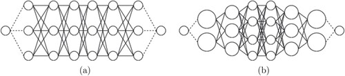
Tier i's width is denoted $|i|$. The respective diamond topology has m tiers, such that $\begin{array}{rl}\left|\lceil \frac{m}{2}\rceil \right|=\left|\lfloor \frac{m}{2}+1\rfloor \right|& =max\{|i|:i\in \{1,\dots ,m\left\}\right\},\\ |m|=|1|& =min\{|i|:i\in \{1,\dots ,m\left\}\right\}\end{array}$and, denoting $〈X〉$ as the mean of any set X, $\begin{array}{rl}& 〈\{|i|:i\in \{1,\dots ,\lceil \frac{m}{2}\rceil \}\}〉\\ & =〈\{|i|:i\in \{\lfloor \frac{m}{2}+1\rfloor ,\dots ,m\}\}〉=n.\end{array}$

Tier 1 firms represent OEMs, and firms at tier m are the Raw Materials Suppliers (RMSs). OEMs have an associated dummy consumer market node that generates demand for a number of material units and introduces it into the supply chain, such that all further demand experienced by the rest of the chain depends on this and the response by the OEM. RMSs have an associate dummy resource node, treated as having infinite resources, from which raw materials are worked to meet demand from customer firms downstream. Altogether the graph may be represented $G=(V,E)$, where $V:=\{U_i:i\in \{0,..,m+1\left\}\right\}$, $U_i$ are tiers and $|U_i|=n$.

For $i\in \{1,\dots ,m\}$, the tier, and $j\in \{1,\dots ,n\}$, the index in a single tier, firm $u_{ij}\in U_i$ stores demand at a given timestep t as $d_{ij}^t$ and have ${\iota }_{ij}^t$ inventory. OEM nodes, $u_{1j}$, receive demand from the market nodes, $u_{0j}$, according to a normal distribution with mean μ and variance ${\sigma }^2$. OEMs satisfy demand by reducing their inventory by $min\{d_{1j}^t,{\iota }_{1j}^t\}$, selling as much as they can of what the market desires, such that $\begin{array}{r}{d}_{1j}^{t+1}=d_{1j}^t-min\{d_{1j}^t,{\iota }_{1j}^t\}.\end{array}$

If $d_{ij}^{t+1}>0$, then each firm $u_{ij}\in \bigcup _{i=1}^m{U}_i$ randomly selects a connected supplier from $\{u_{i+1,k}\in U_{i+1}:(i+1,k)\in E\}$. All unfulfilled demand is backlogged, such that $\begin{array}{r}{d}_{i+1,j}^{t+1}=d_{i+1,j}^t+d_{ij}^{t+1},\end{array}$summing over all buyers that have chosen this firm. This occurs for all firms other than at tier m, the RMSs, who have no firms to pass demand onto. Instead, they increase their inventory to meet new demand such that $\begin{array}{r}{\iota }_{mj}^{t+1}={\iota }_{mj}^t+d_{mj}^t.\end{array}$

For each firm other than the OEMs at tier 1, that is, $\mathrm{\forall }{u}_{ij}\in \bigcup _{i=2}^m{U}_i$ each firm $u_{i-1,k}$ chooses a randomly connected buyer from $\{u_{i-1,k}\in U_{i-1}:(i-1,k)\in E\}$. It then ships as much material as it may send, sending out $min\{d_{ij}^{t+1},{\iota }_{ij}^{t+1}\}$, the limits of its resources and available market. This is repeated for all firms, creating a steady material flow of goods down the supply chain. To elaborate on this model, we introduce cash constraints on purchases.

4.1.2. Cash constraint extension

The above version only includes material flow; however, since there is no material acquisition limit, demand will be satisfied exactly as it enters the system, if only with market lead times of $2m$. This is because it takes m steps to reach the RMSs from the OEMs, and there is a dyadic lead time of 1.

To restrict purchases and match real conditions, we impose a cash value to purchases, stored in an edge $(u,v)\in E$, denoted $c(u,v)$. We also introduce the cash reserves of a given firm, ${\kappa }_{ij}^t$. For buyer firm u and selected supplier firm v, purchasing which is transferring a material unit in exchange for cash from v to u costs $c(u,v)$ many cash units for u and grows those reserves by the same amount for v, such that $\begin{array}{rl}& ({\iota }_u^{t+1}={\iota }_u^t+x)\\ ⟺& ({\iota }_v^{t+1}={\iota }_v^t-x)\\ ⟺& ({\kappa }_u^{t+1}={\kappa }_u^t-xc(u,v\left)\right)\\ ⟺& ({\kappa }_v^{t+1}={\kappa }_v^t+xc(u,v\left)\right).\end{array}$

We also assign a global operative cost to all firms, denoted $o_c$, which is subtracted from the cash reserves of each firm, each timestep. This has the effect of justifying the need for cash, rather than simply the desirability of profit and represents the difficulty of survival within a given supply network. The operative cost captures costs such as taxes, paying employees, rent, and is implicit of production costs, irrespective of firm size. The operative cost thus introduces restrictions which allow for complex system behaviours, but first the concept of power dynamics must be introduced, as follows.

4.1.3. Power dynamic extension

Firms in a supply network are not always equals when dealing with eachother, such that one actor in any buyer-supplier dyad may control the relationship more and have more influence than its competitors. This may be due to being a key supplier, the market-dominant brand, or having more market share. Key suppliers are nonexistent in our model since it has homogeneous material flow. We, therefore, let bargaining power be an independent parameter, corresponding to market share and access to financing, assuming that greater bargaining power suggests greater ease in negotiating bank mandates. This assumption is used to investigate the effect of varying market share for a given power position in an isolated manner.

Companies may have small, medium, or large amounts of power, represented as $s_{ij}\in \{s,m,l\}$ for all $i\in \{1,\dots ,m\}$ and $j\in \{1,\dots ,n\}$, which corresponds to access to financing.

Homogeneous material flow and companies having no unique characteristics in the model let us assume bargaining power is tied to market share. As such, a firm's power has a mapping that determines its market share, that is, how frequently it is selected among the suppliers of a buyer, such that any m or l supplier is selected, respectively, $p_m$ and $p_l$ times more than any s supplier. Using the mapping $f:s_{ij}\to \{1,p_m,p_l\}$, we have that $\begin{array}{r}\begin{array}{rl}f\left(s\right)& =1;\\ f\left(m\right)& =p_m;\\ f\left(l\right)& =p_l.\end{array}\end{array}$Defining the random variable $S_{ij}^t$ as the choice of supplier for firm $u_{ij}$ at time t, the probability mass function is $\begin{array}{rl}& \mathbb{P}(S_{ij}^t=u_{i+1,k})\\ & =\{\begin{array}{ll}{\displaystyle \frac{f\left(s_{i+1,j}\right)}{\sum _{(i+1,k)\in E}f\left(s_{i+1,k}\right)},}& (i+1,k)\in E;\\ 0,& (i+1,k)\notin E.\end{array}\end{array}$This variable dictates throughput over firms. Having a closed system with homogeneous product flow means, on average, each tier has the same total material flow. If a tier has fewer firms, then each firm has more material flow through it, resulting in greater market share in our model. To account for our linear relationship between power and market share, we define a function that, for thinner tiers, increases the company tendency to be defined as more powerful. The width of a tier is relative, such that, for a uniform random variable between 0 and 1, denoted $U(0,1)$, and for (1) $\begin{array}{r}x=\frac{U(0,1)min\left(|i|\right)}{|i|},\end{array}$(1) we have that $\begin{array}{r}{s}_{ij}=\{\begin{array}{ll}l,& x\in [2/3,1];\\ m,& x\in [1/3,2/3);\\ s,& x\in [0,1/3).\end{array}\end{array}$

Thus market share is the de-facto measure of power in this system, which is expressed in the dyads through late payments. Companies typically pay 60–120 days late (Rogers, Leuschner, and Choi 2016) for purchases, and the more powerful a company, the later it may pay to maximise its own liquidity. This is summarised in Table 1, with the delay in purchase along $(u,v)$, denoted $\delta (u,v)$, which depends on the power of the buyer, on the horizontal axis, and the supplier, on the vertical. This means that how much more powerful a buyer is than its suppliers determines how late it can pay, since they remain an important customer with a large market share.

Table 1. Table of invoice terms $(x,y)$ where agents with financing access x pay agents with financing access y after $(x,y)$ timesteps, representative of days.

	s	m	l
s	60	90	120
m	30	60	90
l	30	30	60

Using the mapping $f:\{s,m,l\}\to \mathbb{R}$ such that $f\left(s\right)=1,f\left(m\right)=2,f\left(l\right)=3$, delay is defined $\begin{array}{r}\delta (u,v)=max\left(30\right(s_u-s_v)+60,30).\end{array}$

With delayed payments, we now have a meaningful ledger of accounts payable and accounts receivable such that, given the latest a firm is meant to pay for its goods is 120 days, there is an expected inflow and outflow of cash that does not use extrapolated data. These are vectors of length 120 for each firm that change in time, denoted $P_{ij}^t$ and $R_{ij}^t$, respectively.

Using this knowledge, we can define a condition for removing a firm from the system. A firm is always operational if ${\kappa }_{ij}^t>0$ since it is currently liquid, meaning it may change its conditions by purchasing more goods to sell at profit. If ${\kappa }_{ij}^t\le 0$, then it has no liquidity, but if it expects inflows that are net positive, that is, $R_{ij}^t+P_{ij}^t>0$, then it is still a profit-making company and may continue until market conditions change; for example, competing suppliers may be removed and thus more demand will be received. If, however, ${\kappa }_{ij}^t\le 0$ and $R_{ij}^t+P_{ij}^t\le 0$ then the firm is considered unprofitable and inoperative, such that it cannot continue functioning and is removed from the network. This is not necessarily a bankruptcy, as actors within the network, in real life, may be subsidiaries of larger profitable firms. It simply means that all contractual agreements between this firm and its partners in this network are severed – for example, the firm may be absorbed into another firm in another chain, or may alter its output to become profitable.

We may also define a state of network inoperativity and thus a definition of network lifespan. If there is no route from any RMS to any OEM, then that means there is no way to bring new material goods to market. We may thus declare a network with n tiers is inactive if there does not exist any path $(u,\dots ,v)$, where u = 1 and v = n. In the $m\times n$ topologies, this means for any $k\in \{1,\dots ,n\}$, $u_{kj}\notin V$, exemplified in Figure 2.

Figure 2. Broken Lattice supply network.

Supply network graph with single nodes on the left and right, and six tiers with three nodes each in between. Tier four nodes and edges are all greyed out to represent inactivity. Nodes in adjacent tiers are all connected to eachother.

We now have a justification for a firm to find ways to remain liquid, even at the cost of profitability, which leads us to the financing extension.

4.1.4. Financing extension

A firm avoids removal from the network if it is either liquid, or expects profits. It is more valuable to have cash now than later (Benveniste, Capozza, and Seguin 2001) due to the real-life variability of conditions, competition, ability to grow in power through purchasing further assets or paying more for a more skilled workforce, and other factors. We therefore introduce a financing function that tries to stop removal for illiquidity, hypothesising that a cost to overall profits is worth the gain in current profits.

We first explore bank financing. If a firm is illiquid, that is, ${\kappa }_{ij}^t\le 0$ at the end of a timestep, then it will seek financing from a traditional bank loan. The amount of financing available, or banking mandate limit, denoted $b_{ij}^t$, is dependant on the credit worthiness of the firm, which its bargaining power allows it to negotiate.

Credit worthiness is approximated as scaling to company power and current cash, such that it is a product of a measure of power and liquidity. That is, $\begin{array}{r}{b}_{ij}^t=\{\begin{array}{ll}2{\kappa }_{ij}^t,& s_{ij}=s;\\ 3{\kappa }_{ij}^t,& s_{ij}=m;\\ 4{\kappa }_{ij}^t,& s_{ij}=l.\end{array}\end{array}$We also have a separate variable, firm debt, denoted ${\rho }_{ij}^t$, that refers to the size of the overall debts owed by a given firm, including interest, that has not yet been repaid. If ${\rho }_{ij}^t\ge b_{ij}^t$ then a firm cannot incur more debt. This is another expression of a power disparity – greater market control gives greater freedom to remain illiquid for longer. Denoting available BF as ${\text{β}}_{ij}^t$, the function is such that $\begin{array}{r}{\text{β}}_{ij}^t=max(min(b_{ij}^t-{\rho }_{ij}^t,\left|{\kappa }_{ij}^t\right|),0)\end{array}$then, denoting our existing ${\kappa }_{ij}^t$ as ${\kappa }_{ij}^{\mathrm{\prime }t}$ then we can update ${\kappa }_{ij}^t$ such that $\begin{array}{r}{\kappa }_{ij}^t={\kappa }_{ij}^{\mathrm{\prime }t}+{\text{β}}_{ij}^t.\end{array}$This manner of appending variables with a ‘prime’ is used in this paper to denote the same variable during an operation within a timestep. As an approximation of fixed loan repayments over the long term, we assume all interest is paid by the longest date into the future our model takes – 120 days. We denote the annual interest rate for bank loans as $i_b$, such that $\begin{array}{rl}{P}_{ij}^{t+120}& =P_{ij}^t+{\text{β}}_{ij}^t\cdot i_b/365\cdot 120;\\ {\rho }_{ij}^t& ={\rho }_{ij}^{\mathrm{\prime }t}+{\text{β}}_{ij}^t\cdot i_b/365\cdot 120.\end{array}$

Thus, there are cases when the banking function does not provide sufficient funds to be liquid. To solve this issue of inaccessible bank financing, we introduce supply chain financing. We model supply chain financing that comes from alternative sources that allow for focal firms with neither a monopoly nor a stable market. In this case, invoices are sold at some discount in exchange for immediate liquidity, moving a discounted amount of accounts payable from a given invoice term from the future to the present. We give a global term, denoted τ, that is a parameter defining the number of timesteps into the future we reduce accounts payable from. Instead of being restricted by $b_{ij}^t$, available supply chain financing, denoted ${\xi }_{ij}^t$, is restricted by $R_{ij}^{t+\tau }$, such that $\begin{array}{r}{\xi }_{ij}^t=max(min(\left|{\kappa }_{ij}^t\right|,R_{ij}^{t+\tau }-\left|{\kappa }_{ij}^t\right|),0).\end{array}$Then we have $\begin{array}{r}{\kappa }_{ij}^t={\kappa }_{ij}^{\mathrm{\prime }t}+{\xi }_{ij}^t.\end{array}$

We assume interest is paid at the invoice due date, such that we remove the size of the invoice from the accounts receivable, and add the size of the interest, an annual rate of $i_s$ to the accounts payable. This is defined as: $\begin{array}{rl}{P}_{ij}^{t+\tau }& =P_{ij}^{\mathrm{\prime }t+\tau }+{\xi }_{ij}^t\cdot i_s/365\cdot \tau ;\\ R_{ij}^{t+\tau }& =R_{ij}^{\mathrm{\prime }t+\tau }-{\xi }_{ij}^t.\end{array}$

With these we have functions that mitigate versus failure within the network, using financing. However, firms have ways to estimate their future earnings and demand based on previous behaviour, and from there we can estimate their financing requirement. Therefore, we move onto a proactive extension of the financing functions, rather than reactive.

4.1.5. Proactivity

We can estimate incoming costs by computing a moving average of demand and multiplying this by the average purchase cost among suppliers. We use an iterative computation to estimate the moving average thus avoiding any information storage. We define cash requirements, $r_{ij}^t$, such that $\begin{array}{r}{r}_{ij}^t=max(0,d_{ij}^t〈\left\{c\right(u_{ij},v):(u_{ij},v)\in E\}〉),\end{array}$then include a global window size parameter, w, that determines widths of moving average windows. We then define the moving costs average $\overline{c_{ij}^t}$ recursively, such that $\begin{array}{r}\overline{c_{ij}^t}=\{\begin{array}{ll}{r}_{ij}^t,& t=1;\\ \left(\overline{c_{ij}^{t-1}}\right(t-1)+r_{ij}^t)/t& t\le w;\\ \left(\overline{c_{ij}^{t-1}}\right(w-1)+r_{ij}^t)/w& t>w.\end{array}\end{array}$We now have a dynamic estimate of the required cash to meet demands at any given moment. This can be used as a proactive threshold, giving us two cases for each financing method, that of reactive BF, proactive BF, reactive SCF (analogous to invoice discounting from firms seeking alternative financing), and proactive SCF (analogous to reverse factoring from contractual agreements with supply chain financing firms).

Proactivity makes financing happen sooner, reducing profits due to the interest incurred, $i_b$ and $i_s$. As a reward for proactivity and seeking financing while the company still has resources, let us say the annualised interest rates are $1\mathrm{\%}$ less than they would be if reactive. This means if ${\kappa }_{ij}^t\le \overline{c_{ij}^t}$, then for proactive banking, $\begin{array}{rl}{\text{β}}_{ij}^t& =max(min(b_{ij}^t-{\rho }_{ij}^t,\overline{c_{ij}^t}-{\kappa }_{ij}^t),0);\\ P_{ij}^{t+120}& =P_{ij}^t+{\text{β}}_{ij}^t\cdot (i_b-0.01)/365\cdot 120;\\ {\rho }_{ij}^t& ={\rho }_{ij}^{\mathrm{\prime }t}+{\text{β}}_{ij}^t\cdot (i_b-0.01)/365\cdot 120\end{array}$and for reverse factoring, $\begin{array}{r}{P}_{ij}^{t+\tau }=P_{ij}^{\mathrm{\prime }t+\tau }+{\xi }_{ij}^t\cdot (i_s-0.01)/365\cdot \tau .\end{array}$

This concludes the simulation methodology. Our analytical methodology is outlined in the following subsection.

4.2. Analytical methodology

We run repeated simulations across a spectrum of model parameters, exploring a wide selection of the experimental space, analysing the lattice and diamond topologies. We assume demand is independently identically normally distributed for each market node.

We first analyse the relative significance of different parameters upon the survivability of the supply network and constituent company types by determining the theoretical distribution of company types per topology, then measuring the deviation from this distribution.

Our null hypothesis is the theoretical distribution of generated companies, Q, equals the empirical distribution of failures per company type, P. Our alternative hypothesis is topology affects the failure distribution, such that $Q\ne P$. This is determined by calculating Kullbach-Liebler divergence (Kullback and Leibler 1951), denoted $D_{\mathrm{K}\mathrm{L}}$, between P and Q. For the state space of the proportion of company failures by bargaining power, X, we define $D_{\mathrm{K}\mathrm{L}}$ as $\begin{array}{r}{D}_{\mathrm{K}\mathrm{L}}\left(P||Q\right)=\sum _{x\in X}P\left(x\right)\log \left(\frac{P\left(x\right)}{Q\left(x\right)}\right).\end{array}$

Let the number of failures on the $i^{th}$ simulation for small (s), medium (m), and large (l) companies be denoted, respectively, $s_i,m_i,l_i\in \mathbb{N}$. These sum to the total company failures in simulation run i, $R_i=s_i+m_i+l_i$, which sums to the total number of failures, $R=\sum _i{R}_i$.

Simulation parameters are varied deterministically, but by treating simulations as a sample, relative risk can be calculated in two ways. First is in aggregate, finding the proportion of failures over all simulations, denoting aggregate P as $P_a$, such that, for $x\in (s,m,l)$, and $x_i$ as the failure count of a given company type at simulation i, $\begin{array}{r}\mathbb{P}(P_a=x)=\frac{\sum _i{x}_i}{R}.\end{array}$Second is piecewise, finding the proportion of failures per simulation, summing together proportions, then dividing by total likelihood. We denote piecewise P as $P_p$, giving $\begin{array}{r}\mathbb{P}(P_p=x)=\frac{\sum _i\left(\frac{x_i}{R_i}\right)}{\sum _i(\frac{s_i}{R_i}+\frac{m_i}{R_i}+\frac{l_i}{R_i})}.\end{array}$

$D_{\mathrm{K}\mathrm{L}}$ is then calculated for $P_a$ and $P_p$ versus the theoretically generated company types. $D_{\mathrm{K}\mathrm{L}}$ is useful for analysing significance and difference but gives no insight into the nature of distribution. For that, we directly study the histograms of failure and fit probability distribution curves to them.

For systemic analysis, we use Kernel Density Estimates (KDEs) (Parzen 1962; Rosenblatt 1956) over the systemic survival times histograms to produce curve fittings for inspection. Since KDEs showed multiple inflection points, we also fit unimodal Gamma and bimodal Gaussian mixture distributions (Reynolds 2009) for the system survival times.

Our model mitigates against ripple effects using financing. We explore the effect of varying parameters associated with financing, including interest rates, repayment term times for supply chain financing, and whether financing is proactive or reactive. With reactive financing, companies seek financing whenever they have zero liquid cash. With proactive financing, a company, before it has zero liquid cash, predicts future cash flows with a moving average window to determine a dynamic threshold, below which it seeks financing. We also investigate the effect of adjusting window length.

We examine system and company survivability. Our model may heterogeneously distribute access to financing, and thus associated financing function, or treat all companies homogeneously. We conduct a moderated regression analysis with p = 0.05 as a significance threshold of parameters governing the financing. Regression analysis is further broken down by moderating whether the system is financed and under which paradigm.

5. Results

Experiments were conducted over the space of model parameters in Table 2. Simulations were completed on an Armari Magnetar workstation, with a 3.5GHz Intel Xeon E5-1620 CPU, 64GB RAM, in Windows 10 Pro. Modelling and results were completed in Python 3 with the math, random, csv, itertools, os, numpy, statistics, matplotlib, pandas, seaborn, fitter, and scipy libraries.

Table 2. Table of the parameters tested.

Parameter	Values
Operation Fees	5, 10, 15
Average Demand	5, 20, 50, 100
Demand Standard Deviation	5, 10, 15
Company Power Distribution	Homogeneous, Heterogeneous
Financed	True, False
Paradigm	Reactive, Proactive
Supply Chain Financing Annual Rates	1.01, 1.03, 1.05, 1.07, 1.09, 1.20, 1.50, 2
Bank Annual Rates	1.01, 1.03, 1.05, 1.07, 1.09, 1.20, 1.50, 2
Terms	5, 30, 60, 90, 120
Window Sizes	5, 30, 60, 90, 120
Medium Power Market Share	1, 2, 5
Large Power Market Share${}^{\mathrm{a}}$	1, 3, 10, 20
Topologies	Lattice, Diamond

${}^{\mathrm{a}}$Large power market shares that would be smaller than medium power market shares are not tested

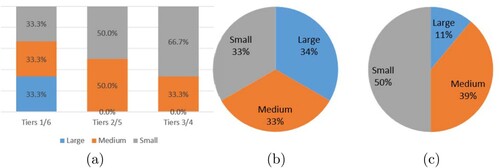
We investigate the topologies in Figure 1(a and b). Upon generation, power is distributed in the lattice equally across tiers and through the network as in Figure 3(b), and in the diamond, as a result of Equation (1(1) $\begin{array}{r}x=\frac{U(0,1)min\left(|i|\right)}{|i|},\end{array}$(1) ), is distributed according to Figure 3(a), resulting in Figure 3(c).

Figure 3. Distributions of company powers upon generation of a network topology of a given type. Since the diamond topology is heterogeneous, we also show the distribution per tier. (a) Diamond topology power distribution per tier. (b) Whole network power distribution in lattice topology.

(a) Stacked bar charts of the distribution of power per tier. Tiers 1 and 6 have 1/3 for large, medium, and small power each, tiers 2 and 5 have 1/2 for medium and small each, tiers 3 and 4 have 2/3 for small and 1/3 for medium. (b) Pie chart of power distributions across the lattice topology. 1/3 for each of small, medium, and large power companies. (c) Whole network power distribution in diamond topology. (c) Pie chart of power distributions across the diamond topology. 50% for small, 39% for medium, and 11% for large power companies.

To understand the relative risk incurred upon a company with given bargaining power, we compare the distributions of generated companies to that of failed companies by looking at distributions in aggregate (Figure 4(a and c)), then piecewise by averaging proportions of failures for each simulation run (Figure 4(b and d)). Next, we calculate the $D_{\mathrm{K}\mathrm{L}}$ between theoretical distributions of generated companies and empirical distributions of company failures (Table 3). We then inspect the histograms in Figure 5 and fit probability distributions to them (Table 4). Table 5 captures mean days survived of each company type under each topology.

Figure 4. Distribution of power among company failures in lattice and diamond topologies, as well as in total or piecewise. (a) Lattice topology aggregate failure distribution. (b) Lattice topology piecewise failure distribution. (c) Diamond topology aggregate failure distribution. (d) Diamond topology piecewise failure distribution.

(a) Pie chart of power distributions across the diamond topology. 30% for small, 34% for medium, and 36% for large power companies. (b) Pie chart of power distributions across the diamond topology. 21% for small, 32% for medium, and 47% for large power companies. (c) Pie chart of power distributions across the diamond topology. 36% for small, 36% for medium, and 28% for large power companies. (d) Pie chart of power distributions across the diamond topology. 43% for small, 37% for medium, and 20% for large power companies.

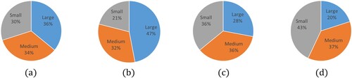
Figure 5. Histograms of company survival times divided by topology and company type, with fitted curves. Survival time is in days. (a) Small company survival times on a lattice; (b) Medium company survival times on a lattice; (c) Large company survival times on a lattice; (d) Small company survival times on a diamond; (e) Medium company survival times on a diamond; (f) Large company survival times on a diamond; (g) Homog. company survival times on a lattice and (h) Homog. company survival times on a diamond.

Histograms of company survival times in blue, with fitted curves of the histograms superimposed in grey and red. Red curves are the most accurate, and their distribution type is shown in the legend. The mean of the histograms is also superimposed on the graph with a dashed vertical line at its position.

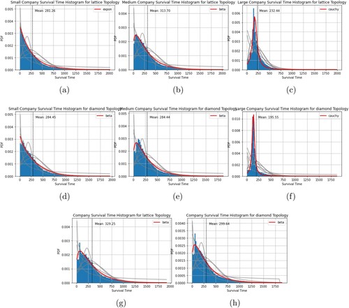
Table 3. Difference in failures to generated companies.

	KL divergence	Small difference	Medium difference	Large difference
Lattice Aggregate	0.04897	−3%	1%	2%
Lattice Piecewise	0.4078	−12%	−1%	13%
Diamond Aggregate	0.1094	−14%	−3%	17%
Diamond Piecewise	0.0361	−7%	−2%	9%

Table 4. Fitted probability distributions of company survival time histograms for each company type. Time is in days.

	Topology
Company Type	Lattice	Diamond
Homog. Company	Beta $(\alpha =1.27,\text{β}=58.9)$	Beta $(\alpha =1.24,\text{β}=1.29\mathrm{e}5)$
Small Company	Exp $(\mu =280)$	Beta $(\alpha =0.97,\text{β}=7.28)$
Medium Company	Beta $(\alpha =1.21,\text{β}=1.56$e$8)$	Beta $(\alpha =1.26,\text{β}=2.05$e$11)$
Large Company	Cauchy $(x_0=174,\gamma =56.6)$	Cauchy $(x_0=134,\gamma =27.9)$

Table 5. Mean number of days survived for a given company type in a given topology.

	Company type
Topology	Homog. Company	Small	Medium	Large
Lattice	329.25	281.26	313.70	232.44
Diamond	299.64	284.45	284.44	195.55

Then we fit unimodal Gamma distributions and bimodal Gaussian mixture model distributions over the histograms of systemic survival times of lattice and diamond networks (Figure 6). KDEs are shown in Figure 7. Relative accuracy of the unimodal and multimodal distributions was compared using residual sums of squares (RSS) (Table 6). Moderated regression analysis for each dependant term is summarised in Table 7.

Figure 6. Histograms of system survival times divided by topology, with fitted bimodal gaussian mixture curves. W is a unimodal Gamma distribution, which was found to be the most accurate of the tested unimodal distributions. $X_1$ and $X_2$ are the first and second Gaussians, with associated means ${\mu }_1$ and ${\mu }_2$, and variances ${\sigma }_1^2$ and ${\sigma }_2^2$, respectively. Y is the mixture distribution using $X_1$ and $X_2$. (a) System survival times on a lattice and (b) System survival times on a diamond.

Histograms of company survival times in blue, with fitted curves of the histograms superimposed on top. The thin red curves are the unimodal gamma distribution. The thick pink and green curves are, respectively, the first- and second-fitted Gaussians. The thick black curves are the fitted mixture distributions. The legend contains curve parameters. The mean of the histograms is also superimposed on the graph with a dashed vertical line at its position.

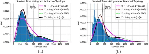
Figure 7. Kernel density estimates of system survival times for lattice and diamond topologies in days. (a) KDE of system survival times on a lattice and (b) KDE of system survival times on a diamond.

Curves of KDEs for the lattice and the diamond topologies in dark blue bounding from above an area of faded blue.

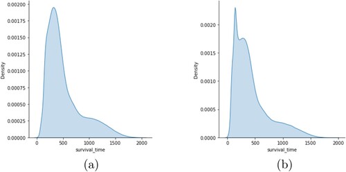
Table 6. Residual sums of squares (RSS) of Gamma and Gaussian Mixture Model (GMM) distribution fit for both lattice and diamond topologies.

	RSS
Topology	Gamma	GMM
Lattice	7.60e-6	3.68e-6
Diamond	7.71e-6	1.20e-5

Table 7. Table of moderated regression coefficients, assuming a system with financing.

			Regression Coefficient
				Annualised Interest Rates
Network Object	Topology	Paradigm	Supply Chain Financing Product Terms	Supply Chain	Bank	Proactivity Window
System	Lattice	Reactive	*	*	*	x
System	Lattice	Proactive	−2.53	*	*	*
System	Diamond	Reactive	*	0.53	*	x
System	Diamond	Proactive	−3.2	0.54	*	−0.01
All Companies	Lattice	Reactive	*	−0.19	*	x
All Companies	Lattice	Proactive	−2.57	−0.09	−0.72	−0.01
All Companies	Diamond	Reactive	*	0.17	−1.09	x
All Companies	Diamond	Proactive	−3.21	0.18	*	−0.01
All Heterogeneous Companies	Lattice	Reactive	*	−0.14	−0.83	x
All Heterogeneous Companies	Lattice	Proactive	−2.7	−0.15	*	−0.02
All Heterogeneous Companies	Diamond	Reactive	*	0.3	−1.02	x
All Heterogeneous Companies	Diamond	Proactive	−3.24	0.18	*	−0.01
All Homogeneous Companies	Lattice	Reactive	*	−0.19	*	x
All Homogeneous Companies	Lattice	Proactive	−2.36	−0.13	*	*
All Homogeneous Companies	Diamond	Reactive	*	0.07	−1.35	x
All Homogeneous Companies	Diamond	Proactive	−3.11	0.15	*	−0.01
Large Companies	Lattice	Reactive	*	−0.51	*	x
Large Companies	Lattice	Proactive	−2.1	−0.54	*	−0.01
Large Companies	Diamond	Reactive	*	*	*	x
Large Companies	Diamond	Proactive	*	*	*	*
Medium Companies	Lattice	Reactive	*	0.2	*	x
Medium Companies	Lattice	Proactive	−3.47	0.28	*	−0.02
Medium Companies	Diamond	Reactive	*	*	*	x
Medium Companies	Diamond	Proactive	*	*	*	−0.01
Small Companies	Lattice	Reactive	*	0.36	*	x
Small Companies	Lattice	Proactive	−3.05	0.34	*	−0.04
Small Companies	Diamond	Reactive	*	0.49	*	x
Small Companies	Diamond	Proactive	−3.71	0.3	*	−0.02

‘-’ means the p-value of the variable in question for that configuration is below 0.05. ‘x’ means that the variable in question is degenerate for that configuration.

6. Discussion

In this paper, we created a supply network simulation model where selfish actors with different degrees of bargaining power try to maximise their liquidity by negotiating longer repayment terms and other financing functions. We study the resultant financial ripple effects using survivability analysis.

We first address the use of bargaining power in this model. Companies are distinguished by power category, which endows them with the capacity to set terms. A real company may then choose to have smaller BF mandates and pay invoices sooner, but if a firm decides it needs financing, for it to be a logical actor, it must choose to set terms that maximise the availability of financing at minimum rates. Similarly, since later payments mean higher liquidity, if firms are selfish, then it logically follows more power means longer repayment schedules and larger mandates. Therefore, companies have small, medium, and large amounts of bargaining power, which is coupled with access to financing and repayment times. This follows existing power or size classifications, such as the concept of small, medium, and large enterprises.

Using the bargaining power argument, we investigate if topology significantly redistributes risk according to bargaining power. Since greater bargaining power yields greater access to BF, this gives us a measure of the risk trade-off in return for superior financing.

6.1. Company level

In Table 3, small power company risk is always overestimated in generation, with $3\mathrm{\%}$ to $14\mathrm{\%}$ fewer failures empirically. Medium power companies have a $-3\mathrm{\%}$ to $1\mathrm{\%}$ difference empirically, suggesting predictions are accurate for them. Large power companies are underestimated, with $2\mathrm{\%}$ to $17\mathrm{\%}$ more empirical failures, scaling with the overestimation of small failures. This suggests that in exchange for greater power, large companies absorb risk from smaller companies, perhaps due to greater market exposure, where in our case, industrial effects are stronger than firm strengths, as in Fernández et al. (2019), though this must be investigated further. Additionally, company creation may be a misleading systemic risk measure, since it overestimates risk to small companies but underestimates risk to large ones, which have more impact. Measures of reduced operation, such as failure, are needed for accurate measurement (Acharya et al. 2017).

Risk is predicted accurately by generation on the lattice in aggregate where $D_{\mathrm{K}\mathrm{L}}<0.05$. Piecewise for the lattice, however, has a $D_{\mathrm{K}\mathrm{L}}>0.4$, such that generation does not predict risk. In the diamond, the risk is not predicted by generation in aggregate, where $D_{\mathrm{K}\mathrm{L}}>0.1$, but is predicted piecewise, where $D_{\mathrm{K}\mathrm{L}}<0.04$. The lattice is the base case, with homogeneous tiers, while the diamond is deep tier, with structured topology and heterogeneous tiers. Failures aggregation closely matches theoretical generation, suggesting configuration does not change the shape of the distributions from generation, but drastically changes number of failures, captured by piecewise measurement. This may be due to the linearity of the lattice, manifesting in linear changes. Diamond topology aggregation analysis is significant, put piecewise is not, suggesting configuration affects the number of failures in a run, but not the distribution. This may be because of the overriding influence of the deep-tier topology, where medium firms tend to connect to both small and large ones, and their stronger relationship with industry structure affects the rest of the system (Fernández et al. 2019).

Homogeneous company failures (Figure 5(g and h)) are beta distributed for both the lattice and diamond. The diamond has less deviation with a smaller scale parameter of $\text{β}=1.29$e5 versus the lattice's $\text{β}=58.9$ (Table 4). Both have similar shape parameters ($\alpha =1.27$ and $\alpha =1.24$ for the lattice and diamond, respectively), suggesting homogeneous company failure distribution is resistant to topology. This follows the right skewness of graphs of failures versus age in Kücher et al. (2020), though at a smaller timescale. While a timestep is interpreted as a day in our model, it is in truth an arbitrary restocking period so result on survival time are applicable at all timescales.

Small companies in the lattice (Figure 5(a)) are exponentially distributed, centred around 0 days with exponential decay. In the diamond, they formally fit to a beta distribution, also centred around 0, following approximately the same shape as the exponential curve (Figure 5(d)), suggesting small company failures are generally exponentially distributed.

Medium companies are beta distributed, which is not necessarily symmetric, capturing their skewed failure distributions (Figure 5(b and e)). Shape parameters in the lattice and diamond are $\alpha =1.21$ and $\alpha =1.26$, respectively, with smaller scale for the diamond. Medium shape parameters match those for homogeneous companies suggesting medium companies most characterise company survival.

Large companies are Cauchy distributed. This suggests failures for large companies are symmetric but shifted down (Figure 5(c and f)). This could be an artefact of the long large company failure tails which match the Cauchy distribution.

Respective modes of company survival times suggest the first companies to fail are small, then medium, then large. Large companies have the worst mean survival time, while homogeneous companies are top performers. Small, medium, and homogeneous companies have fat tails, while large ones have thin tails, meaning the system has adapted such that large companies fail quickly. Since only medium firms empirically have been found to be more affected by the supply chain or industry than their own firm attributes, this suggests exceptional integration between firms in the supply chain. Further analyses on more sparsely connected or purely empirical graphs should be explored. Our model also, therefore, suggests greater financing for companies with greater bargaining power means more debt, which reduces overall cash reserves. Due to the greater risk exposure caused by dependence on more weak companies, this results in a misuse of funds, since partner risk is not considered in financing. Future work may investigate if stronger awareness of deep-tier partners, used to calculate available financing, will reduce relative risk exposures of focal companies and increase system survival time.

We also find that company survival times are worse in the diamond than in the lattice (Table 5). We propose the diamond has a higher risk exposure because stronger companies are positioned closer to the market and raw materials supplier in thinner tiers, thus relying on a larger number of weaker companies, who in turn suffer from less liquidity because these powerful companies are paying late too often. This highlights the combination of bullwhip effects and financial ripple effect in action Li et al. (2021). As inefficient weaker companies get eliminated, prior systemic adaptations now mean such poor market conditions that previously strong companies fail in quick succession. This results in thinner tails, such that there are fewer very well-performing network configurations. This may be because of the bias to certain configurations introduced by the tier-dependent company power selection. Future work may study the burstiness (Neuts 1993) of failures to evidence this.

Altogether, we have that:

• greater bargaining power for buying firms and its benefits are achieved by greater risk exposure;

• the extended diamond topology is generally worse for company survival than a lattice;

• skew of risk to powerful companies is greater in the diamond than in the lattice;

• powerful firms should protect weaker ones in their supply chain to prevent their own failure;

• both deep-tier SCF and BF without considering partner exposure may result in inefficiencies;

• homogeneous configurations are resistant to the negative effects of the diamond topology but still perform better in the lattice as well.

These results combined suggest to us that increased heterogeneity in both topology and characteristic powers, while improving the relative survivability of larger companies since they fail after small ones, overall reduces systemic survivability. Since large companies fail after small ones, this may explain the large company risk skew – their advantages undermine the system, who's survival dominates theirs. Thus focal company supply chain managers should both seek to uplift the cash positions and promote the growth of their suppliers to improve their own and minimise predatory tactics of later payments. This closely follows existing literature (Rogers, Leuschner, and Choi 2020), but that the results hold at a complex systems level further reinforces them as essential for the long-term resilience of supply chains. Organising supply chain financing via reverse factoring is one way to satisfy both the liquidity requirements of focal firms and suppliers, though care must be taken that financing remains accessible to all members of the chain in equal measure.

Having analysed company survivability and observed how these affect systemic survivability, we now examine the survivability of the system itself.

6.2. System level

Inspecting KDEs of histograms in Figure 7, we see multimodality via multiple inflection points for both lattice and diamond topologies. We, therefore, conduct our analysis with the Gaussian Mixture Model (GMM) in mind.

The first mode of the lattice network is approximately 300 to 350 days, matching the mean of lattice company survival times (Figure 6(a)). This is true for diamond system survival, modal at approximately 150 to 300 days, or 250 to 300 days, not counting the failure spike matching the company survival times in the diamond topology (Figure 6(b)), clear since large firms occupy thinner tiers (Figure 5(c and f)). Bimodality suggests system survival times may be distributed differently after mean focal company failure times versus those before. Further analysis may be needed to investigate this.

To prove multimodality, we compared the GMM to the best performing unimodal distribution, found similar to the distributions in Table 2. This is a gamma distribution, likely owing to the irregular skew of system survival times (Table 1). RSS were calculated to determine relative distribution accuracy (Table 6). The GMM and gamma distributions represent the lattice topology better than they do the diamond. The lattice GMM outperforms the gamma, with RSS 3.68e-6 and 7.60e-6, respectively. The diamond GMM performs worse than the gamma, with RSS 1.20e-5 and 7.71e-6, respectively. We propose this is due to the high density of early systemic deaths. The GMM performed well overall, suggesting bimodality is correct, if not ideal for curve fitting.

Looking at the $X_1$ normal curves (Figure 6(a and b)), we see mean survival time is ${\sigma }_1$ above ${\mu }_1$, while the $X_1$ and $X_2$ intercept is around $2{\sigma }_1$ above ${\mu }_1$, and ${\sigma }_2$ below ${\mu }_2$. This gives us a basic topology of the survivability space and what a given simulation's survival time suggests about the stability of a supply network.

The survival space has a wide range. To understand this further and explore the survivability space, we conduct a moderated regression analysis of the mitigating functions and their variables in this model.

6.2.1. Mitigation of ripple effects

This subsection examines regression coefficients of a moderated regression analysis of a spread of mitigation function parameters (Table 7). Operation fees, average market demand, and demand standard deviation always significantly change the survivability of any network object under all other parameter combinations, so they are the primary drivers of the simulation model. Interest rates for SCF and BF, and repayment terms for SCF depend on there being financing. The window to inform the proactive financing threshold depends on financing being proactive. We , therefore, restrict moderation to network object, topology, and financing paradigm.

6.2.1.1 Supply chain financing product term

Term is the length of time after which SCF products are repaid. Term only has significant impact in the proactive financing case despite not being degenerate for reactive financing. When it is significant, we find longer terms of repayment for invoices tend to have the largest impact on survivability. This suggests shorter terms promote survivability only for companies with predictive ability. Under proactive financing, term has significant impact on survival time for all lattice network objects. In the diamond, term under a proactive paradigm is significant for all expect medium and large companies, who survive independent of term.

In reactive systems, all functions depend on cash available within the system at the present time. Greater delays in repayment do not directly change total cash, but they do change its distribution. We conclude that predictive functions depend on distribution of cash, and more specifically, work better when there is a stronger coupling between material and cash flows. Longer terms also mean larger fees upon repayment, overall reducing total system cash, so managers should make sure to avoid increasing their liquidity as much as possible through late payments, while policymakers may wish to deliver incentives for earlier payments to allow for this.

6.2.1.2 Supply chain financing interest rates

Higher interest rates positively correlate with diamond topology system survival time and all small company survival times but are insignificant for medium and large companies. Higher rates have positive impact for the ‘all companies’ category in a diamond topology, but negative impact in the lattice topology. Large companies are negatively impacted by higher rates in the lattice. Together, this suggests that system survival time, as a function of supply chain interest rates, is driven by large companies. When the negative effects of higher rates are insignificant for large companies, however, small company survival time dominates as the system survival driver, which is improved by higher rates. In the topologically homogeneous lattice, higher rates simply impose more restrictions on the whole system. In the topologically heterogeneous diamond, large companies are more dependent on their supply chain than any financing functions. In this case there is less survival time variation (Figures 5 and 6), and a tendency for earlier system failure (Figure 6(b)), suggesting fewer viable configurations. We propose that higher rates eliminate companies in inefficient positions within the system, bringing more business to small nexuses, achieving more stable configurations sooner. This is a consequence of the adaptivity of the model.

Upon initialising a simulation, longer terms give a longer grace period to ill-configured firms. Increasing terms reduces total system cash but extends the period of inefficient configuration of the model. This leads to smaller cashflows to otherwise efficient companies, thus uniformly reducing survivability. Increased SCF rates give no such grace period.

Policymakers may take notice that higher rates for alternative financing may actually improve supply chain resilience in supply ecosystems where tiers are highly asymmetric. Supply chain managers may work together with policymakers to support them in increasing tier flexibility by adding new suppliers and buyers at tiers with few options to protect their supply chain and keep financing widely accessible.

6.2.1.3 Bank financing interest rates

BF interest rate has either a negative regression coefficient or is insignificant. Both system survival time and survival time of particular company types are unaffected by changing BF interest rates. We propose this is due to the structure of repayment within the model; companies need only pay back cash 120 days into the future rather than the shorter terms typical of SCF. As the repayment date is past the most common removal time of any company, nodes do not feel the effects of repaying BF.

Increasing BF interest rates, unlike increasing SCF interest rates, always negatively affects survival times when it is significant. It may be that financing is only repaid after the network has settled into a reliable topology. If it had effect before stabilisation of the supply chain, then it would have the option to help remove inefficient companies. However, since it always has negative effects for increased rates, we conclude it is only affecting efficient companies.

This may suggest that for low-growth supply ecosystems with high interchange ability, from the model perspective, high bank loan interest rates reduce survivability, so policymakers should try to either induce the creation of more key suppliers and economic growth through the support of disruptive technology (Christensen, Craig, and Hart 2001) or suppress bank rates, possibly with reduced regulation (Buchak et al. 2017).

6.2.1.4 Proactivity window

The moving average, or proactivity window, has the smallest impact of all mitigation factors, ranging from −0.04 to −0.01, and is always negative. It has no impact on survival for lattice systems, homogeneous lattice companies, and large diamond companies. It significantly affects survivability for all other moderated tests.

The regression coefficient is small because changing the proactivity window does not change actual flows, it skews the financing threshold to older information. Information used in a shorter proactivity window is always contained within a longer one, so the relative amount of new information decreases as the window length used increases. This means that, as long as the threshold changes linearly with the window, there is little scope for change. The ranges for which new information contributes meaningfully to the threshold are small and close to the present time, so deviate only a small amount from the threshold derived from smaller windows.

Managers must engage in some degree of predictive behaviours to optimise profits, but evidence shown here suggests that limited solutions can actually be detrimental. Managers must ensure that they are interpreting data correctly, which would be aided by greater data sharing and communication between partner firms, and greater investment in supply analytics.

6.2.1.5 Moderated regression analysis summary

Not all mitigation function parameters are significant. The most impactful parameter is the length of supply chain financing (SCF) repayment term, with a consistently negative regression coefficient. Second is the interest rate for bank financing, meaningful for reactive systems. Third is the SCF interest rate, significant for most configurations. The least significant is proactivity window length, always negative. Key observations on each parameter are:

• minimising time to repayment of SCF products should improve survivability of the system and supply chain participants;

• higher SCF interest rates may remove inefficiently distributed companies, producing a positive effect on system survivability and network participants;

• higher bank financing (BF) interest rates do not affect most network objects under most conditions, and most likely only affect efficient and otherwise stable systems. Hence, they may work as a useful financing source in stress periods if available;

• the width of the proactivity window has little effect, and only negative, so a more advanced and nonlinear method of processing past information is necessary to study this relationship.

Finally, regression coefficients for mitigation functions are often unintuitive or insignificant. We propose that this is a consequence of the model being both closed and non-evolutionary. It is closed since the supply chains investigated do not affect external systems that influence the supply chain itself – they are assumed to function independent of the supply chain. It is non-evolutionary since there is no growth function of firms or the supply chain. The function of financing is to allow growth to the point of profitability through the stages of unprofitability. Since this system only exhibits adaptivity through rewiring upon failure, financing can only be used to carry a system through to stability after cutting off inefficiencies. This limitation has the benefit of ensuring failure after a certain time, allowing for survivability analysis of the sort conducted here, however, further research should incorporate growth functions and external relationships to better emulate the use of financing.

7. Conclusions

To investigate the financial ripple effect (FRE) on supply networks, we created a simulation model of a complex adaptive supply network with financing, where companies vary repayment schedules, generating financial squeeze which in turn causes disruptions. This is an agent-based supply network simulation model with homogeneous material flow, cash-constrained transactions where companies are differentiated by their negotiating power, which affects their access to financing and how late they may pay for purchased goods. In the system, companies seek financing to fill the liquidity gap caused by delayed payments, and financing can be sought out proactively ahead of expected financial ripples using estimates of future demand. Companies are removed from the system whenever they run out of cash, whereupon buyers switch to sourcing from alternative suppliers. In modelling this, we capture the decay effects of a reconfigurable supply chain (Dolgui, Ivanov, and Sokolov 2020).

Tests were completed using two characteristic supply network topologies: a lattice, with homogeneous tiers; and an extended diamond, with heterogeneous tiers and deep-tier structure. A moderated regression analysis was conducted to analyse parameters that govern financing, designed to mitigate against FREs.

In studying this using a complex adaptive system as a network, we are able to observe the relationship between agent properties and system resilience. Results on the relationship between predictive methods and information gathering in this context can also be used to inform when and how to construct supply chain digital twins or any other representative models for maximising resilience and viability.

Policy makers should also note that increased visibility of supply chain structure is important to attain, as our study shows that topology has a significant impact on financial resilience.

We found that powerful companies tend to be overexposed to risk, over-represented in the number of failures they experience. Results suggest this is because less powerful companies fail first, turning the network topology unstable, whereupon powerful firms fail in quick succession before complete system failure. This suggests firms with more power should support weaker firms to prevent a failure cascade.

From our company survivability analysis, we found that the diamond topology is worse for company survival time than the lattice. We propose this is due to increased partner risk, which financing functions do not consider. Thinner tails suggest that greater heterogeneity limits configurations that can survive in the long term and results suggest homogenising company bargaining powers to ensure this.

Our system survivability analysis shows the diamond topology is also worse for system survival than the lattice. This suggests that deep-tier structure, when not correctly accounted for, is detrimental to survival. We also found that survival may be distributed bimodally, suggesting there may be a categorical difference in resilience between some configurations and others.

Using moderated regression analysis on system survivability, we found the following:

Longer repayment terms for SCF products in a closed system only negatively impact survivability for all network objects when a prediction function is in place (as it is likely to be in reality) else it has no impact.

Liquidity, within this closed system, appears to be less valuable than total cash. We, therefore, suggest that invoice terms should be minimised to improve member survivability in a supply chain.

Conditioned on size, only small companies depend on term times with the largest coefficient magnitude of all tested. Large and medium companies are affected only by terms in the lattice.

Unexpectedly, greater interest rates for SCF actually improve the survivability of the diamond topology and of firms embedded within a diamond topology, however, reduce survivability in lattice topologies. This may be because high-interest rates remove ill-fitting firms in a diamond for the good of the whole. Therefore, supply chain financing firms have reasons to increase interest rates and shorten repayment terms for products in deep-tier type systems. Else they should be more lenient to ensure survival of their customers.

To improve system survivability and conditions for companies with less power or access to financing, we suggest shortening supply chain product repayment terms while increasing interest rates. This does not take into account critical suppliers, nor the greater negotiating power of firms with greater financing, which in real life would resist such pressures. Therefore, this nonlinear relationship deserves deeper study.

Since predictive capacity and deep-tier system structure condition on the positive impact of higher financing pressure, and because financing firms are inclined to increase profits and liquidity, we also propose that agents in a deep-tier system should gather more information about local structure and partners. This is because, due to deep-tier structure, local structure would give categorically distinct information from random samples.

Bank financing rates are shown to have little clear impact in a closed system. From the focal company perspective, if the supply chain is going through a difficult period, maximising the amount of bank financing does not reduce survivability of the system. However, focal companies should take care to minimise rates since, when they do have an effect, this is a long-term negative impact on all companies.

The proactive financing predictive window should use limited information scaled to typical repayment terms, dye to the dynamicity of supply chain health and cash distribution. It may therefore be that reducing expected payment terms from buyers has the dual effect of increasing liquidity while reducing the complexity of the system by making impacts happen with less lag or overlap. The reduction in complexity means reductions in data management costs.

We propose that the impact of longer moving average windows is negative because a company is selecting its financing threshold based on more out-of-date information. This suggests that, in the moving average, the value of greater quantities of temporal information (Proselkov et al. 2022) is negative since they reduce the relevance of the information to the network's current state, matching existing research into credit shock propagation within supply chains (Agca et al. 2021). To induce a larger contribution that is not necessarily negative, a nonlinear function, possibly using machine learning, should be introduced.

Our results have significance for multiple types of stakeholders of supply chains. Non-focal supply chain participants can use these insights and simulation design to help forecast their own survivability under different configurations for the purpose of strategic planning. Focal companies may use our model to inform supply chain planning and design, as well as provide insight into what sort of supply chain financing to organise. Finally, regulators and policymakers can use this to inform policy as to which supply chain configurations should be promoted and as a toolset to conduct further research.

Although our analysis investigates resilience, it does not take into account long term adaptation, as in viability. The viable supply chain, defined in Ivanov (2020), is a dynamic adaptable network that is agile to positive change, resilient to negative change, and survives long-term disruptions by adjusting capacities for long-term good. To be viable, growth must follow crisis. A growth function, as in Dietzenbacher and Miller (2015), will add implicit profitability drivers to liquidity and allow measurement of viability.

Our model represents supply networks using network modelling; however, modern supply chains are often better described as intertwined supply networks (ISNs) (Ivanov and Dolgui 2020) that are complex with heterogeneous nodal functions. Material and financial flow (with demand flow) are in opposite directions, and nodes are buyer-suppliers, so by a measure our model is an ISN, however, these are, respectively, single directional flows. Further work may include loops of similar flows in complex topologies. Further heterogeneity would be achieved through information imbalances and equipping actors with limited visibility, as in Proselkov et al. (2020), used to inform proactive financing methods in line with the low-certainty-need supply networks concept (Ivanov and Dolgui 2019). This visibility could include mutual information sharing within a local region, for example, using the principles illustrated by Shen et al. (2021) of local value generation from collaboration, but applied to price setting rather than product creation. Proactive financing could be redefined to follow time series forecasting methods or optimise to certain functions, such as the cash-to-cash cycle Hofmann et al. (2011) restricted by other functions, such as the liquidity coverage ratio (Basel Committee on Banking Supervision 2013).

Modelling proactive financing would move research towards the development of a scalable digital supply chain twin Ivanov and Dolgui (2021) that could further enable a true autonomous supply chain, thus contributing to increased efficiency, survivability, and integration of global supply chains as elements of a designed-for-resilience framework such as the active usage of resilience assets framework of Ivanov (2021).

By integrating the complex adaptive systems perspective of supply chains, greater understanding can be achieved. As supply chains become more dynamic and integrated, and as they include more resource-poor firms, these insights are necessary to maintain efficiency, competitiveness, and to make complex, critical systems sustainable. Without such insights, we risk collapsing supply chains due to pressures exerted on critical stakeholders, causing them to fail, without understanding what causes systemic weaknesses. Further research is needed to equip firms with decision-making tools, and prevent any systemic collapse.

Disclosure statement

No potential conflict of interest was reported by the author(s).

Data Availability Statement

The data that support the findings of this study are available from the corresponding author, Y. P., upon reasonable request.

Additional information

Funding

This research was supported by the EPSRC and BT Prosperity Partnership project: Next Generation Converged Digital Infrastructure [grant number EP/R004935/1], and the UK Engineering and Physical Sciences Research Council (EPSRC) [DTP] Doctoral Training Partnership Award for the University of Cambridge [grant number EP/R513180/1].

Notes on contributors

Yaniv Proselkov

Yaniv Proselkov is a doctoral student at the University of Cambridge Department of Engineering, in the Institute for Manufacturing, part of the Supply Chain Artificial Intelligence Laboratory (SCAIL), supervised by Prof. Alexandra Brintrup. He is a member of Christ's College. His research is on the relationship between the systemic performance of infrastructural multi-agent networks and the local performance of their agents, from a complexity perspective. His PhD work has covered both supply chain financing and telecoms, the second of which is as part of the NG-CDI project. It unifies his previous industrial experience in quantitative research for supply chain financing and academic research into moment closure expansions during his MSc in Engineering Mathematics at the University of Bristol, from which he graduated as the best overall student.

Jie Zhang

Jie Zhang is a Lecturer in Business Analytics at the University of Bristol Business School. He earned a PhD from Nanyang Technological University in 2019. Before joining Bristol, Jie worked as a researcher (University of Cambridge, University of Greenwich and Nanyang Technological University) and engineer( China Railway Express). He has led and participated in more than 20 projects (transportation, supply chain, logistics, social network, etc.) in China, Singapore and the UK.

Liming Xu

Liming Xu is a Research Associate within the Manufacturing Analytics Group (MAG) of the Distributed Information and Automation Laboratory (DIAL), at the Institute for Manufacturing (IfM), Department of Engineering, University of Cambridge. Currently he works with Dr Alexandra Brintrup in the Pitch-in project of demonstrating the feasibility of autonomous supply chain with IoT. This project aims to develop an integrated platform for showcasing how the multi-agent technologies and internet of things (IoT) can be combined together to achieve supply chain automation, with emphasis on designing suitable agent architecture and improving the Technology Readiness Levels (TRL). Before moving to Cambridge, Liming did his PhD in computer science at the University of Nottingham, working on a multidisciplinary project about Artcode detection with the supervision of Prof Steve Benford (human-computer interaction), Dr Andrew French (computer vision) and Dr Dave Towey (software engineering). Through his PhD's training in working within a multidisciplinary team, Liming has trained the necessary skills to deal with the complex problems that need knowledge from many areas of computer science, such as image processing, human-computer interaction, software engineering, computer vision, IoT, database and web development.

Erik Hofmann

Erik Hofmann is Director of the Institute of Supply Chain Management at the University of St.Gallen, Switzerland. His primary research interest is innovations in purchasing, supply chain financing and industry 4.0. He is head of the Supply Chain Finance-Lab and member of the board of the Supply Chain Finance Community (SCFC). Dr. Hofmann's research is published in, e.g. Journal of Business Logistics, International Journal of Production Economics or International Journal of Physical Distribution & Logistics Management. He is author of several awarded books like ‘Performance Measurement and Incentive Systems in Purchasing’ or ‘Financing the End-to-End Supply Chain’.

Thomas Y. Choi

Thomas Y. Choi is a Professor of Supply Chain Management at the W. P. Carey School of Business at Arizona State University. He leads the study of the upstream side of supply chains, where a buying company interfaces with many suppliers organized in various forms of networks. He has published articles in the Academy of Management Executive, Decision Sciences Journal, Decision Support Systems, Harvard Business Review, Journal of Management, Journal of Operations Management, Journal of Supply Chain Management, Production and Operations Management, and others. He currently serves as co-director of the Complex Adaptive Supply Networks Research Accelerator (CASN-RA), an international research group of scholars interested in supply networks. He has also worked with numerous public and private organisations including LG Electronics, Samsung, Toyota, Volvo, the U.S. Department of Energy, and a federal government think tank. He has co-authored three practitioner books on supply management including one recently published on Supply Chain Financing.

Dale Rogers

Dale Rogers is the ON Semiconductor Professor of Business at the Supply Chain Management department at Arizona State University. He is also the the Director of of the Frontier Economies Logistics Lab and the Co-Director of the Internet edge Supply Chain Lab ASU. He is the Principal Investigator of the $15 million CARISCA Project at Kwame Nkrumah University of Science and Technology in Kumasi, Ghana and also a visiting professor there. Dale is the Director of Global Projects for ILOS – Instituto de Logística e Supply Chain in Rio de Janeiro, Brazil. He is a Board Advisor to Flexe, Enterra Solutions and Droneventory and is a founding board member of the Global Supply Chain Resiliency Council, Reverse Logistics and Sustainability Council and serves on the board of directors for the Organización Mundial de Ciudades y Plataformas Logísticas. Dr Rogers is the author of several books including the lead author of a new book on the subject of Supply Chain Financing along with Rudi Leuschner and Tom Choi.

Alexandra Brintrup

Alexandra Brintrup is Professor in Digital Manufacturing and is leading the Supply Chain Artificial Intelligence Lab. She is a fellow of Darwin College. Having trained as a manufacturing systems engineer and then embarking on a research career in Artificial Intelligence, she is fascinated by the merger of the two. Her research interests include: predictive data analytics, especially for predicting and handling uncertainty in supply chains and other emergent manufacturing systems; development of automated and scalable optimisation and distributed decision making technologies for Supply Chain Management and Logistics, particularly with nature-inspired algorithms and Multi-agent Systems; and identification of emergent patterns in industrial systems, particularly in relation to robustness, resilience and quality outcomes.

Appendix 1.

Notation and abbreviations

Table A1. Notation and abbreviations.

Notation	Explanation
μ	Market demand distribution mean
${\sigma }^2$	Market demand distribution variance
$\left|m\right|$	Tier width
n	Number of tiers in a supply network
$〈X〉$	Mean of the set of numbers, X
G	The graph
$U_i$	Set of firms at tier i
V	Set of firms (nodes)
E	Set of edges
$u_{ij}\in U_i$	The $j^{\mathrm{t}\mathrm{h}}$ firm at tier i
$(u,v)\in E$	Edge with buyer u and supplier v
$d_{ij}^t$	Demand at timestep i of firm $u_{ij}$
${\iota }_{ij}^t$	Inventory at timestep i of firm $u_{ij}$ at timestep t
$c(u,v)$	Cost of one unit bought by firm u from v
${\kappa }_{ij}^t$	Cash reserve of firm $u_{i,j}$ at timestep t
$x^{\prime }$	Placeholder for a variable x when conducting operations on it within a timestep
$o_c$	Operating fee incurred by every firm in the network every timestep
$s_{ij}$	Firm power and access to financing
$f\left(s_{ij}\right)$	Firm market share
$S_{ij}^t$	Supplier chosen at time t to supply firm $u_{ij}$
$U(x,y)$	Uniform random variable between x and y, such that $x\le y$
$\delta (u,v)$	Payment delay between buyer u of power $s_u$ and supplier v of power $s_v$
$P_{ij}^t$	Vector of length 120 that records accounts payable for $u_{i}j$ at time t
$R_{ij}^t$	Vector of length 120 that records accounts receivable for $u_{i}j$ at time t
$b_{ij}^t$	Given firm banking mandate limit at time t
${\rho }_{ij}^t$	Given firm current unpaid debt
${\text{β}}_{ij}^t$	Available bank financing at time t
${\xi }_{ij}^t$	Available supply chain financing at time t
$i_b$	Annual bank interest rate measured in decimal values
$i_s$	Annual supply chain financing interest rate measured in decimal values
τ	Supply chain financing product term
Q	Theoretical distribution of generated companies
P	Empirical distribution of failures per company type
$D_{\mathrm{K}\mathrm{L}}$	Kullbach-Liebler divergence
s, m, l	Companies with Small, Medium, and Large power, respectively
$s_i,m_i,l_i$	Number of failures on the $i^{\mathrm{t}\mathrm{h}}$ simulation of S, m, l companies, respectively
$R_i$	Total company failures in simulation run i
R	Total number of company failures
$P_a$	Aggregate company failure distribution
$P_p$	Piecewise company failure distribution
SCF	Supply Chain Financing
DTSCF	Deep-Tier Supply Chain Financing
BF	Bank Financing
RE	Ripple Effect
FRE	Financial Ripple Effect
SN	Supply Network
CAS	Complex Adaptive System
CASN	Complex Adaptive Supply Network
OEM	Original Equipment Manufacturer
RMS	Raw Materials Supplier
KDE	Kernel Density Estimate
RSS	Residual Sum of Squares
GMM	Gaussian Mixture Model

References

- Acharya, Viral V., Lasse H. Pedersen, Thomas Philippon, and Matthew Richardson. 2017. “Measuring Systemic Risk.” Review of Financial Studies 30 (1): 2–47. doi:10.1093/rfs/hhw088.
- Agca, Senay, Volodymyr Babich, John R. Birge, and Ling Wu. 2021. “Credit Shock Propagation Along Supply Chains: Evidence From the CDS Market.” Management Science 68 (9): 6506–6538. http://money.cnn.com/2008/11/07/news/companies/automakers.
- Basel Committee on Banking Supervision. 2000. Principles for the Management of Credit Risk. Technical Report. Basel: Basel Committee on Banking Supervision.
- Basel Committee on Banking Supervision. 2013. Basel III: The Liquidity Coverage Ratio And Liquidity Risk Monitoring Tools. Basel: Bank for International Settlements.
- Basel Committee on Banking Supervision. 2017. High-Level Summary of Basel III Reforms. Technical Report. Bank for International Settlements. www.bis.org.
- Basel Committee on Banking Supervision and Bank for International Settlements. 2006. International Convergence Of Capital Measurement And Capital Standards: A Revised Framework, Comprehensive Version. Basel: Bank for International Settlements.
- Battiston, Stefano, Domenico Delli Gatti, Mauro Gallegati, Bruce Greenwald, and Joseph E. Stiglitz. 2007. “Credit Chains and Bankruptcy Propagation in Production Networks.” Journal of Economic Dynamics and Control 31 (6): 2061–2084. doi:10.1016/j.jedc.2007.01.004.
- Benveniste, Lawrence, Dennis R. Capozza, and Paul J. Seguin. 2001. “The Value of Liquidity.” Real Estate Economics 29 (4): 633–660. doi:10.1111/reec.2001.29.issue-4.
- Birge, John R., Agostino Capponi, and Peng–Chu Chen. 2020. “Disruption and Rerouting in Supply Chain Networks.” SSRN Electronic Journal 1–65.
- Bloom, Paul N., and Vanessa G. Perry. 2001. “Retailer Power and Supplier Welfare.” Journal of Retailing77 (3): 379–396. doi:10.1016/S0022-4359(01)00048-3.
- Buchak, Greg, Gregor Matvos, Tomasz Piskorski, and Amit Seru. 2017. Fintech, Regulatory Arbitrage, And The Rise Of Shadow Banks. Technical Report. https://www.nerdwallet.com/blog/mortgages/quickenloansandrocketmortgagereview/.
- Chae, Sangho X., Thomas Y. Choi, and Daesik Hur. 2017. “Buyer Power and Supplier Relationship Commitment: A Cognitive Evaluation Theory Perspective.” Journal of Supply Chain Management 53 (2): 39–60. doi:10.1111/jscm.2017.53.issue-2.
- Chen, Tsung Kang, Hsien Hsing Liao, and Hui Ju Kuo. 2013. “Internal Liquidity Risk, Financial Bullwhip Effects, and Corporate Bond Yield Spreads: Supply Chain Perspectives.” Journal of Banking and Finance 37 (7): 2434–2456. doi:10.1016/j.jbankfin.2013.02.011.
- Chen, Frank, Jennifer K. Ryan, and David Simchi-Levi. 2000. “The Impact of Exponential Smoothing Forecasts on the Bullwhip Effect.” Naval Research Logistics 47 (4): 269–286. doi:10.1002/(ISSN)1520-6750.
- Cheng, Yuxiang, David L. Olson, and Alexandre Dolgui. 2021. “Financing with Preferential Credit to Coordinate the Capital-constraint Supply Chain.” International Journal of Production Research. doi:10.1080/00207543.2020.1759839.
- Cho, Woohyun, Jian yu Fisher Ke, and Chaodong Han. 2019. “An Empirical Examination of the Use of Bargaining Power and its Impacts on Supply Chain Financial Performance.” Journal of Purchasing and Supply Management 25 (4):100550. doi:10.1016/j.pursup.2019.100550.
- Choi, Thomas Y., Kevin J. Dooley, and Manus Rungtusanatham. 2001. “Supply Networks and Complex Adaptive Systems: Control Versus Emergence.” Journal of Operations Management 19 (3): 351–366. doi:10.1016/S0272-6963(00)00068-1.
- Choi, Thomas Y., and Yunsook Hong. 2002. “Unveiling the Structure of Supply Networks: Case Studies in Honda, Acura, and DaimlerChrysler.” Journal of Operations Management 20 (5): 469–493. doi:10.1016/S0272-6963(02)00025-6.
- Choi, Thomas Y., Sriram Narayanan, David Novak, Jan Olhager, Jiuh Biing Sheu, and Frank Wiengarten. 2021. “Managing Extended Supply Chains.” Journal of Business Logistics 42(2): 200–206. doi:10.1111/jbl.v42.2.
- Christensen, Clayton, Thomas Craig, and Stuart Hart. 2001. “The Great Disruption.” Foreign Affairs 80 (2): 80–95. doi:10.2307/20050066. http://www.jstor.org/stable/20050066.
- Colias, Mike. 2014. “GM Gently Squeezes Its Suppliers As Collaboration in Cost-cutting Encouraged.” Automotive News
- Dietzenbacher, Erik, and Ronald E. Miller. 2015. “Reflections on the Inoperability Input–Output Model.” Economic Systems Research 27 (4): 478–486. doi:10.1080/09535314.2015.1052375.
- Dolgui, Alexandre, Dmitry Ivanov, and Boris Sokolov. 2018. “Ripple Effect in the Supply Chain: An Analysis and Recent Literature.” International Journal of Production Research 56 (1–2): 414–430. doi:10.1080/00207543.2017.1387680.
- Dolgui, Alexandre, Dmitry Ivanov, and Boris Sokolov. 2020. “Reconfigurable Supply Chain: The X-Network.” International Journal of Production Research, 58 (13): 4138–4163.
- Edali, Mert, and Hakan Yasarcan. 2014. “A Mathematical Model of the Beer Game.” Journal of Artificial Societies and Social Simulation 17 (4): 1–7. doi:10.18564/jasss.2555.
- Farris, M. Theodore, and Paul D. Hutchison. 2002. “Cash-to-cash: The New Supply Chain Management Metric.” International Journal of Physical Distribution and Logistics Management 32 (4): 288–298. doi:10.1108/09600030210430651.
- Fernández, Esteban, Susana Iglesias-Antelo, Vicente López-López, Marcos Rodríguez-Rey, and Carlos M. Fernandez-Jardon. 2019. “Firm and Industry Effects on Small, Medium-sized and Large Firms' Performance.” BRQ Business Research Quarterly 22 (1): 25–35. doi:10.1016/j.brq.2018.06.005.
- Ferraris, Alberto, Gabriele Santoro, and Luca Dezi. 2017. “How MNC's Subsidiaries May Improve Their Innovative Performance? The Role of External Sources and Knowledge Management Capabilities.” Journal of Knowledge Management 21 (3): 540–552. doi:10.1108/JKM-09-2016-0411.
- Gelsomino, Luca Mattia, Riccardo Mangiaracina, Alessandro Perego, and Angela Tumino. 2016. “Supply Chain Finance: A Literature Review.” International Journal of Physical Distribution and Logistics Management 46 (4): 348–366. doi:10.1108/IJPDLM-08-2014-0173.
- Giannoccaro, Ilaria, Anand Nair, and Thomas Choi. 2018. “The Impact of Control and Complexity on Supply Network Performance: An Empirically Informed Investigation Using NK Simulation Analysis.” Decision Sciences 49 (4): 625–659. doi:10.1111/deci.2018.49.issue-4.
- Grimm, Jörg H., Joerg S. Hofstetter, and Joseph Sarkis. 2016. “Exploring Sub-suppliers' Compliance with Corporate Sustainability Standards.” Journal of Cleaner Production 112: 1971–1984. doi:10.1016/j.jclepro.2014.11.036.
- Gupta, Varun, Bo He, and Suresh P. Sethi. 2015. “Contingent Sourcing Under Supply Disruption and Competition.” International Journal of Production Research 53 (10): 3006–3027. doi:10.1080/00207543.2014.965351.
- Han, Jihee, and Kwangsup Shin. 2016. “Evaluation Mechanism for Structural Robustness of Supply Chain Considering Disruption Propagation.” International Journal of Production Research 54 (1): 135–151. doi:10.1080/00207543.2015.1047977. Taylor and Francis Ltd.
- Harland, Christine, Richard Brenchley, and Helen Walker. 2003. “Risk in Supply Networks.” Journal of Purchasing and Supply Management 9 (2): 51–62. doi:10.1016/S1478-4092(03)00004-9.
- Hobbs, Jill E. 2020 “Food Supply Chains During the COVID-19 Pandemic.” Canadian Journal of Agricultural Economics 68 (2): 171–176. doi:10.1111/cjag.v68.2.
- Hofmann, Erik, Daniel Maucher, Piesker Sabrina, and Philipp Richter. 2011. “Ways Out Of The Working Capital Trap – Empowering Self-Financing Growth Through Modern Supply Management.” http://www.springer.com/series/10063.
- Hofmann, Erik, and Emanuel Rutschmann. 2018. “Big Data Analytics and Demand Forecasting in Supply Chains: a Conceptual Analysis.” International Journal of Logistics Management 29 (2): 739–766. doi:10.1108/IJLM-04-2017-0088.
- Hofmann, Erik, Simon Templar, Dale S. Rogers, Thomas Y. Choi, Rudolf Leuschner, and Rohan Y. Korde. 2021. “Supply Chain Financing and Pandemic: Managing Cash Flows to Keep Firms and Their Value Networks Healthy.” Rutgers Business Review 6 (1): 1–23. https://ssrn.com/abstract=3832036.
- Ho Seung, Yoo, Thomas Y. Choi, and DaeSoo Kim. 2021. “Integrating Sourcing and Financing Strategies in Multi-Tier Supply Chain Management.” International Journal of Production Economics234 (January): 1–45.
- Ivanov, Dmitry. 2020. “Predicting the Impacts of Epidemic Outbreaks on Global Supply Chains: A Simulation-based Analysis on the Coronavirus Outbreak (COVID-19/SARS-CoV-2) Case.” Transportation Research Part E: Logistics and Transportation Review 136. doi:10.1016/j.tre.2020.101922.
- Ivanov, Dmitry. 2020. “Viable Supply Chain Model: Integrating Agility, Resilience and Sustainability Perspectives–lessons From and Thinking Beyond the COVID-19 Pandemic.” Annals of Operations Research 319: 1411–1431.
- Ivanov, Dmitry. 2021. “Lean Resilience: AURA (Active Usage of Resilience Assets) Framework for Post-COVID-19 Supply Chain Management.” International Journal of Logistics Management 33 (4): 1196–1217. doi:10.1108/IJLM-11-2020-0448.
- Ivanov, Dmitry. 2022. “Blackout and Supply Chains: Cross-structural Ripple Effect, Performance, Resilience and Viability Impact Analysis.” Annals of Operations Research. doi:10.1007/s10479-022-04754-9.
- Ivanov, Dmitry, and Alexandre Dolgui. 2019. “Low-Certainty-Need (LCN) Supply Chains: A New Perspective in Managing Disruption Risks And Resilience.” International Journal of Production Research 57 (15–16): 5119–5136. doi:10.1080/00207543.2018.1521025.
- Ivanov, Dmitry, and Alexandre Dolgui. 2020. “Viability of Intertwined Supply Networks: Extending the Supply Chain Resilience Angles Towards Survivability. A Position Paper Motivated by COVID-19 Outbreak.” International Journal of Production Research 58 (10): 2904–2915. doi:10.1080/00207543.2020.1750727.
- Ivanov, Dmitry, and Alexandre Dolgui. 2021. “A Digital Supply Chain Twin for Managing the Disruption Risks and Resilience in the Era of Industry 4.0.” Production Planning and Control 32 (9): 775–788. doi:10.1080/09537287.2020.1768450.
- Ivanov, Dmitry, Boris Sokolov, and Alexandre Dolgui. 2014. “The Ripple Effect in Supply Chains: Trade-off 'efficiency-flexibility- Resilience' in Disruption Management.” International Journal of Production Research 52 (7): 2154–2172. doi:10.1080/00207543.2013.858836.
- Kembro, Joakim, Dag Näslund, and Jan Olhager. 2017. “Information Sharing Across Multiple Supply Chain Tiers: A Delphi Study on Antecedents.” International Journal of Production Economics 193: 77–86. doi:10.1016/j.ijpe.2017.06.032.
- Kücher, Alexander, Stefan Mayr, Christine Mitter, Christine Duller, and Birgit Feldbauer-Durstmüller. 2020. “Firm Age Dynamics and Causes of Corporate Bankruptcy: Age Dependent Explanations for Business Failure.” Review of Managerial Science 14 (3): 633–661. doi:10.1007/s11846-018-0303-2.
- Kullback, S., and R. A. Leibler. 1951. “On Information And Sufficiency.” Annals of Mathematical Statistics 22 (1): 79–86. doi:10.1214/aoms/1177729694.
- Ledwoch, Anna, Alexandra Brintrup, Jorn Mehnen, and Ashutosh Tiwari. 2018. “Systemic Risk Assessment in Complex Supply Networks.” IEEE Systems Journal 12 (2): 1826–1837. doi:10.1109/JSYST.2016.2596999. https://ieeexplore.ieee.org/document/7549087/.
- Ledwoch, Anna, Hakan Yasarcan, and Alexandra Brintrup. 2018. “The Moderating Impact of Supply Network Topology on the Effectiveness of Risk Management.” International Journal of Production Economics 197: 13–26. doi:10.1016/j.ijpe.2017.12.013. https://linkinghub.elsevier.com/retrieve/pii/S092552731730419X.
- Li, Mei, Zahangir Alam, Ednilson Bernardes, Ilaria Giannoccaro, Paul F. Skilton, M. Sohel Rahman, and Politecnico Bari. 2021. “Out of Sight, out of Mind? Modeling the Impacts of Financial Squeeze on Extended Supply Chain Networks.” Journal of Business Logistics 42 (2): 233–263. doi:10.1111/jbl.v42.2.
- Li, Yuhong, Kedong Chen, Stephane Collignon, and Dmitry Ivanov. 2021. “Ripple Effect in the Supply Chain Network: Forward and Backward Disruption Propagation, Network Health and Firm Vulnerability.” European Journal of Operational Research 291 (3): 1117–1131. doi:10.1016/j.ejor.2020.09.053.
- Li, Yuhong, and Christopher W. Zobel. 2020. “Exploring Supply Chain Network Resilience in the Presence of the Ripple Effect.” International Journal of Production Economics 228. doi:10.1016/j.ijpe.2020.107693.
- Maloni, Michael, and W. C. Benton. 2000. “Power Influences in The Supply Chain.” Journal of Business Logistics 21: 16–36. doi:10.12691/jfe-2-5-9.
- Miller, Tim, and Sarongrat Wongsaroj. 2017. The Domino Effect: The Impact Of Late Payments. Technical Report. London: Sage.
- Murfin, Justin. 2014. “Big Box Retailers Squeeze Smaller Suppliers By Borrowing From Them.” Yale Insights.
- Neuts, Marcel F. 1993 “The Burstiness of Point Processes.” Communications in Statistics. Stochastic Models 9 (3): 445–466. doi:10.1080/15326349308807275.
- Ogawa, Keiko, Osamu Tashiro, Takeshi Kito, Lincoln Yin, Joshua Chong, and Kazuma Yamauchi. 2020. Evolution Of Supply Chain Finance In Japan. Technical Report. Fintech Association of Japan. https://www.zenginkyo.or.jp/stats/year1-01/2019/.
- Pan, Xiongfeng, Shucen Guo, and Junhui Chu. 2021. “P2P Supply Chain Financing, R&D Investment And Companies' Innovation Efficiency.” Journal of Enterprise Information Management 34: 578–597.
- Parzen, E. 1962 “On the Estimation of Probability Density Functions and Mode.” Annals of Mathematical Statistics 33: 1065–1076. doi:10.1214/aoms/1177704472.
- Pathak, Surya D., Jamison M. Day, Anand Nair, William J. Sawaya, and M. Murat Kristal. 2007. “Complexity and Adaptivity in Supply Networks: Building Supply Network Theory Using a Complex Adaptive Systems Perspective *.” Decision Sciences 38 (4): 547–580. doi:10.1111/deci.2007.38.issue-4.
- Pathak, Surya D., David M. Dilts, and Gautam Biswas. 2007. “On the Evolutionary Dynamics of Supply Network Topologies.” IEEE Transactions on Engineering Management 54 (4): 662–672. doi:10.1109/TEM.2007.906856.
- Perko, Igor. 2017. “Behaviour-Based Short-term Invoice Probability of Default Evaluation.” European Journal of Operational Research 257 (3): 1045–1054. doi:10.1016/j.ejor.2016.08.039.
- Pfohl, Hans-christian, and Burak Yahsi. 2017. “The Impact of Deep-Financing on Supply Chain Competitiveness Efficiency.” In Interdisciplinary Conference on Production, Logistics, and Traffic, Darmstadt, Germany: TU Darmstadt, Universität Hohenheim.
- Proselkov, Yaniv, Manuel Herrera, Ajith Kumar Parlikad, and Alexandra Brintrup. 2020. “Distributed Dynamic Measures of Criticality for Telecommunication Networks.” In Service Oriented, Holonic and Multi-agent Manufacturing Systems for Industry of the Future, 1–12. Paris: Springer.
- Proselkov, Yaniv, Manuel Herrera, Marco Perez Hernandez, Ajith Kumar Parlikad, and Alexandra Brintrup. 2022. “The Value of Information for Dynamic Decentralised Criticality Computation.” IFAC-PapersOnLine 55 (2): 408–413. doi:10.1016/j.ifacol.2022.04.228.
- Reynolds, Douglas A. 2009 “Gaussian Mixture Models.” Encyclopedia of Biometrics 741: 659–663. doi:10.1007/978-0-387-73003-5.
- Rogers, Dale, Rudolf Leuschner, and Thomas Y. Choi. 2016. “The Rise of FinTech in Supply Chains.” Harvard Business Review.
- Rogers, Dale, Rudolf Leuschner, and Thomas Y. Choi. 2020. Supply Chain Financing: Funding the Organization and the Supply Chain. London: World Scientific Publishing Co.
- Rosenblatt, Murray. 1956. “Remarks on Some Nonparametric Estimates of a Density Function.” The Annals of Mathematical Statistics 27 (3): 832–837. doi:10.1214/aoms/1177728190.
- Sedgwick, David, D. T. Kuryulko, J. LaReau, and R. Kranz. 2008. “As Dollar Dives, Automakers Juggle Global Strategies.” Automotive News.
- Shao, Benjamin B. M., Zhan (Michael) Shi, Thomas Y. Choi, and Sangho Chae. 2018. “A Data-analytics Approach to Identifying Hidden Critical Suppliers in Supply Networks: Development of Nexus Supplier Index.” Decision Support Systems 114: 37–48. doi:10.1016/j.dss.2018.08.008.
- Shen, Bin, Yifan Cao, and Xiaoyan Xu. 2020. “Product Line Design and Quality Differentiation for Green and Non-Green Products in a Supply Chain.” International Journal of Production Research 58 (1): 148–164. doi:10.1080/00207543.2019.1656843.
- Shen, Bin, Xin Wang, Yifan Cao, and Qingying Li. 2020. “Financing Decisions in Supply Chains with a Capital-Constrained Manufacturer: Competition and Risk.” International Transactions in Operational Research 27 (5): 2422–2448. doi:10.1111/itor.v27.5.
- Shen, Bin, Xiaoyan Xu, Hau Ling Chan, and Tsan Ming Choi. 2021. “Collaborative Innovation in Supply Chain Systems: Value Creation and Leadership Structure.” International Journal of Production Economics 235: 108068–108983. doi:10.1016/j.ijpe.2021.108068.
- Sokolov, Boris, Dmitry Ivanov, Alexandre Dolgui, and Alexander Pavlov. 2016. ““Structural Quantification of the Ripple Effect in the Supply Chain.” In International Journal of Production Research, Vol.” 54 1: 152–169. Taylor and Francis Ltd. doi:10.1080/00207543.2015.1055347.
- Strom, Stephanie. 2015. “Big Companies Pay Later, Squeezing Their Suppliers.” The New York Times.
- Surana, Amit, Soundar Kumara, Mark Greaves, and Usha Nandini Raghavan. 2005. “Supply-chain Networks: A Complex Adaptive Systems Perspective.” International Journal of Production Research43 (20): 4235–4265. doi:10.1080/00207540500142274.
- Waller, M., M. E. Johnson, and T. Davis. 1999. “Vendor-Managed Inventory in the Retail Supply Chain.” Journal of Business Logistics 20: 183–203.
- Yan, Tingting, Thomas Y. Choi, Yusoon Kim, and Yang Yang. 2015. “A Theory of the Nexus Supplier: A Critical Supplier From A Network Perspective.” Journal of Supply Chain Management 51 (1): 52–66. doi:10.1111/jscm.12070.
- Zhang, Jie, and Lyn C. Thomas. 2016. “The Effect of Introducing Economic Variables into Credit Scorecards: An Example From Invoice Discounting.” The Journal of Risk Model Validation 9 (1): 57–78. doi:10.21314/JRMV.2015.134.
- Zhao, Kang, Zhiya Zuo, and Jennifer V. Blackhurst. 2019. “Modelling Supply Chain Adaptation for Disruptions: An Empirically Grounded Complex Adaptive Systems Approach.” Journal of Operations Management 65 (2): 190–212. doi:10.1002/joom.v65.2.