Quantitative insights into the integrated push and pull production problem for lean supply chain planning 4.0

Abstract

Validated quantitative models for lean supply chain planning (LSCP) are still scarce in the literature, particularly because conventional push systems have not been widely integrated and tested with pull systems in sustainable and resilient environments in the Industry 4.0 context. Hence the main contribution of this paper is to develop an optimisation model that is able to contribute to the LSCP with the combination of push and pull strategies. Here we present an integrated just-in-time (JIT) production system with material requirement planning (MRP) for a SC that takes a traditional five-level structure based on a mixed-integer linear programming model (MILP) dubbed as LSCP 4.0. The model is able to simultaneously plan the production and inventory of materials and finished goods to satisfy demand from forecasts and firm orders. The selection of alternative suppliers as a proactive measure to face disruptive events is also considered. Furthermore, sustainable practices are included in the objective function for profit maximisation by considering CO₂ emissions. This proposal is tested in the footwear sector. The results demonstrate that the combined use of JIT and MRP through a quantitative approach improve performance in leanness, sustainability and resilience by decreasing the bullwhip effect at different SC levels.

KEYWORDS:

• Lean manufacturing
• sustainability
• supply chain resilience
• mixed-integer linear programming
• industry 4.0

1. Introduction

Supply chains (SCs) are inherently vulnerable to lead times and order quantities (Reyes, Mula, and Díaz-Madroñero 2023b), disruptions in network structures and demand fluctuations (Ivanov and Dolgui 2021). This means that organisations are challenged to find new ways to distribute production and diversify SC disruption risks to satisfy demand on time with the least amount of waste. Here the performance benefits of lean manufacturing (LM) tools are often remarkable because they greatly improve quality (Psomas 2021), and the cost and delivery of goods or services (Lander and Liker 2007) and inventory levels (Green et al. 2019). Of these objectives, just-in-time (JIT) for production planning and control (PPC) occupies a prominent place (Sugimori et al. 1977), more specifically to reduce the bullwhip effect along the SC, as suggested by Lee, Padmanabhan, and Whang (1997).

In this context, using JIT together with Industry 4.0 (I4.0) enabling technologies is a new scenario that confers operational processes flexibility to improve collaborative relationships in the SC structure (Reyes, Mula, and Díaz-Madroñero 2023b) when facing possible disruptions (Ivanov and Dolgui 2021). As such, it is necessary to efficiently integrate these practices into SCs’ PPC processes from raw material procurement to the fulfilment of customer demands (Lobo Mesquita et al. 2021). In this sense, new digital technologies create new challenges for the application of quantitative analysis techniques, such as optimisation and simulation to improve SC performance (Dunke et al. 2018). Here, based on the conceptual proposal by Ivanov, Dolgui, and Sokolov (2019) for the digital SC, we adopt optimisation and cloud technology as I4.0 technologies to support lean SC planning (LSCP).

Thus the development of optimisation models for LSCP is uncommon in the scientific literature (Reyes, Mula, and Díaz-Madroñero 2023b), which contemplates lean, resilient and sustainable criteria at strategic, tactical and operational decision levels in an integrated manner. The literature also shows that when a quantitatively validated LM theory is lacking, there are many theories to be tested and, therefore, opportunities for further research (Pearce and Pons 2019). Consequently, there is a very wide research gap about employing material requirement planning (MRP) and JIT approaches to improve the performance of existing SCs.

In this context, the mathematical modelling, analysis and new mathematical solutions for SCs’ PPC have been the focus of significant efforts made by researchers (Díaz-Madroñero, Mula, and Peidro 2014; Díaz-Madroñero, Peidro, and Mula 2015; Guzman, Andres, and Poler 2022). Some of these studies address lean sustainable SCs (Das 2018; Fahimnia, Sarkis, and Eshragh 2015; Vafaeenezhad, Tavakkoli-Moghaddam, and Cheikhrouhou 2019), lean-resilient SC (Das 2018; Kaur et al. 2020; Shafiee, Zare Mehrjerdi, and Keshavarz 2021; Zamanian et al. 2020), flexible SCs in an environment with I4.0 digital technologies (Oh and Jeong 2019) and agile SCs (Malmir and Zobel 2021; Rabbani, Aghamohamadi-Bosjin, and Manavizadeh 2021). Consequently, no lean optimisation model has been addressed in an integrated manner to date with two different sources of demand, as well as criteria to improve multilevel SCs’ resilience and sustainability. It is also important to highlight the considerations for future research on mixed deterministic inventory models of the MRP and JIT logistics in collaborative SCP proposed by Pahl and Voß (2014). Here this new SCP proposal, which integrates push and pull strategies, focuses mainly on providing a comprehensive deterministic model to be used as a real or potential application and to be, ultimately, transferable to production systems.

Hence the objective of this study is to design and develop a new optimisation model that simultaneously manages two sources of demand to improve an SC’s performance in raw material supply and finished product flow terms by applying lean, sustainable and resilient practices. Here, the economic, environmental and social aspects of sustainability, are addressed in terms of minimisation of costs, reduction of CO₂ emissions and improvement in the service level of inventories according to Becerra, Mula, and Sanchis (2021), respectively. To reduce supplier disruptions, the model increases resilience to SCs through back-up suppliers in line with Ivanov and Dolgui (2021). Specifically, the proposed model, dubbed as LSCP 4.0 uses a JIT production approach capable of simultaneously managing a push and pull demand system for decreasing inventory waste at the tactical and operational decision levels in a traditional multilevel SC context, the characteristics of highly fragmented industrial sectors, such as the footwear or textile sector, among others. Thus demand management separately considers demand from forecasts and demand from firm customer orders (Rota, Thierry, and Bel 1997) compared to an MRP context (Mula, Poler, and Garcia 2006). The main research objectives of this paper are oriented to: (i) design and formulate a new optimisation model, LSCP 4.0, to improve SCs’ performance under multiple demand conditions, based on the previous work by Reyes, Mula, and Díaz-Madroñero (2023b) that provides an LSCP 4.0 conceptual proposal; (ii) experiment the proposed mixed-integer linear programming (MILP) model; (iii) apply it functionally to a real-world SC from the footwear sector by comparing the JIT and MRP SC modelling approaches. Alternative models are compared in Table 1 (Das 2019; 2018; Fahimnia, Sarkis, and Eshragh 2015; Oh and Jeong 2019; Shafiee, Zare Mehrjerdi, and Keshavarz 2021). Nevertheless, the proposed model also contemplates criteria for sustainable and resilient SC paradigms.

Table 1. Survey of the papers that address LSCP through mathematical programming models.

					SC paradigms
Authors	Decision level	Modelling approach	PPC system	Industrial application	Lean	Resilient	Sustainable	Flexible	Agile
Fahimnia, Sarkis, and Eshragh (2015)	Tactical Operational	MINLP	MRP	Metal- mechanical	x		x	x
Das (2018)	Strategic	MILP	JIT	Not provided	x		x
Das (2019)	Strategic	MILP	JIT	Food	x	x	x
Oh and Jeong (2019)	Tactical	MINLP	JIT	Electronics	x			x	x
Vafaeenezhad, Tavakkoli-Moghaddam, and Cheikhrouhou (2019)	Tactical	MILP	MRP	Wood and paper	x		x
Zamanian et al. (2020)	Tactical	MILP	JIT	Energy	x	x	x
Shafiee, Zare Mehrjerdi, and Keshavarz (2021)	Tactical Operational	MILP	JIT	Not provided	x	x	x
Gholami-Zanjani, Jabalameli, and Pishvaee (2021)	Tactical	MILP	MRP	Food	x	x	x
Our model	Tactical	MILP	JIT/ MRP	Footwear	x	x	x

The rest of the article is organised as follows. Section 2 provides a literature review on the optimisation models taken as references and discusses the contribution of several authors to the LSCP paradigm according to resilience and/or sustainability improvement criteria. Section 3 introduces the methodology. Section 4 presents the description of the addressed problem and proposes the design of its modelling. Section 5 formulates the new LSCP 4.0 model and provides a solution approach. Section 6 presents and analyses the results applied in an SC in the footwear sector by comparing the JIT and MRP approaches. Finally, Section 7 draws conclusions and indicates future research directions.

2. Background and related literature

This section discusses the main theoretical foundations on which this proposal is based, i.e. push and pull production strategies, lean paradigms and mathematical programming in the SCP context.

The SC is a multilevel network of facilities in which inventories of raw materials, work-in-process and/or finished goods are managed mainly through two major PPC philosophies: push and pull (Ganeshan 1999). In this context, the push approach is associated with multistage production systems based on demand forecasts, such as MRP (Orlicky 1975), while the pull approach relies on JIT to create products based on firm demands (W. Wang, Fung, and Chai 2004). So the implementation and integration of MRP and JIT have always been positively related to manufacturers’ performance in an intracompany context (Roy 2020; Z. Chen and Shang 2008). Additionally in an SC context, changes in customer demand constantly trigger JIT operations from distributors, manufacturers and suppliers (Yang et al. 2021). Other stochastic (Govindan and Cheng 2018) or fuzzy SC PPC approaches (Alavidoost, Jafarnejad, and Babazadeh 2021), and fuzzy sustainable lean SC approaches (Ghahremani-Nahr and Ghaderi 2022), have also been proposed to deal with uncertainty. Implementing optimisation under uncertainty requires a detailed characterisation of the uncertain parameters by stochastic or fuzzy approaches, which can result in very large and computationally demanding mathematical models (Lejarza, Kelley, and Baldea 2022) that require the implementation of complex solution algorithms (Shapiro 2004). Thus deterministic inventory models have been used mainly to solve cost reduction problems in push systems, such as economic order quantity (EOQ), and to improve service levels. Stochastic inventory models address relevant aspects, such as the evaluation of operations and inventory policies, by focusing on SC management (Vidal 2023).

Most studies on lean paradigms (Reyes, Mula, and Díaz-Madroñero 2023b) related to resilient (Shafiee, Zare Mehrjerdi, and Keshavarz 2021), sustainable, flexible, and agile perspectives conclude that they are management methods capable of increasing SCs’ performance (Reyes, Mula, and Díaz-Madroñero 2023a ; Zekhnini et al. 2021). Thus recent studies have established future research directions related to the use of lean tools in conjunction with digital technologies adopted by companies from an SC perspective, which demonstrates the recent growing interest in these fields (Danese, Manfè, and Romano 2018).

Here the main mathematical programming models for LSCP are identified and analysed (Table 1). Psomas (2021) provides future LM research methodologies and mathematical modelling techniques. In this regard, and given the importance of optimisation in LSCP to improve SCs’ performance, the reviewed literature can be classified in terms of decision levels. SCs’ PPC decision levels can be classified as strategic, tactical and operational according to the time horizon that is taken into account (Govindan and Cheng 2018). Thus MILP solution approaches incorporate tactical and operational decisions (Gholami-Zanjani, Jabalameli, and Pishvaee 2021; Shafiee, Zare Mehrjerdi, and Keshavarz 2021; Vafaeenezhad, Tavakkoli-Moghaddam, and Cheikhrouhou 2019; Zamanian et al. 2020), and mixed-integer non-linear programming (MINLP) (Fahimnia, Sarkis, and Eshragh 2015; Oh and Jeong 2019). Strategical or long-term planning models have also been addressed by Das (2019; 2018). In addition, some practical applications of optimisation models for strategic, tactical and operational decision levels in real production contexts are identified.

Of the reviewed works, Fahimnia, Sarkis, and Eshragh (2015) propose MINLP using lean and green criteria for tactical LSCP. Subsequently, an MILP scenario for SC planning with JIT raw material supply is put forward by Hein and Almeder (2016). Das (2018) develops MILP for integrating LM into sustainable SC planning. Optimising SC performance from the economic, environmental and social sustainability points of view has remarkably attracted researchers’ attention (Das 2018; Fahimnia, Davarzani, and Eshragh 2018; Fahimnia, Sarkis, and Eshragh 2015; Gholami-Zanjani, Jabalameli, and Pishvaee 2021). Therefore, models based on environmental sustainability in terms of minimising carbon emissions have generally posed a research gap in the supplier selection process (Das 2019; Kaur et al. 2020). Consequently, recent studies have used methods to evaluate the importance of sustainability criteria for selecting alternative suppliers with an MILP model (Shafiee, Zare Mehrjerdi, and Keshavarz 2021). However, the applied criteria are limited to cost minimisation and this could be detrimental to financial performance. Additionally, understanding the causes of waste and waste generation points facilitates production planning and control. Here LM tools like JIT that impact the management of SC operations in an I4.0 context occupy a prominent place (Reyes, Mula, and Díaz-Madroñero 2023b). Yet in practice, most models currently only address I4.0 technologies in the LM context from a conceptual or descriptive point of view (Oh and Jeong 2019), which also makes the impact of digitisation and I4.0 on SC disruption risk management a promising research line (Llaguno, Mula, and Campuzano-Bolarin 2022). From our perspective, although LM optimisation models are still employed mainly for SC inventory control purposes (Brunaud et al. 2019; Gholami-Zanjani, Jabalameli, and Pishvaee 2021), other researchers have also shown that LM is especially useful for reducing costs by eliminating other waste types, such as energy uses and greenhouse gases (Vafaeenezhad, Tavakkoli-Moghaddam, and Cheikhrouhou 2019). Other mathematical modelling approaches have used MINLP to minimise lead times using smart SC performance (Oh and Jeong 2019), and underutilised capacity in terms of SCs’ environmental sustainability and resilience (Zamanian et al. 2020).

Regarding the PPC system, on the one hand the LM literature has indicated that JIT could be positively applied to manage customer demand in activities such as raw material supply (S. Wang and Sarker 2006), warehousing (Bortolotti, Danese, and Romano 2013) and finished goods distribution (Biswas and Sarker 2020). However, balancing demand variations is a major challenge for implementing LM practices (Panwar et al. 2015). Thus changes in demand affect both sustainability and resilience aspects, which verifies the need to combine these concepts (Mehrjerdi and Shafiee 2021). Therefore, to reduce the risk of inventory depletion (Brunaud et al. 2019), companies can implement JIT processes driven by pull strategies to manage demand (Yang et al. 2021) or for improving the service level by minimising lateness of orders (Karakutuk and Ornek 2023). Based on this approach, sourcing from multiple sources is especially important when suppliers suffer disruptions and are unable to supply the necessary raw materials (Mehrjerdi and Shafiee 2021). The advantage of this system is the reduction in inventory costs (Das 2018), the lead time of customer orders and the improvement of after-sales service (Shafiee, Zare Mehrjerdi, and Keshavarz 2021), but research into this topic is still constantly being conducted. On the other hand, MILP with MRP processes based on push strategies of buffer stocks to prevent peaks in demand (Lahrichi, Damand, and Barth 2022) and bullwhip effect reduction (Mula et al. 2014), and to manage demand in SCs, has also been addressed (Gholami-Zanjani, Jabalameli, and Pishvaee 2021; Vafaeenezhad, Tavakkoli-Moghaddam, and Cheikhrouhou 2019). These approaches do not, however, consider resilient actions to cope with demand variations from multiple sources. Unlike these authors, LSCP 4.0 considers the comparison of JIT and MRP modelling approaches (see Table 1). As a consequence of the aforementioned reasons, the combination of push and pull strategies in optimisation models for an SC planning problem is still a research gap.

3. Methodology

In the methodological context, process modelling is described in several stages by Cameron and Hangos (2001) to be applied in engineering processes. Winston (2004) presents the process of building mathematical models to solve business problems. From these approaches, a systematic three-step methodology has emerged to develop the LSCP 4.0 model (Figure 1).

Figure 1. LSCP 4.0 modelling and experimentation methodology.

A process flow diagram is presented with the sequence of steps involved for the modelling and experimentation of LSCP 4.0.

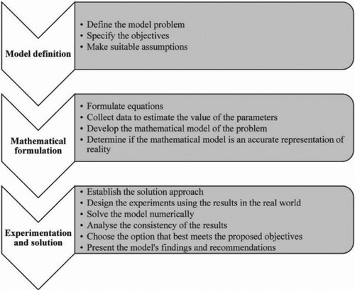
The key thought that lies behind this methodology is the problem definition, which explains the need for research based on a previous literature review. So the modelling objective is limited with the appropriate assumptions and necessary information to develop the model’s mathematical equations.- Here from the literature or via parameter estimation, the sets of values of the model’s input and output variables for SCP are defined. Then a suitable analytical or numerical method is selected to solve the developed mathematical model through equations. Finally, to examine the effects of the solution obtained in a case study of the footwear industry, the model is experimented with in several scenarios, and the consistency of the results obtained is analysed to support the findings and conclusions of this research.

4. Model definition

4.1. Problem description

Based on the conceptual model for LSCP 4.0 developed by Reyes, Mula, and Díaz-Madroñero (2023b), it is established that the problem under study is to determine the maximum profit in a traditional SC by employing lean, sustainable and resilient practices to cope with possible interruptions in the supply of raw materials and the flow of finished goods through correct LSCP. So the importance of minimising emissions, namely carbon dioxide (CO₂) (Fahimnia, Sarkis, and Eshragh 2015)_, and inventory waste (Oh and Jeong 2019) in SC planning is highlighted. Consequently, this research proposes an LSCP approach based on a new MILP model that places emphasis on JIT production which separately considers demand forecasts and firm customer orders for four SC levels. Hence the considered costs are classified as follows: production, inventory, backorder, transportation or supply of raw materials and finished goods, and carbon emissions from suppliers.

In resilience and sustainability terms, for the push system, and in order to manage demand variability, safety inventories proportional to the expected service level are incorporated (Brunaud et al. 2019), which is done with the flow of finished goods from warehouses to retailers that mitigate delays in the delivery of firm orders. However in the pull system, safety inventory is not considered because the essential success factor of JIT is stock minimisation (Z. Chen and Shang 2008). So a JIT model will provide a solution with zero safety inventory (Brunaud et al. 2019). The economic aspect also contemplates the maximisation of SC profits. For the environmental aspect, the selection of suppliers based on their CO₂ emissions is incorporated into the model (Das 2019; Fahimnia, Sarkis, and Eshragh 2015). Finally, the social sustainability aspect is addressed by, on the one hand, increasing service levels and, on the other hand, enhancing the incorporation of alternative SC suppliers to address local suppliers’ raw material supply problems (Shafiee, Zare Mehrjerdi, and Keshavarz 2021).

The main novelties of this study's proposal are manifested in three distinct areas related to LM, sustainability and resilience practices:

1. a mixed approach with two sources of push and pull demand in a traditional five-level SC context: second-level suppliers, first-level suppliers, manufacturers, warehouses or logistics operators and retailers. As such, demand management separately contemplates demand forecasts and firm orders from retailers at four levels. This is due to the fact that when taking the bullwhip effect as the variability of demand upstream at the SC levels (Fransoo and Wouters 2000), the further upstream one goes at the SC levels, the wider the variability of orders will be. This is aligned with F. Chen et al. (2000), who show that it is adequate to centralise demand information to reduce the magnitude of the bullwhip effect. For this reason, SC level five, which corresponds to second-level suppliers, has been designed with the aggregated demands (forecasts and firm order; see Figure 2). Additionally, to decrease variability in demand (Boutsioli 2010), an integrated inventory system for both sources of demand proposed by Rota, Thierry, and Bel (1997) is established, which takes into account firm orders and forecasts at the same time through the SC. This is specified as a combination of tactical and operational decisions based on forecasts and driven by firm order demand (Alavidoost, Jafarnejad, and Babazadeh 2021). Thus waste reduction in terms of waiting times and excess inventories is contemplated with the application of LM practices, such as JIT production, to meet the demand for firm orders at all levels where raw materials or finished goods are produced;

2. economic considerations for SC profit maximisation. This includes sales revenue from the push demand from forecasts and the pull demand from firm orders from retailers, which are analysed based on the conditions of each order and prioritised according to the profit they make;

3. a social approach to satisfying service levels in warehouse safety inventories is also included. Moreover, proactive measures for disruptive events (Llaguno, Mula, and Campuzano-Bolarin 2022) in the supply of raw materials are contemplated. Therefore, the selection of qualified first-level suppliers for the production of raw materials is based on their availability and ability to supply production plants. Finally, raw material supply problems are addressed by using alternative first-level suppliers.

Figure 2. LSCP 4.0 design.

A lean SC structure is presented with three-dimensional icons considering information flows of: raw materials at levels one and two for aggregate demand, finished goods at levels three to five for two types of demand.

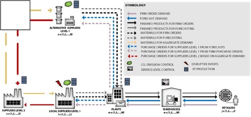
Figure 2 shows the flow of raw materials and finished goods of the SC under study, which has five levels: second-level suppliers, first-level suppliers, manufacturers, warehouses and retailers. Thus based on the LSCP 4.0 conceptual model of Reyes, Mula, and Díaz-Madroñero (2023b), the logistic flow of raw materials from different second-level suppliers to local and alternative first-level suppliers through several production plants is shown. Finally, finished goods are sent to warehouses to be delivered to retailers (see the model notation in Table 2).

Table 2. Notation of the LSCP 4.0 model.

Set of indexes
G	Set of second-level raw materials (indexed by g: g = 1, … ,$|G|$)
I	Set of finished goods (indexed by i: i = 1, … ,$|I|$)
J	Set of retailers of finished goods (indexed by j: j = 1, … ,$|J|$)
K	Set of first-level raw materials (indexed by k: k = 1, … ,$|K|$)
L	Set of first-level local suppliers (indexed by l: l = 1, … , $|L|$)
M	Set of production plants for finished goods (indexed by m: m = 1, … ,$|M|$)
N	Set of alternative first-level suppliers (indexed by n: n = 1, … ,$|N|$)
O	Set of firm orders for finished goods (indexed by o: o = 1, … ,$|O|$)
T	Set of time periods (indexed by t: t = 1, … ,$|T|$)
X	Set of second-level suppliers (indexed by x: x = 1, … ,$|X|$)
W	Set of warehouses for finished goods (indexed by w: w = 1, … ,$|W|$)
Data
${\beta }_{\mathrm{iw}}$	Level of risk of shortage of supply defined for i in w
$\rho a_{\mathrm{kl}}$	Cost of carbon emissions in production processes and logistics of supplier l to produce k
$\rho b_{\mathrm{kn}}$	Cost of carbon emissions in production processes and logistics of supplier n to produce k
$A{a}_{\mathrm{gk}}$	Required quantity of g to produce a unit of product k
$A{b}_{\mathrm{ki}}$	Required quantity of k to produce a unit of product i
$b{i}_{\mathrm{im}}$	Unit profit for producing i of firm orders in m
$\mathrm{Cc}{g}_{\mathrm{gx}}$	Penalty cost of a soft JIT production coverage constraint for material g on x
$\mathrm{Cc}{l}_{\mathrm{kl}}$	Penalty cost of a soft JIT production coverage constraint for material k on l
$\mathrm{Cc}{n}_{\mathrm{kn}}$	Penalty cost of a soft JIT production coverage constraint for material k on n
$\mathrm{Cc}{m}_{\mathrm{im}}$	Penalty cost of a soft JIT production coverage constraint for the product i on m
$C{f}_{\mathrm{km}}$	Backorder cost per unit of demand of k in m for the demand forecasts of finished goods
$\mathrm{Cf}{h}_{\mathrm{km}}$	Backorder cost per unit of demand of k in m for firm orders of finished goods
$\mathrm{Cf}{i}_{\mathrm{ij}}$	Backorder cost per unit of firm order demand of i in j
$\mathrm{Cf}{j}_{\mathrm{ij}}$	Backorder cost per unit of forecasting demand of i in j
$\mathrm{Cf}{l}_{\mathrm{gl}}$	Backorder cost per unit of first-level raw material demand g in l
$\mathrm{Cfl}{a}_{\mathrm{kl}}$	Backorder cost per unit of demand of k in l for demand forecasts of finished goods
$\mathrm{Cfl}{b}_{\mathrm{kl}}$	Backorder cost per unit of demand of k in l for firm orders of finished goods
$\mathrm{Cf}{n}_{\mathrm{gn}}$	Backorder cost per unit of first-level raw material demand g in n
$\mathrm{Cfn}{a}_{\mathrm{kl}}$	Backorder cost per unit of demand of k in n for demand forecasts of finished goods
$\mathrm{Cfn}{b}_{\mathrm{kl}}$	Backorder cost per unit of demand of k in n for firm orders of finished goods
$\mathrm{Cf}{w}_{\mathrm{iw}}$	Backorder cost per unit of forecasting demand for i in w
$\mathrm{Cf}{x}_{\mathrm{iw}}$	Backorder cost per unit of firm order demand for i in w
$\mathrm{Cf}{y}_{\mathrm{gx}}$	Backorder cost per unit of second-level raw material demand g in x
$C{j}_{\mathrm{ij}}$	Inventory storage unit cost i in j
$C{k}_{\mathrm{km}}$	Inventory storage unit cost of k in m
$\mathrm{Ck}{l}_{\mathrm{kl}}$	Inventory storage unit cost of k in l
$\mathrm{Ck}{n}_{\mathrm{kn}}$	Inventory storage unit cost of k in n
$C{l}_{\mathrm{klm}}$	Transport and distribution unit cost of k from l to m
$\mathrm{Cl}{x}_{\mathrm{gxl}}$	Transport and distribution unit cost of g from x to l for first-level raw material orders
$\mathrm{Cl}{y}_{\mathrm{gxn}}$	Transport and distribution unit cost of g from x to n for first-level raw material orders
$C{m}_{\mathrm{imw}}$	Transport and distribution unit cost of i from m to w
$C{n}_{\mathrm{knm}}$	Transport and distribution unit cost of k from n to m
$C{p}_{\mathrm{im}}$	Labour cost per hour for the regular time production of i in m
$\mathrm{Cp}{e}_{\mathrm{im}}$	Labour cost per hour for the overtime production of i in m
$\mathrm{Cp}{l}_{\mathrm{kl}}$	Labour cost per hour for the production of k in l
$\mathrm{Cp}{n}_{\mathrm{kn}}$	Labour cost per hour for the production of k in n
$\mathrm{Cp}{x}_{\mathrm{gx}}$	Labour cost per hour for the production of g in x for second-level raw material orders
$C{s}_{\mathrm{iwj}}$	Transport and distribution unit cost of i from w to j
$C{w}_{\mathrm{iw}}$	Inventory storage unit cost of i in w
$C{x}_{\mathrm{gx}}$	Inventory storage unit cost of the second-level raw material inventory of g in x
$\mathrm{Cx}{l}_{\mathrm{gl}}$	Inventory storage unit cost of the second-level raw material inventory of g in l
$\mathrm{Cx}{n}_{\mathrm{gn}}$	Inventory storage unit cost of the second-level raw material inventory of g in n
$D_{\mathrm{ijt}}$	Forecasted demand for i in j during time period t
$D{o}_{\mathrm{ijot}}$	Demand of product i in j to satisfy firm orders o during time period t
$E{C}_m$	Capacity hours for over time production of plant m
$F{l}_{\mathrm{kl}}$	Estimated carbon emissions generation of $\text{C}{\text{O}}_2$ as kg of first-level supplier l to produce k
$F{l}_{\mathrm{kn}}$	Estimated carbon emissions generation of $\text{C}{\text{O}}_2$ as kg of first-level supplier n to produce k
$E_{\mathrm{oimt}}$	Big number
$H{x}_{\mathrm{gx}}$	Programmed receptions of raw material g in x
$H{l}_{\mathrm{gl}}$	Programmed receptions of raw material g in l
$\mathrm{Hl}{a}_{\mathrm{kl}}$	Programmed receptions of raw material k in l for finished goods demand forecasts
$\mathrm{Hl}{b}_{\mathrm{okl}}$	Programmed receptions for firm orders o of finished goods of material k in l
$H{n}_{\mathrm{gn}}$	Programmed receptions of raw material g in n
$\mathrm{Hn}{a}_{\mathrm{kn}}$	Programmed receptions of raw material k in n for finished goods demand forecasts
$\mathrm{Hn}{b}_{\mathrm{okn}}$	Programmed receptions for firm orders o of finished goods of material k in n
$\mathrm{Hm}{a}_{\mathrm{km}}$	Programmed receptions of material k in m for finished goods demand forecasts
$\mathrm{Hm}{b}_{\mathrm{okm}}$	Programmed receptions for firm orders o of finished goods of material k in m
$\mathrm{Hm}{c}_{\mathrm{im}}$	Programmed receptions of the product i in m for finished goods demand forecasts
$\mathrm{Hm}{d}_{\mathrm{oim}}$	Programmed receptions for firm orders o of finished goods i in m
$\mathrm{Hw}{a}_{\mathrm{iw}}$	Programmed receptions of the product i in w for finished goods demand forecasts
$\mathrm{Hw}{b}_{\mathrm{oiw}}$	Programmed receptions for firm orders o of finished goods i in w
$\mathrm{Hj}{a}_{\mathrm{ij}}$	Programmed receptions of the product i in j for finished goods demand forecasts
$\mathrm{Hj}{b}_{\mathrm{oij}}$	Programmed receptions for firm orders o of finished goods i in j
$I{L}_l$	Inventory storage capacity of g in l
$\mathrm{IL}{A}_l$	Inventory storage capacity of k in l
$I{M}_m$	Inventory storage capacity of k in m
$\mathrm{IM}{A}_m$	Inventory storage capacity of i in m
$I{N}_n$	Inventory storage capacity of g in n
$\mathrm{IN}{A}_n$	Inventory storage capacity of k in n
$I{W}_w$	Inventory storage capacity of i in w
$I{X}_x$	Inventory storage capacity of g in x
$J{C}_j$	Inventory storage capacity of i in j
$L{C}_l$	Capacity hours for the regular-time production of first-level supplier l
$L{D}_n$	Capacity hours for the regular-time production of first-level supplier n
$L{X}_x$	Capacity hours for the regular-time production of second-level supplier x
$\mathrm{Lo}{l}_{\mathrm{klm}}$	Maximum transport capacity of k from l to m
$\mathrm{Lo}{n}_{\mathrm{knm}}$	Maximum transport capacity of k from n to m
$\mathrm{Lot}{g}_g$	Production lot size of raw material g
$\mathrm{Lot}{i}_i$	Production lot size of product i
$\mathrm{Lot}{k}_k$	Production lot size of raw material k
$\mathrm{LT}{j}_{\mathrm{iwj}}$	Lead time to deliver one unit of i from w to j
$\mathrm{LT}{l}_{\mathrm{klm}}$	Lead time to deliver one unit of k from l to m
$\mathrm{LT}{n}_{\mathrm{knm}}$	Lead time to deliver one unit of k from n to m
$\mathrm{LT}{x}_{\mathrm{gxl}}$	Lead time to deliver one unit of g from x to l
$\mathrm{LT}{y}_{\mathrm{gxn}}$	Lead time to deliver one unit of g from x to n
$N{C}_n$	Capacity hours for the regular-time production of supplier n
$P{C}_m$	Capacity hours for the regular-time production of plant m
$S{L}_{\mathrm{klm}}$	Available suppliers l that can supply materials k to m
$S{N}_{\mathrm{knm}}$	Available suppliers n that can supply materials k to m
$\mathrm{TS}{G}_{\mathrm{gx}}$	Required processing time (hours) to produce one unit of g in x
$\mathrm{TS}{L}_{\mathrm{kl}}$	Required processing time (hours) to produce one unit of k in l
$\mathrm{TS}{N}_{\mathrm{kn}}$	Required processing time (hours) to produce one unit of k in n
$T{S}_{\mathrm{im}}$	Required processing time (hours) to produce one unit of in m
$V{p}_{\mathrm{ij}}$	Price of product i agreed with retailer j
Decision variables
$b{a}_{\mathrm{oklmt}}$	1 if supplier l qualifies to ship at time k in t, 0 otherwise
$b{b}_{\mathrm{oknmt}}$	1 if supplier n qualifies to ship at time k in t, 0 otherwise
$g_{\mathrm{oimt}}$	Number of units to satisfy firm orders o of i produced at a regular time in m and t
$g{e}_{\mathrm{oimt}}$	Number of units to satisfy firm orders o of i produced overtime in m and t
$i{j}_{\mathrm{ijt}}$	Inventory quantity available of i in j to satisfy forecast demand and inventory to be used for the firm orders during t
$\mathrm{ij}{a}_{\mathrm{ijt}}$	Inventory quantity used to satisfy the forecast demand of i in j during t
$\mathrm{ij}{b}_{\mathrm{oijt}}$	Inventory quantity available to satisfy firm orders o of i in j during t
$\mathrm{ij}{c}_{\mathrm{oijt}}$	Inventory quantity used to satisfy firm orders o of i in j during t
$i{l}_{\mathrm{glt}}$	Inventory quantity of available g in l to satisfy the demand for the first-level raw materials during t
$\mathrm{il}{a}_{\mathrm{oklt}}$	Inventory quantity used to satisfy firm orders o of k in l during t
$\mathrm{il}{b}_{\mathrm{klt}}$	Inventory quantity available of k in l to satisfy the forecast demand and inventory to be used for the firm orders during t
$\mathrm{il}{c}_{\mathrm{oklt}}$	Inventory quantity available to satisfy firm orders o of k in l during t
$\mathrm{il}{d}_{\mathrm{klt}}$	Inventory quantity used to satisfy the forecast demand of k in l during t
$i{n}_{\mathrm{gnt}}$	Inventory quantity of available g in n to satisfy the demand for the first-level raw materials during t
$\mathrm{in}{a}_{\mathrm{oknt}}$	Inventory quantity used to satisfy firm orders o of k in n during t
$\mathrm{in}{b}_{\mathrm{knt}}$	Inventory quantity available of k in n to satisfy the forecast demand and inventory to be used for the firm orders during t
$\mathrm{in}{c}_{\mathrm{oknt}}$	Inventory quantity available to satisfy firm orders o of k in n during t
$\mathrm{in}{d}_{\mathrm{knt}}$	Inventory quantity used to satisfy the forecast demand of k in n during t
$i{m}_{\mathrm{kmt}}$	Inventory quantity available of k in m to satisfy the forecast demand and inventory to be used for the firm orders during t
$\mathrm{im}{a}_{\mathrm{kmt}}$	Inventory quantity used to satisfy the forecast demand of k in m during t
$\mathrm{im}{b}_{\mathrm{okmt}}$	Inventory quantity available to satisfy firm orders o of k in m during t
$\mathrm{im}{c}_{\mathrm{okmt}}$	Inventory quantity used to satisfy firm orders o of k in m during t
$i{p}_{\mathrm{imt}}$	Inventory quantity available of i in m to satisfy the forecast demand and inventory to be used for the firm orders during t
$\mathrm{ip}{a}_{\mathrm{imt}}$	Inventory quantity used to satisfy the forecast demand of i in m during t
$\mathrm{ip}{b}_{\mathrm{oimt}}$	Inventory quantity available to satisfy firm orders o of i in m during t
$\mathrm{ip}{c}_{\mathrm{oimt}}$	Inventory quantity used to satisfy firm orders o of i in m during t
$i{w}_{\mathrm{iwt}}$	Inventory quantity available of i in w to satisfy the forecast demand and inventory to be used for the firm orders during t
$\mathrm{iw}{a}_{\mathrm{iwt}}$	Inventory quantity used to satisfy the forecast demand of i in w during t
$\mathrm{iw}{b}_{\mathrm{oiwt}}$	Inventory quantity available to satisfy firm orders o of i in w during t
$\mathrm{iw}{c}_{\mathrm{oiwt}}$	Inventory quantity used to satisfy firm orders o of i in w during t
$i{x}_{\mathrm{gxt}}$	Inventory quantity of g in x to satisfy the demand for the second-level raw materials in t
$j{a}_{\mathrm{gxt}}$	Auxiliary variable to generate a soft production constraint for raw material g in x during t
$j{b}_{\mathrm{oklmt}}$	Auxiliary variable to generate a soft production constraint to satisfy firm orders o of k in l in m during t
$j{c}_{\mathrm{oknmt}}$	Auxiliary variable to generate a soft production constraint to satisfy firm orders o of k in n in m during t
$j{d}_{\mathrm{oimt}}$	Auxiliary variable to generate a soft production constraint to satisfy firm orders o of i in l in m during t
$l{g}_{\mathrm{gxt}}$	Number of lots to be produced of raw material g in x during t
$l{i}_{\mathrm{imt}}$	Number of lots to be produced of product i in m to satisfy the forecasted demand for the finished goods during t
$\mathrm{li}{a}_{\mathrm{oimt}}$	Number of lots to be produced of product i in m to satisfy firm orders o of the finished goods during t
$\mathrm{lk}{l}_{\mathrm{klmt}}$	Number of lots to be produced of raw material k in l to satisfy the forecasted demand for the finished goods in m during t
$\mathrm{lkl}{a}_{\mathrm{oklmt}}$	Number of lots to be produced of raw material k in l to satisfy firm orders o of the finished goods in m during t
$\mathrm{lk}{n}_{\mathrm{knmt}}$	Number of lots to be produced of raw material k in n to satisfy the forecasted demand for the finished goods in m during t
$\mathrm{lkn}{a}_{\mathrm{oknmt}}$	Number of lots to be produced of raw material k in n to satisfy firm orders o of the finished goods in m during t
$p{l}_{\mathrm{klmt}}$	Number of units k produced in l to satisfy the forecasted demand for the finished goods in m during t
$\mathrm{pl}{a}_{\mathrm{oklmt}}$	Number of k units produced in l to satisfy firm orders o of the finished goods in m during t
$p{n}_{\mathrm{knmt}}$	Number of k units produced in n to satisfy firm orders o of the finished goods in m during t
$\mathrm{pn}{a}_{\mathrm{oknmt}}$	Number of k units produced in n to satisfy firm orders o of the finished goods in m during t
$p_{\mathrm{imt}}$	Number of i units produced in m in a regular time to satisfy the forecast demand during t
$p{e}_{\mathrm{imt}}$	Number of i units produced in m in overtime to satisfy the forecast demand during t
$p{x}_{\mathrm{gxt}}$	Number of g units produced in x to satisfy the demand for the second-level raw materials during t
$q_{\mathrm{klmt}}$	Number of units of k supplied from l to m to satisfy the forecasted demand for the finished goods during t
$q{a}_{\mathrm{knmt}}$	Number of units of k supplied from n to m to satisfy the forecasted demand for the finished goods during t
$\mathrm{qb}{L}_{\mathrm{oklmt}}$	Number of units of k supplied to satisfy firm orders o from l to m during t
$\mathrm{qb}{N}_{\mathrm{oknmt}}$	Number of units of k supplied to satisfy firm orders o from n to m during t
$q{x}_{\mathrm{gxlt}}$	Number of units of g supplied from x to l to satisfy the demand for the first-level raw materials during t
$q{y}_{\mathrm{gxnt}}$	Number of units of g supplied from x to n to satisfy the demand for the first-level raw materials during t
$r{j}_{\mathrm{ijt}}$	Number of units of i in j required to satisfy the forecast demand during t
$\mathrm{rj}{a}_{\mathrm{oijt}}$	Number of units of i in j required to satisfy firm orders o during t
$r{l}_{\mathrm{glt}}$	Number of units of g in l required to satisfy the aggregate demand for the first-level raw materials during t
$\mathrm{rl}{a}_{\mathrm{klt}}$	Number of units of k in l required to satisfy the demand for the first-level raw materials during t
$\mathrm{rl}{b}_{\mathrm{oklt}}$	Number of units of k in l required to satisfy firm orders o during t
$r{m}_{\mathrm{kmt}}$	Number of units of k in m required to satisfy forecast demand t
$\mathrm{rm}{a}_{\mathrm{okmt}}$	Number of units of k in m required to satisfy firm orders o during t
$r{n}_{\mathrm{gnt}}$	Number of units of g in n required to satisfy the aggregate demand for the first-level raw materials during t
$\mathrm{rn}{a}_{\mathrm{knt}}$	Number of units of k in n required to satisfy forecast demand t
$\mathrm{rn}{b}_{\mathrm{oknt}}$	Number of units of k in n required to satisfy firm orders o during t
$r{p}_{\mathrm{imt}}$	Number of units of i in m required to satisfy forecast demand t
$\mathrm{rp}{a}_{\mathrm{oimt}}$	Number of units of i in m required to satisfy firm orders o during t
$r{w}_{\mathrm{iwt}}$	Number of units of i in w required to satisfy forecast demand t
$\mathrm{rw}{b}_{\mathrm{oiwt}}$	Number of units of i in w required to satisfy firm orders o during t
$r{y}_{\mathrm{gxt}}$	Number of units of g in x required to satisfy the demand for the second-level raw materials during t
$s{j}_{\mathrm{iwjt}}$	Number of units of i shipped from w to j to satisfy the forecast demand during t
$\mathrm{sj}{a}_{\mathrm{oiwjt}}$	Number of units of i shipped from w to j to satisfy firm orders o during t
$s{m}_{\mathrm{imwt}}$	Number of units of i shipped from m to w to satisfy the forecast demand during t
$\mathrm{sm}{a}_{\mathrm{oimwt}}$	Number of units of i shipped from m to w to satisfy firm orders o during t
$\mathrm{ss}{o}_{\mathrm{iw}}$	Quantity of the safety inventory of i in w to satisfy firm orders
$y_{\mathrm{oimt}}$	1 if the firm order o of i is produced in m during t, 0 otherwise

Firm orders and retailer forecasts can be viewed as two complementary types of external demands. This consequently generates two sources of demand for raw materials, which motivate the integration of resilient practices to cope with disruptive events from local first-level suppliers during disruptive events via the supply of raw materials from alternative suppliers. To pay more attention to sustainable practices, local first-level suppliers are prioritised based on lean and sustainability criteria. Firstly, each local supplier is rated based on its availability to supply raw materials; secondly, each local supplier is rated based on its availability to supply raw materials. Next when demand exceeds the local first-level suppliers’ supply capacity, part of production is allocated to qualified alternative suppliers to provide materials. To take into account the environmental aspect, the costs of direct $\text{C}{\text{O}}_2$ emissions from first-level suppliers’ production and logistics system are considered. Additionally, multitier production allows the sourcing of raw materials from second-level suppliers. This implies that finished goods manufacturers have limited production and storage capacity, and can operate on a regular or overtime basis. In addition, finished goods warehouses have limited storage capacity and are located at different distances from each production plant to supply retailers.

For a lean scheme, the SC in Figure 2 includes a JIT production system for firm order demand at all levels, which includes first- and second-level suppliers, and manufacturers that transport raw materials and finished goods to warehouses. One of the advantages of this system is the reduction in inventory costs. For this purpose, the proposed model allows the service level to be controlled through the simultaneous optimisation of safety inventory levels, which are calculated based on the quantities of finished goods supplied to distributors.

4.2. Assumptions

The parameters that characterise the different strategic decisions for supplying raw materials from second-level suppliers (selection of the local first-level suppliers), tactical (security inventories) and operational (manufacturing orders and shipments, among others) of LSCP are considered in the LSCP model, including the application of proactive resilience measures (alternative suppliers) to supply raw materials and the production of finished goods on a given planning horizon with t time periods. Finally, the proposed LSCP 4.0 model is based on the following key model inputs and assumptions:

• First- and second-level suppliers are considered to determine first- and second-tier requirements, deliveries and inventories in a synchronised manner, which can be beneficial for the SC (Coronado Mondragon and Lyons 2008)

• First-level suppliers’ supply capacity is finite and known. There is an ignorable risk of disruption for alternative suppliers. Therefore, the capacity of these alternative suppliers is considered infinite; i.e. they are always available to supply the necessary raw materials

• The production capacity of first-level suppliers is finite and known because most, if not all, production goes to the manufacturer

• The supply capacity of second-tier suppliers is not known because their production is not primarily for the manufacturer, and is considered to be unlimited

• There are regular and overtime production capacity constraints of finished goods manufacturers to minimise backorders

• Pre-established lot sizes are contemplated for producing raw materials and finished goods to satisfy manufacturing and logistics processes

• The variety of types of finished goods to be produced is known

• The number, location and capacity of production plants and warehouses are known

• The number and location of retailers are known

• Manufacturers and warehouses have storage capacity limitations due to space constraints

• Retailers’ finished goods demand forecasts are known, but irregular, because they present a variability coefficient over 0.2 (Winston 2004)

• The firm order demand for finished goods from retailers behaves like a JIT production system, which can also use the inventory generated from demand forecasts whenever necessary. A variability coefficient of firm order demand higher than 0.2 is also assumed (Winston 2004)

• The selling price of finished goods, the costs of raw materials, labour, storage, backorder and CO₂ emissions, are predetermined

• Production costs, which include standard production, and JIT production slack costs, inventory and transportation of raw materials and finished goods for demand from forecasts and firm orders, are considered to be the same

• The lead time of a finished good from warehouses to retailers is known during each planning time period

• To emulate JIT delivery for firm order demand, the local first-level suppliers who do not have supply availability are not assigned to produce raw materials. So alternative suppliers are assigned such orders. Disruptive events that affect lead time or capacity in the flow of raw materials from local suppliers may occur. In this case, alternative suppliers would also be assigned

• Due to the JIT delivery system, there is no lead time from manufacturing plants to finished goods warehouses

• JIT production is considered for first-level suppliers and firm order manufacturers. This is another LM aspect that MILP considers. Thus finished goods are produced as closely as possible to demand generation. For this purpose, pre-established penalty costs are considered for the possible need of slack for JIT production

• Manufacturing plants maintain raw materials inventories

• Finished goods warehouses maintain safety inventories only for the production that results from firm order demand, i.e. no safety inventories are considered for demand forecasts

• CO₂ emissions from first-level suppliers in production and logistics processes are known

5. Mathematical formulation

The MILP formulation of the LSCP 4.0 model uses the following mathematical notation (see Table 2).

The aim of the optimisation model in Equation (1) is to maximise the total profit as a measure of operational performance. Total profit, which considers the total incomes (TI) as defined in Equation (2), minus the total costs (TC) as defined in Equation (3), is a measure of overall economic sustainability. It is calculated based on the total revenues from the sale of finished goods warehouses to retailers to satisfy forecast demand and firm orders. A production profit is also considered for finished goods, which provides a production priority to satisfy firm orders. Costs are classified as follows: production planning costs (AC) from the suppliers and manufacturers detailed in Equation (4); inventory costs (IC) set out in Equation (5); cost of backorder demand (BC) defined in Equation (6); cost of the supply of raw materials and finished goods (MC) determined in Equation (7); cost of carbon emissions from the local and alternative first-level suppliers (LC) expressed in Equation (8); penalty costs (CC) for the need for slack to ensure that production is always as close as possible to the firm order demand requirement as a criterion for the JIT production expressed in Equation (9). (1) $\begin{array}{rl}\mathrm{Max}Z& =\mathrm{Total}\mathrm{Income}(\mathrm{TI})-\mathrm{Total}\mathrm{Costs}(\mathrm{TC})\end{array}$(1) (2) $\begin{array}{rl}\mathrm{TI}& =\sum _{\mathrm{iϵI}}\sum _{\mathrm{wϵW}}\sum _{\mathrm{jϵJ}}\sum _{\mathrm{tϵT}}V{p}_{\mathrm{ij}}s{j}_{\mathrm{iwjt}}\\ & +\sum _{\mathrm{oϵO}}\sum _{\mathrm{iϵI}}\sum _{\mathrm{wϵW}}\sum _{\mathrm{jϵJ}}\sum _{\mathrm{tϵT}}V{p}_{\mathrm{ij}}\mathrm{sj}{a}_{0\mathrm{iwjt}}\\ & +\sum _{\mathrm{oϵO}}\sum _{\mathrm{iϵI}}\sum _{\mathrm{mϵM}}\sum _{\mathrm{tϵT}}{b}_{\mathrm{im}}{y}_{\mathrm{oimt}}\end{array}$(2) (3) $\begin{array}{rl}\mathrm{TC}& =\mathrm{AC}+\mathrm{IC}+\mathrm{BC}+\mathrm{MC}+\mathrm{LC}+\mathrm{CC}\end{array}$(3) (4) $\begin{array}{rl}\mathrm{AC}& =\sum _{\mathrm{gϵG}}\sum _{\mathrm{xϵX}}\sum _{\mathrm{tϵT}}(\mathrm{Cp}{x}_{\mathrm{gx}}p{x}_{\mathrm{gxt}})\\ & +\sum _{\mathrm{kϵK}}\sum _{\mathrm{lϵL}}\sum _{\mathrm{mϵM}}\sum _{\mathrm{tϵT}}(\mathrm{Cp}{l}_{\mathrm{kl}}p{l}_{\mathrm{klmt}})\\ & +\sum _{\mathrm{oϵO}}\sum _{\mathrm{kϵK}}\sum _{\mathrm{lϵL}}\sum _{\mathrm{mϵM}}\sum _{\mathrm{tϵT}}(\mathrm{Cp}{l}_{\mathrm{kl}}\mathrm{pl}{a}_{\mathrm{oklmt}}b{a}_{\mathrm{oklmt}})\\ & +\sum _{\mathrm{kϵK}}\sum _{\mathrm{nϵN}}\sum _{\mathrm{mϵM}}\sum _{\mathrm{tϵT}}(\mathrm{Cp}{n}_{\mathrm{kn}}p{n}_{\mathrm{oknmt}})\\ & +\sum _{\mathrm{oϵO}}\sum _{\mathrm{kϵK}}\sum _{\mathrm{nϵN}}\sum _{\mathrm{mϵM}}\sum _{\mathrm{tϵT}}(\mathrm{Cp}{n}_{\mathrm{kn}}\mathrm{pn}{a}_{\mathrm{oknmt}}b{b}_{\mathrm{oknmt}})\\ & +\sum _{\mathrm{iϵI}}\sum _{\mathrm{mϵM}}\sum _{\mathrm{tϵT}}(C{p}_{\mathrm{im}}{p}_{\mathrm{imt}}+\mathrm{Cp}{e}_{\mathrm{im}}p{e}_{\mathrm{imt}})\\ & +\sum _{\mathrm{oϵO}}\sum _{\mathrm{iϵI}}\sum _{\mathrm{mϵM}}\sum _{\mathrm{tϵT}}(C{p}_{\mathrm{im}}{g}_{\mathrm{oimt}}+\mathrm{Cp}{e}_{\mathrm{im}}g{e}_{\mathrm{oimt}})\end{array}$(4) (5) $\begin{array}{rl}\mathrm{IC}& =\sum _{\mathrm{gϵG}}\sum _{\mathrm{xϵX}}\sum _{\mathrm{tϵT}}(C{x}_{\mathrm{gx}}i{x}_{\mathrm{gxt}})\\ & +\sum _{\mathrm{gϵG}}\sum _{\mathrm{lϵL}}\sum _{\mathrm{tϵT}}(\mathrm{Cx}{l}_{\mathrm{gl}}i{l}_{\mathrm{glt}})\\ & +\sum _{\mathrm{gϵG}}\sum _{\mathrm{nϵN}}\sum _{\mathrm{tϵT}}(\mathrm{Cx}{n}_{\mathrm{gn}}i{n}_{\mathrm{gnt}})\\ & +\sum _{\mathrm{kϵK}}\sum _{\mathrm{lϵL}}\sum _{\mathrm{tϵT}}(\mathrm{Ck}{l}_{\mathrm{kl}}\mathrm{il}{b}_{\mathrm{klt}})\\ & +\sum _{\mathrm{oϵO}}\sum _{\mathrm{kϵK}}\sum _{\mathrm{lϵL}}\sum _{\mathrm{tϵT}}(\mathrm{Ck}{l}_{\mathrm{kl}}\mathrm{il}{c}_{\mathrm{oklt}})\\ & +\sum _{\mathrm{kϵK}}\sum _{\mathrm{nϵN}}\sum _{\mathrm{tϵT}}(\mathrm{Ck}{n}_{\mathrm{kn}}\mathrm{in}{b}_{\mathrm{knt}})\\ & +\sum _{\mathrm{oϵO}}\sum _{\mathrm{kϵK}}\sum _{\mathrm{nϵN}}\sum _{\mathrm{tϵT}}(\mathrm{Ck}{n}_{\mathrm{kn}}\mathrm{in}{c}_{\mathrm{oknt}})\\ & +\sum _{\mathrm{kϵK}}\sum _{\mathrm{mϵM}}\sum _{\mathrm{tϵT}}(C{k}_{\mathrm{km}}i{m}_{\mathrm{kmt}})\\ & +\sum _{\mathrm{oϵO}}\sum _{\mathrm{kϵK}}\sum _{\mathrm{mϵM}}\sum _{\mathrm{tϵT}}(C{k}_{\mathrm{km}}\mathrm{im}{b}_{\mathrm{okmt}})\\ & +\sum _{\mathrm{iϵI}}\sum _{\mathrm{wϵW}}\sum _{\mathrm{tϵT}}(C{w}_{\mathrm{iw}}i{w}_{\mathrm{iwt}})\\ & +\sum _{\mathrm{oϵO}}\sum _{\mathrm{iϵI}}\sum _{\mathrm{wϵW}}\sum _{\mathrm{tϵT}}(C{w}_{\mathrm{iw}}\mathrm{iw}{b}_{\mathrm{oiwt}})\\ & +\sum _{\mathrm{iϵI}}\sum _{\mathrm{jϵJ}}\sum _{\mathrm{tϵT}}(C{j}_{\mathrm{ij}}i{j}_{\mathrm{ijt}})\\ & +\sum _{\mathrm{oϵO}}\sum _{\mathrm{iϵI}}\sum _{\mathrm{jϵJ}}\sum _{\mathrm{tϵT}}(C{j}_{\mathrm{ij}}\mathrm{ij}{b}_{\mathrm{oijt}})\end{array}$(5) (6) $\begin{array}{rl}\mathrm{BC}& =\sum _{\mathrm{gϵG}}\sum _{\mathrm{xϵX}}\sum _{\mathrm{tϵT}}(\mathrm{Cf}{y}_{\mathrm{gx}}r{y}_{\mathrm{gxt}})\\ & +\sum _{\mathrm{gϵG}}\sum _{\mathrm{lϵL}}\sum _{\mathrm{tϵT}}(\mathrm{Cf}{l}_{\mathrm{gl}}r{l}_{\mathrm{glt}})\\ & +\sum _{\mathrm{gϵG}}\sum _{\mathrm{nϵN}}\sum _{\mathrm{tϵT}}(\mathrm{Cf}{n}_{\mathrm{gn}}r{n}_{\mathrm{gnt}})\\ & +\sum _{\mathrm{kϵK}}\sum _{\mathrm{lϵL}}\sum _{\mathrm{tϵT}}(\mathrm{Cfl}{a}_{\mathrm{kl}}\mathrm{rl}{a}_{\mathrm{klt}})\\ & +\sum _{\mathrm{oϵO}}\sum _{\mathrm{kϵK}}\sum _{\mathrm{lϵL}}\sum _{\mathrm{tϵT}}(\mathrm{Cfl}{b}_{\mathrm{kl}}\mathrm{rl}{b}_{\mathrm{oklt}})\\ & +\sum _{\mathrm{kϵK}}\sum _{\mathrm{nϵN}}\sum _{\mathrm{tϵT}}(\mathrm{Cfn}{a}_{\mathrm{kn}}\mathrm{rn}{2}_{\mathrm{knt}})\\ & +\sum _{\mathrm{oϵO}}\sum _{\mathrm{kϵK}}\sum _{\mathrm{nϵN}}\sum _{\mathrm{tϵT}}(\mathrm{Cfn}{b}_{\mathrm{kn}}\mathrm{rn}{b}_{\mathrm{oknt}})\\ & +\sum _{\mathrm{kϵK}}\sum _{\mathrm{mϵM}}\sum _{\mathrm{tϵT}}(C{f}_{\mathrm{km}}r{m}_{\mathrm{kmt}})\\ & +\sum _{\mathrm{oϵO}}\sum _{\mathrm{kϵK}}\sum _{\mathrm{mϵM}}\sum _{\mathrm{tϵT}}(\mathrm{Cf}{h}_{\mathrm{km}}\mathrm{rm}{a}_{\mathrm{okmt}})\\ & +\sum _{\mathrm{iϵI}}\sum _{\mathrm{wϵW}}\sum _{\mathrm{tϵT}}(\mathrm{Cf}{w}_{\mathrm{iw}}r{w}_{\mathrm{iwt}})\\ & +\sum _{\mathrm{oϵO}}\sum _{\mathrm{iϵI}}\sum _{\mathrm{wϵW}}\sum _{\mathrm{tϵT}}(\mathrm{Cf}{x}_{\mathrm{iw}}\mathrm{rw}{a}_{\mathrm{oiwt}})\\ & +\sum _{\mathrm{iϵI}}\sum _{\mathrm{jϵJ}}\sum _{\mathrm{tϵT}}(\mathrm{Cf}{j}_{\mathrm{ij}}r{j}_{\mathrm{ijt}})\\ & +\sum _{\mathrm{oϵO}}\sum _{\mathrm{iϵI}}\sum _{\mathrm{jϵK}}\sum _{\mathrm{tϵT}}(\mathrm{Cf}{i}_{\mathrm{ij}}\mathrm{rj}{a}_{\mathrm{oijt}})\end{array}$(6) (7) $\begin{array}{rl}\mathrm{MC}& =\sum _{\mathrm{gϵG}}\sum _{\mathrm{xϵX}}\sum _{\mathrm{lϵL}}\sum _{\mathrm{tϵT}}(\mathrm{Cl}{x}_{\mathrm{gxl}}q{x}_{\mathrm{gxlt}})\\ & +\sum _{\mathrm{gϵG}}\sum _{\mathrm{xϵX}}\sum _{\mathrm{nϵN}}\sum _{\mathrm{tϵT}}(\mathrm{Cl}{y}_{\mathrm{gxn}}q{y}_{\mathrm{gxnt}})\\ & +\sum _{\mathrm{kϵK}}\sum _{\mathrm{lϵL}}\sum _{\mathrm{mϵM}}\sum _{\mathrm{tϵT}}(C{l}_{\mathrm{klm}}{q}_{\mathrm{klmt}})\\ & +\sum _{\mathrm{oϵO}}\sum _{\mathrm{kϵK}}\sum _{\mathrm{lϵL}}\sum _{\mathrm{mϵM}}\sum _{\mathrm{tϵT}}(C{l}_{\mathrm{klm}}\mathrm{qb}{L}_{\mathrm{oklmt}})\\ & +\sum _{\mathrm{kϵK}}\sum _{\mathrm{nϵN}}\sum _{\mathrm{mϵM}}\sum _{\mathrm{tϵT}}(C{n}_{\mathrm{knm}}q{a}_{\mathrm{knmt}})\\ & +\sum _{\mathrm{oϵO}}\sum _{\mathrm{kϵK}}\sum _{\mathrm{nϵN}}\sum _{\mathrm{mϵM}}\sum _{\mathrm{tϵT}}(C{n}_{\mathrm{klm}}\mathrm{qb}{N}_{\mathrm{oknmt}})\\ & +\sum _{\mathrm{iϵI}}\sum _{\mathrm{mϵM}}\sum _{\mathrm{wϵW}}\sum _{\mathrm{tϵT}}(C{m}_{\mathrm{imw}}s{m}_{\mathrm{imwt}})\\ & +\sum _{\mathrm{oϵO}}\sum _{\mathrm{iϵI}}\sum _{\mathrm{mϵM}}\sum _{\mathrm{wϵW}}\sum _{\mathrm{tϵT}}(C{m}_{\mathrm{imw}}\mathrm{sm}{a}_{\mathrm{oimwt}})\\ & +\sum _{\mathrm{iϵI}}\sum _{\mathrm{wϵW}}\sum _{\mathrm{jϵJ}}\sum _{\mathrm{tϵT}}(C{s}_{\mathrm{iwj}}s{j}_{\mathrm{iwjt}})\\ & +\sum _{\mathrm{oϵO}}\sum _{\mathrm{iϵI}}\sum _{\mathrm{wϵW}}\sum _{\mathrm{jϵJ}}\sum _{\mathrm{tϵT}}(C{s}_{\mathrm{iwj}}\mathrm{sj}{a}_{\mathrm{oiwjt}})\end{array}$(7) (8) $\begin{array}{rl}\mathrm{LC}& =\sum _{\mathrm{kϵK}}\sum _{\mathrm{lϵL}}\sum _{\mathrm{mϵM}}\sum _{\mathrm{tϵT}}\rho a_{\mathrm{kl}}F{l}_{\mathrm{kl}}(p{l}_{\mathrm{klmt}}+\mathrm{pl}{a}_{\mathrm{klmt}})\\ & +\sum _{\mathrm{kϵK}}\sum _{\mathrm{nϵN}}\sum _{\mathrm{mϵM}}\sum _{\mathrm{tϵT}}\rho b_{\mathrm{kn}}F{n}_{\mathrm{kn}}\\ & \times (p{n}_{\mathrm{knmt}}+\mathrm{pn}{a}_{\mathrm{knmt}})\end{array}$(8) (9) $\begin{array}{rl}\mathrm{CC}& =\sum _{\mathrm{gϵG}}\sum _{\mathrm{xϵX}}\sum _{\mathrm{tϵT}}(\mathrm{Cc}{g}_{\mathrm{gx}}j{a}_{\mathrm{gxt}})\\ & +\sum _{\mathrm{oϵO}}\sum _{\mathrm{kϵK}}\sum _{\mathrm{lϵL}}\sum _{\mathrm{mϵM}}\sum _{\mathrm{tϵT}}(\mathrm{Cc}{l}_{\mathrm{kl}}j{b}_{\mathrm{oklmt}})\\ & +\sum _{\mathrm{oϵO}}\sum _{\mathrm{kϵK}}\sum _{\mathrm{nϵN}}\sum _{\mathrm{mϵM}}\sum _{\mathrm{tϵT}}(\mathrm{Cc}{n}_{\mathrm{kn}}j{c}_{\mathrm{oknmt}})\\ & +\sum _{\mathrm{oϵO}}\sum _{\mathrm{iϵI}}\sum _{\mathrm{mϵM}}\sum _{\mathrm{tϵT}}(\mathrm{Cc}{m}_{\mathrm{im}}j{d}_{\mathrm{oimt}})\end{array}$(9)

The model is subject to the following constraints: (10) $\begin{array}{rl}& \mathrm{qb}{L}_{\mathrm{oklmt}}S{L}_{\mathrm{klm}}\le \mathrm{Lo}{l}_{\mathrm{oklt}}b{a}_{\mathrm{oklmt}}\mathrm{\forall o}\in O,k\in K,l\in L,\\ & m\in M,t>1\end{array}$(10) (11) $\begin{array}{rl}& \mathrm{qb}{N}_{\mathrm{oknmt}}S{N}_{\mathrm{knm}}\le \mathrm{Lo}{n}_{\mathrm{oknt}}b{b}_{\mathrm{oknmt}}\mathrm{\forall o}\in O,k\in K,\\ & n\in N,m\in M,t>1\end{array}$(11) (12) $\begin{array}{rl}& q_{\mathrm{klmt}-\mathrm{LTl}}+\sum _{\mathrm{oϵO}}\mathrm{qb}{L}_{\mathrm{oklmt}-\mathrm{LTl}}\le \mathrm{Lo}{l}_{\mathrm{klm}}\\ & \mathrm{\forall k}\in K,l\in L,m\in M,t>1\end{array}$(12) (13) $\begin{array}{rl}& q{a}_{\mathrm{knmt}-\mathrm{LTn}}+\sum _{\mathrm{oϵO}}\mathrm{qb}{N}_{\mathrm{oknmt}-\mathrm{LTn}}\le \mathrm{Lo}{n}_{\mathrm{knm}}\\ & \mathrm{\forall k}\in K,n\in N,m\in M,t>1\end{array}$(13) (14) $\begin{array}{rl}& \sum _{\mathrm{gϵG}}\mathrm{TS}{G}_{\mathrm{gx}}p{x}_{\mathrm{gxt}}\le L{X}_x\mathrm{\forall g}\in G,x\in X,t\in T\end{array}$(14) (15) $\begin{array}{rl}& \sum _{\mathrm{kϵK}}\mathrm{TS}{L}_{\mathrm{kl}}p{l}_{\mathrm{klmt}}+\sum _{\mathrm{oϵO}}\sum _{\mathrm{kϵK}}\mathrm{TS}{L}_{\mathrm{kl}}\mathrm{pl}{a}_{\mathrm{oklmt}}\le L{C}_l\\ & \mathrm{\forall o}\in O,l\in L,t\in T\end{array}$(15) (16) $\begin{array}{rl}& \sum _{\mathrm{kϵK}}\mathrm{TS}{N}_{\mathrm{kn}}p{n}_{\mathrm{knt}}+\sum _{\mathrm{oϵO}}\sum _{\mathrm{kϵK}}\mathrm{TS}{N}_{\mathrm{kn}}\mathrm{pn}{a}_{\mathrm{oknt}}\le N{C}_n\\ & \mathrm{\forall o}\in O,n\in N,t\in T\end{array}$(16) (17) $\begin{array}{rl}& \sum _{\mathrm{iϵI}}T{S}_{\mathrm{im}}{p}_{\mathrm{imt}}+\sum _{\mathrm{oϵO}}\sum _{\mathrm{iϵI}}T{S}_{\mathrm{im}}{g}_{\mathrm{oimt}}\le P{C}_m\\ & \mathrm{\forall m}\in M,t\in T\end{array}$(17) (18) $\begin{array}{rl}& \sum _{\mathrm{iϵI}}T{S}_{\mathrm{im}}p{e}_{\mathrm{imt}}+\sum _{\mathrm{oϵO}}\sum _{\mathrm{iϵI}}T{S}_{\mathrm{im}}g{e}_{\mathrm{oimt}}\le E{C}_m\\ & \mathrm{\forall m}\in M,t\in T\end{array}$(18) (19) $\begin{array}{rl}& p{x}_{\mathrm{gxt}}=L{g}_{\mathrm{gxt}}\ast \mathrm{Lot}{g}_g\mathrm{\forall g}\in G,x\in X,t\in T\end{array}$(19) (20) $\begin{array}{rl}& p{l}_{\mathrm{klmt}}=\mathrm{Lk}{l}_{\mathrm{klmt}}\ast \mathrm{Lot}{k}_k\\ & \mathrm{\forall k}\in K,l\in L,m\in M,t\in T\end{array}$(20) (21) $\begin{array}{rl}& \mathrm{pl}{a}_{\mathrm{oklmt}}=\mathrm{Lkl}{a}_{0\mathrm{klmt}}\ast \mathrm{Lot}{k}_k\\ & \mathrm{\forall o}\in O,\mathrm{\forall k}\in K,l\in L,m\in M,t\in T\end{array}$(21) (22) $\begin{array}{rl}& p{n}_{\mathrm{knmt}}=\mathrm{Lk}{n}_{\mathrm{knmt}}\ast \mathrm{Lot}{k}_k\\ & \mathrm{\forall k}\in K,n\in n,m\in M,t\in T\end{array}$(22) (23) $\begin{array}{rl}& \mathrm{pn}{a}_{\mathrm{oknmt}}=\mathrm{Lkn}{a}_{0\mathrm{knmt}}\ast \mathrm{Lot}{k}_k\\ & \mathrm{\forall o}\in O,\mathrm{\forall k}\in K,n\in N,m\in M,t\in T\end{array}$(23) (24) $\begin{array}{rl}& p_{\mathrm{imt}}=L{i}_{\mathrm{imt}}\ast \mathrm{Lot}{i}_i\mathrm{\forall i}\in i,m\in M,t\in T\end{array}$(24) (25) $\begin{array}{rl}& g_{\mathrm{oimt}}=\mathrm{Li}{a}_{\mathrm{oimt}}\ast \mathrm{Lot}{i}_i\\ & \mathrm{\forall o}\in O,\mathrm{\forall i}\in i,m\in M,t\in T\end{array}$(25) (26) $\begin{array}{rl}& p{x}_{\mathrm{gxt}}+j{a}_{\mathrm{gxt}}=\sum _{\mathrm{lϵL}}q{x}_{\mathrm{gxlt}}+\sum _{\mathrm{nϵN}}q{y}_{\mathrm{gxnt}}\\ & \mathrm{\forall g}\in G,x\in X,t\in T\end{array}$(26) (27) $\begin{array}{rl}& \mathrm{pl}{a}_{\mathrm{oklmt}}+j{b}_{\mathrm{oklmt}}=\sum _{\mathrm{mϵM}}\mathrm{qb}{L}_{\mathrm{oklmt}}\\ & \mathrm{\forall o}\in O,\mathrm{\forall k}\in K,l\in L,m\in M,t\in T\end{array}$(27) (28) $\begin{array}{rl}& \mathrm{pn}{a}_{\mathrm{oknmt}}+j{c}_{\mathrm{oknmt}}=\sum _{\mathrm{mϵM}}\mathrm{qb}{N}_{\mathrm{oknmt}}\\ & \mathrm{\forall o}\in O,\mathrm{\forall k}\in K,n\in N,m\in M,t\in T\end{array}$(28) (29) $\begin{array}{rl}& g_{\mathrm{oimt}}+j{d}_{\mathrm{oimt}}=\sum _{\mathrm{wϵW}}\mathrm{sm}{2}_{\mathrm{oimwt}}\\ & \mathrm{\forall o}\in O,\mathrm{\forall i}\in i,m\in M,t\in T\end{array}$(29) (30) $\begin{array}{rl}& p{x}_{\mathrm{gxt}}+i{x}_{\mathrm{gxt}-1}+H{x}_{\mathrm{gxt}}-r{x}_{\mathrm{gxt}-1}\\ & =\sum _{\mathrm{lϵL}}q{x}_{\mathrm{gxlt}}+\sum _{\mathrm{nϵN}}q{y}_{\mathrm{gxnt}}\mathrm{\forall g}\in G,x\in X,t\in T\\ & +i{x}_{\mathrm{gxt}}-r{x}_{\mathrm{gxt}}\end{array}$(30) (31) $\begin{array}{rl}& \sum _{\mathrm{xϵX}}q{x}_{\mathrm{gxlt}-\mathrm{LTx}}+i{l}_{\mathrm{glt}-1}+H{l}_{\mathrm{glt}}-i{l}_{\mathrm{glt}-1}\\ & =\sum _{\mathrm{kϵK}}A{a}_{\mathrm{gk}}(\sum _{\mathrm{mϵM}}p{l}_{\mathrm{klmt}}\mathrm{\forall g}\in G,l\in L,t\in T\\ & +\sum _{\mathrm{oϵO}}\sum _{\mathrm{mϵM}}\mathrm{pl}{a}_{\mathrm{oklmt}})+i{l}_{\mathrm{glt}}-r{l}_{\mathrm{glt}}\end{array}$(31) (32) $\begin{array}{rl}& \sum _{\mathrm{xϵX}}q{y}_{\mathrm{gxnt}-\mathrm{LTy}}+i{n}_{\mathrm{gnt}-1}+H{n}_{\mathrm{gnt}}-r{n}_{\mathrm{gnt}-1}\\ & \mathrm{\forall g}\in G,n\in N,t\in T\\ & =\sum _{\mathrm{kϵK}}A{a}_{\mathrm{gk}}\left(\sum _{\mathrm{mϵM}}p{n}_{\mathrm{knmt}}+\sum _{\mathrm{oϵO}}\sum _{\mathrm{mϵM}}\mathrm{pn}{a}_{\mathrm{oknmt}}\right)\\ & +i{n}_{\mathrm{gnt}}-r{n}_{\mathrm{gnt}}\end{array}$(32) (33) $\begin{array}{rl}& \sum _{\mathrm{mϵM}}p{l}_{\mathrm{klmt}-\mathrm{LTl}}+\mathrm{il}{b}_{\mathrm{klt}-1}+\mathrm{Hl}{a}_{\mathrm{klt}}-\sum _{\mathrm{oϵO}}\mathrm{il}{a}_{\mathrm{oklt}}\\ & -\mathrm{rl}{a}_{\mathrm{klt}-1}\mathrm{\forall k}\in K,l\in L,t\in T\\ & =\sum _{\mathrm{mϵM}}{q}_{\mathrm{klmt}}+\mathrm{il}{b}_{\mathrm{klt}}-\mathrm{rl}{a}_{\mathrm{klt}}\end{array}$(33) (34) $\begin{array}{rl}& \sum _{\mathrm{mϵM}}\mathrm{pl}{a}_{\mathrm{oklmt}-\mathrm{LTl}}\mathrm{ba}+\mathrm{il}{c}_{\mathrm{oklt}-1}+\mathrm{Hl}{b}_{\mathrm{oklt}}+\mathrm{il}{a}_{\mathrm{oklt}}\\ & -\mathrm{rl}{b}_{\mathrm{klt}-1}\mathrm{\forall o}\in O,\mathrm{\forall k}\in K,l\in L,t\in T\\ & =\sum _{\mathrm{mϵM}}\mathrm{qb}{L}_{\mathrm{oklmt}}+\mathrm{il}{c}_{\mathrm{oklt}}-\mathrm{rl}{b}_{\mathrm{oklt}}\end{array}$(34) (35) $\begin{array}{rl}& \sum _{\mathrm{mϵM}}p{n}_{\mathrm{knmt}-\mathrm{LTn}}+\mathrm{in}{b}_{\mathrm{knt}-1}+\mathrm{Hn}{a}_{\mathrm{knt}}\\ & -\sum _{\mathrm{oϵO}}\mathrm{in}{a}_{\mathrm{oknt}}-\mathrm{rn}{a}_{\mathrm{knt}-1}\mathrm{\forall k}\in K,n\in N,t\in T\\ & =\sum _{\mathrm{mϵM}}q{a}_{\mathrm{knmt}}+\mathrm{in}{b}_{\mathrm{knt}}-\mathrm{rn}{a}_{\mathrm{knt}}\end{array}$(35) (36) $\begin{array}{rl}& \sum _{\mathrm{mϵM}}\mathrm{pn}{a}_{\mathrm{oknmt}-\mathrm{LTn}}\mathrm{bb}+\mathrm{in}{c}_{\mathrm{oknt}-1}+\mathrm{in}{a}_{\mathrm{oknt}}+\mathrm{Hn}{b}_{\mathrm{oknt}}\\ & \mathrm{\forall o}\in O,\mathrm{\forall k}\in K,n\in N,t\in T-\mathrm{rn}{b}_{\mathrm{knt}-1}\\ & =\sum _{\mathrm{mϵM}}\mathrm{qb}{N}_{\mathrm{oknmt}}+\mathrm{in}{c}_{\mathrm{oknt}}-\mathrm{rn}{b}_{\mathrm{oknt}}\end{array}$(36) (37) $\begin{array}{rl}& \sum _{\mathrm{lϵL}}{q}_{\mathrm{klmt}}+\sum _{\mathrm{nϵN}}q{a}_{\mathrm{knmt}}+I{m}_{\mathrm{kmt}-1}+\mathrm{Hm}{a}_{\mathrm{kmt}}\\ & -\sum _{\mathrm{oϵO}}\mathrm{im}{c}_{\mathrm{okmt}}\mathrm{\forall k}\in K,m\in M,t\in T-R{m}_{\mathrm{kmt}-1}\\ & =\sum _{\mathrm{iϵI}}A{b}_{\mathrm{ki}}(p_{\mathrm{imt}}+p{e}_{\mathrm{imt}})+i{m}_{\mathrm{kmt}}-r{m}_{\mathrm{kmt}}\end{array}$(37) (38) $\begin{array}{rl}& \sum _{\mathrm{lϵL}}\mathrm{qb}{L}_{\mathrm{oklmt}}+\sum _{\mathrm{nϵN}}\mathrm{qb}{N}_{\mathrm{oknmt}}+\mathrm{Im}{b}_{\mathrm{okmt}-1}+\mathrm{Hm}{b}_{\mathrm{okmt}}\\ & +\mathrm{im}{c}_{\mathrm{okmt}}\mathrm{\forall o}\in O,k\in K,m\in M,\\ & t\in T-\mathrm{rm}{a}_{\mathrm{okmt}-1}\\ & =\sum _{\mathrm{iϵI}}A{b}_{\mathrm{ki}}(g_{\mathrm{oimt}}+g{e}_{\mathrm{oimt}})+\mathrm{im}{b}_{\mathrm{okmt}}\\ & -\mathrm{rm}{2}_{\mathrm{okmt}}\end{array}$(38) (39) $\begin{array}{rl}& p_{\mathrm{imt}}+p{e}_{\mathrm{imt}}+i{p}_{\mathrm{imt}-1}+\mathrm{Hm}{c}_{\mathrm{imt}}-\sum _{\mathrm{oϵO}}\mathrm{ip}{c}_{\mathrm{oimt}}\\ & -R{m}_{\mathrm{kmt}-1}\mathrm{\forall i}\in I,m\in M,t\in T-r{p}_{\mathrm{imt}-1}\\ & =\sum _{\mathrm{wϵW}}s{m}_{\mathrm{imwt}}+i{p}_{\mathrm{imt}}-r{p}_{\mathrm{imt}}\end{array}$(39) (40) $\begin{array}{rl}& g_{\mathrm{oimt}}+g{e}_{\mathrm{oimt}}+\mathrm{ip}{b}_{\mathrm{oimt}-1}+\mathrm{Hm}{d}_{\mathrm{oimt}}+\mathrm{ip}{c}_{\mathrm{oimt}}\\ & -\mathrm{rp}{a}_{\mathrm{oimt}-1}\mathrm{\forall o}\in O,i\in I,m\in M,t\in T\\ & =\sum _{\mathrm{wϵW}}\mathrm{sm}{a}_{\mathrm{oimwt}}+\mathrm{ip}{b}_{\mathrm{oimt}}-\mathrm{rp}{a}_{\mathrm{oimt}}\end{array}$(40) (41) $\begin{array}{rl}& \sum _{\mathrm{mϵM}}s{m}_{\mathrm{imwt}}+i{w}_{\mathrm{iwt}-1}+\mathrm{Hw}{a}_{\mathrm{iwt}}-\sum _{\mathrm{oϵO}}\mathrm{iw}{c}_{\mathrm{oiwt}}\\ & -r{w}_{\mathrm{iwt}-1}\mathrm{\forall i}\in I,w\in W,t\in T\\ & =\sum _{\mathrm{jϵJ}}s{j}_{\mathrm{iwjt}}+i{w}_{\mathrm{iwt}}-r{w}_{\mathrm{iwt}}\end{array}$(41) (42) $\begin{array}{rl}& \sum _{\mathrm{mϵM}}\mathrm{sm}{a}_{\mathrm{oimwt}}+\mathrm{iw}{b}_{\mathrm{oiwt}-1}+\mathrm{Hw}{b}_{\mathrm{oiwt}}+\mathrm{iw}{c}_{\mathrm{oiwt}}\\ & -\mathrm{rw}{a}_{\mathrm{oiwt}-1}\mathrm{\forall o}\in O,i\in I,w\in W,t\in T\\ & =\sum _{\mathrm{jϵJ}}\mathrm{sj}{a}_{\mathrm{oiwjt}}+\mathrm{iw}{b}_{\mathrm{oiwt}}-\mathrm{rw}{a}_{\mathrm{oiwt}}\end{array}$(42) (43) $\begin{array}{rl}& \sum _{\mathrm{wϵW}}s{j}_{\mathrm{iwjt}-\mathrm{LTj}}+i{j}_{\mathrm{ijt}-1}+\mathrm{Hj}{a}_{\mathrm{ijt}}-\sum _{\mathrm{oϵO}}\mathrm{ij}{c}_{\mathrm{oijt}}-r{j}_{\mathrm{ijt}-1}\\ & =D_{\mathrm{ijt}}\mathrm{\forall i}\in I,j\in J,t\in T+i{j}_{\mathrm{ijt}}-r{j}_{\mathrm{ijt}}\end{array}$(43) (44) $\begin{array}{rl}& \sum _{\mathrm{wϵW}}\mathrm{sj}{a}_{\mathrm{oiwjt}-\mathrm{LTj}}+\mathrm{ij}{b}_{\mathrm{oijt}-1}+\mathrm{Hj}{b}_{\mathrm{oijt}}+\mathrm{ij}{c}_{\mathrm{oijt}}\\ & -\mathrm{rj}{a}_{\mathrm{oijt}-1}\mathrm{\forall o}\in O,i\in I,w\in W,j\in J,\\ & =D{o}_{\mathrm{oijt}}+\mathrm{ij}{b}_{\mathrm{oijt}}-\mathrm{rj}{a}_{\mathrm{oijt}}t\in T\end{array}$(44) (45) $\begin{array}{rl}& \sum _{\mathrm{oϵO}}\mathrm{il}{a}_{\mathrm{oklt}}+\mathrm{il}{d}_{\mathrm{klt}}=\mathrm{il}{b}_{\mathrm{klt}}\mathrm{\forall k}\in K,l\in L,t\in T\end{array}$(45) (46) $\begin{array}{rl}& \sum _{\mathrm{oϵO}}\mathrm{in}{a}_{\mathrm{oknt}}+\mathrm{in}{d}_{\mathrm{knt}}=\mathrm{in}{b}_{\mathrm{knt}}\mathrm{\forall k}\in K,n\in N,t\in T\end{array}$(46) (47) $\begin{array}{rl}& \sum _{\mathrm{oϵO}}\mathrm{im}{c}_{\mathrm{okmt}}+\mathrm{im}{a}_{\mathrm{kmt}}=i{m}_{\mathrm{kmt}}\\ & \mathrm{\forall k}\in K,m\in M,t\in T\end{array}$(47) (48) $\begin{array}{rl}& \sum _{\mathrm{oϵO}}\mathrm{ip}{c}_{\mathrm{oimt}}+\mathrm{ip}{a}_{\mathrm{imt}}=i{p}_{\mathrm{imt}}\mathrm{\forall i}\in I,m\in M,t\in T\end{array}$(48) (49) $\begin{array}{rl}& \sum _{\mathrm{oϵO}}\mathrm{iw}{c}_{\mathrm{oiwt}}+\mathrm{iw}{a}_{\mathrm{iwt}}=i{w}_{\mathrm{iwt}}\mathrm{\forall i}\in I,w\in W,t\in T\end{array}$(49) (50) $\begin{array}{rl}& \sum _{\mathrm{oϵO}}\mathrm{ij}{c}_{\mathrm{oijt}}+\mathrm{ij}{a}_{\mathrm{ijt}}=i{j}_{\mathrm{ijt}}\mathrm{\forall i}\in I,j\in J,t\in T\end{array}$(50) (51) $\begin{array}{rl}& \mathrm{ss}{o}_{\mathrm{iw}}=\frac{\beta \sqrt{L_{\mathrm{iw}}}}{|T|}\sum _{\mathrm{oϵO}}\sum _{\mathrm{jϵJ}}\sum _{\mathrm{tϵT}}\mathrm{sj}{a}_{\mathrm{oiwjt}}\\ & \mathrm{\forall i}\in I,w\in W,j\in J,t\in T\end{array}$(51) (52) $\begin{array}{rl}& \sum _{\mathrm{oϵO}}\mathrm{iw}{o}_{\mathrm{oiwt}}\ge \mathrm{ss}{o}_{\mathrm{iw}}\mathrm{\forall i}\in I,w\in W,t\in T\end{array}$(52) (53) $\begin{array}{rl}& \sum _{\mathrm{gϵG}}i{x}_{\mathrm{gxt}}\le I{X}_x\mathrm{\forall x}\in X,t\in T\end{array}$(53) (54) $\begin{array}{rl}& \sum _{\mathrm{gϵG}}i{l}_{\mathrm{glt}}\le I{L}_l\mathrm{\forall l}\in L,t\in T\end{array}$(54) (55) $\begin{array}{rl}& \sum _{\mathrm{gϵG}}i{n}_{\mathrm{gnt}}\le I{N}_n\mathrm{\forall n}\in N,t\in T\end{array}$(55) (56) $\begin{array}{rl}& \sum _{\mathrm{kϵK}}\mathrm{il}{b}_{\mathrm{klt}}+\sum _{\mathrm{oϵO}}\sum _{\mathrm{kϵK}}\mathrm{il}{c}_{\mathrm{oklt}}\le \mathrm{IL}{A}_l\mathrm{\forall l}\in L,t\in T\end{array}$(56) (57) $\begin{array}{rl}& \sum _{\mathrm{kϵK}}\mathrm{in}{b}_{\mathrm{knt}}+\sum _{\mathrm{oϵO}}\sum _{\mathrm{kϵK}}\mathrm{in}{c}_{\mathrm{oknt}}\le \mathrm{IN}{A}_n\mathrm{\forall n}\in N,t\in T\end{array}$(57) (58) $\begin{array}{rl}& \sum _{\mathrm{kϵK}}i{m}_{\mathrm{kmt}}+\sum _{\mathrm{oϵO}}\sum _{\mathrm{kϵK}}\mathrm{im}{b}_{\mathrm{okmt}}\le I{M}_m\mathrm{\forall m}\in M,t\in T\end{array}$(58) (59) $\begin{array}{rl}& \sum _{\mathrm{iϵI}}i{p}_{\mathrm{kmt}}+\sum _{\mathrm{oϵO}}\sum _{\mathrm{iϵI}}\mathrm{ip}{b}_{\mathrm{oimt}}\le \mathrm{IM}{A}_m\\ & \mathrm{\forall m}\in M,t\in T\end{array}$(59) (60) $\begin{array}{rl}& \sum _{\mathrm{iϵI}}i{w}_{\mathrm{iwt}}+\sum _{\mathrm{oϵO}}\sum _{\mathrm{iϵI}}\mathrm{iw}{b}_{\mathrm{oiwt}}\le I{W}_w\mathrm{\forall w}\in W,t\in T\end{array}$(60) (61) $\begin{array}{rl}& \sum _{\mathrm{iϵI}}i{j}_{\mathrm{ijt}}+\sum _{\mathrm{oϵO}}\sum _{\mathrm{iϵI}}\mathrm{ij}{b}_{\mathrm{oijt}}\le J{C}_j\mathrm{\forall j}\in J,t\in T\end{array}$(61) (62) $\begin{array}{rl}& \sum _{\mathrm{wϵW}}\sum _{\mathrm{tϵT}}s{j}_{\mathrm{iwjt}}+\sum _{\mathrm{oϵO}}\sum _{\mathrm{wϵT}}\sum _{\mathrm{tϵT}}\mathrm{sj}{a}_{\mathrm{oiwjt}}\\ & \le \sum _{\mathrm{tϵT}}{D}_{\mathrm{ijt}}+\sum _{\mathrm{oϵT}}\sum _{\mathrm{tϵT}}D{o}_{\mathrm{oijt}}\mathrm{\forall i}\in I,j\in J\end{array}$(62) (63) $\begin{array}{rl}& g_{\mathrm{oimt}}\le E_{\mathrm{oimt}}{y}_{\mathrm{oimt}}\mathrm{\forall }o\in O,i\in I,m\in M,t\in T\end{array}$(63) (64) $\begin{array}{rl}& r{j}_{\mathrm{ijT}}=0\mathrm{\forall i}\in I,j\in J,T\end{array}$(64) (65) $\begin{array}{rl}& \mathrm{rj}{a}_{\mathrm{oijT}}=0\mathrm{\forall o}\in O,i\in I,j\in J,T\end{array}$(65) (66) $\begin{array}{rl}& g_{\mathrm{oimt}},g{e}_{\mathrm{oimt}},\mathrm{Hj}{a}_{\mathrm{ijt}},\mathrm{Hj}{b}_{\mathrm{oijt}},\mathrm{Hn}{a}_{\mathrm{knt}},H{l}_{\mathrm{glt}},\mathrm{Hl}{a}_{\mathrm{oklt}},\\ & \mathrm{Hm}{a}_{\mathrm{kmt}},\mathrm{\forall }\text{g}\in G,i\in I,j\in J,k\in K,\\ & \mathrm{Hm}{b}_{\mathrm{okmt}},\mathrm{Hm}{c}_{\mathrm{imt}},\mathrm{Hm}{d}_{\mathrm{oimt}},H{n}_{\mathrm{gnt}},\mathrm{Hn}{a}_{\mathrm{knt}},\mathrm{Hn}{b}_{\mathrm{oknt}},\\ & \mathrm{Hw}{a}_{\mathrm{iwt}},l\in L,m\in M,n\in N,o\in O,\\ & \mathrm{Hw}{b}_{\mathrm{oiwt}},H{x}_{\mathrm{gxt}},i{l}_{\mathrm{glt}},\mathrm{il}{a}_{\mathrm{oklt}},\mathrm{il}{b}_{\mathrm{klt}},\mathrm{il}{c}_{\mathrm{oklt}},\mathrm{il}{d}_{\mathrm{klt}},i{m}_{\mathrm{kmt}},\\ & \mathrm{im}{a}_{\mathrm{kmt}},w\in W,t\in T\\ & \mathrm{im}{b}_{\mathrm{okmt}},\mathrm{im}{c}_{\mathrm{okmt}},i{n}_{\mathrm{gnt}},\mathrm{in}{a}_{0\mathrm{knt}},\mathrm{in}{b}_{\mathrm{knt}},\mathrm{in}{c}_{\mathrm{oknt}},\mathrm{in}{d}_{\mathrm{knt}},\\ & i{p}_{\mathrm{imt}},\mathrm{ip}{b}_{\mathrm{oimt}},i{x}_{\mathrm{gxt}},j{a}_{\mathrm{gxt}},j{b}_{\mathrm{oklmt}},j{c}_{\mathrm{oknmt}},j{d}_{\mathrm{oimt}},l{g}_{\mathrm{gxt}},\\ & l{i}_{\mathrm{imt}},\mathrm{li}{b}_{\mathrm{oimt}},\mathrm{lk}{l}_{\mathrm{klmt}},\mathrm{lkl}{b}_{\mathrm{oklmt}},\mathrm{lk}{n}_{\mathrm{knmt}},\mathrm{lkn}{b}_{\mathrm{oknmt}},\mathrm{ss}{o}_{\mathrm{iw}},\\ & p_{\mathrm{imt}},p{e}_{\mathrm{imt}},p{l}_{\mathrm{klmt}},\mathrm{pl}{a}_{\mathrm{oklmt}},p{n}_{\mathrm{knmt}},\mathrm{pn}{a}_{\mathrm{oknmt}},p{x}_{\mathrm{gxt}},\\ & r{w}_{\mathrm{iwt}},q_{\mathrm{klmt}},q{a}_{\mathrm{knmt}},\mathrm{qb}{L}_{\mathrm{oklmt}},\mathrm{qb}{N}_{\mathrm{oknmt}},q{x}_{\mathrm{gxlt}},q{y}_{\mathrm{gxnt}},\\ & r{j}_{\mathrm{ijt}},\mathrm{rj}{a}_{\mathrm{oijt}},r{l}_{\mathrm{glt}},\mathrm{rl}{a}_{\mathrm{klt}},\mathrm{rl}{b}_{\mathrm{oklt}},r{m}_{\mathrm{kmt}},\mathrm{rm}{a}_{\mathrm{okmt}},r{n}_{\mathrm{gnt}},\\ & \mathrm{rn}{a}_{\mathrm{knt}},\mathrm{rn}{a}_{\mathrm{oknt}},r{p}_{\mathrm{imt}},\mathrm{rp}{a}_{\mathrm{oimt}},r{w}_{\mathrm{iwt}},\mathrm{rw}{a}_{\mathrm{oiwt}},r{y}_{\mathrm{gxt}},\\ & s{j}_{\mathrm{iwjt}},\mathrm{sj}{a}_{\mathrm{oiwjt}},s{m}_{\mathrm{imwt}},\mathrm{sm}{a}_{\mathrm{oimwt}},\mathrm{ss}{o}_{\mathrm{iw}}\ge 0\end{array}$(66) (67) $\begin{array}{rl}& g_{\mathrm{oimt}},g{e}_{\mathrm{oimt}},i{p}_{\mathrm{imt}},\mathrm{ip}{a}_{\mathrm{imt}},\mathrm{ip}{b}_{\mathrm{oimt}},\mathrm{ip}{c}_{\mathrm{oimt}},i{j}_{\mathrm{ijt}},\mathrm{ij}{a}_{\mathrm{ijt}},\\ & \mathrm{ij}{b}_{\mathrm{oijt}},\mathrm{\forall }\text{o}\in O,i\in I,j\in J,m\in M,\\ & \mathrm{ij}{c}_{\mathrm{oijt}},i{w}_{\mathrm{iwt}},\mathrm{iw}{a}_{\mathrm{iwt}},\mathrm{iw}{b}_{\mathrm{oiwt}},\mathrm{iw}{c}_{\mathrm{oiwt}},j{d}_{\mathrm{oimt}},p_{\mathrm{imt}},\\ & p{e}_{\mathrm{imt}},r{j}_{\mathrm{ijt}},w\in W,t\in T\\ & \mathrm{rj}{a}_{\mathrm{oijt}},r{p}_{\mathrm{imt}},\mathrm{rp}{a}_{\mathrm{oimt}},r{w}_{\mathrm{iwt}},\mathrm{rw}{a}_{\mathrm{oiwt}},s{j}_{\mathrm{iwjt}},\mathrm{sj}{a}_{\mathrm{oiwjt}},\\ & s{m}_{\mathrm{imwt}},\mathrm{sm}{a}_{\mathrm{oimwt}}ϵZ\end{array}$(67) (68) $\begin{array}{rl}& b{a}_{\mathrm{klt}}ϵ\{0,1\},b{b}_{\mathrm{knt}}ϵ\{0,1\},y_{\mathrm{oimt}}ϵ\{0,1\}\\ & \mathrm{\forall i}\in I,k\in K,l\in L,m\in M,n\in N,o\in O,t\in T\end{array}$(68)

Equations (10) and (11) represent the local and alternative first-level suppliers that qualify in time (Tirkolaee et al. 2020) for the supply of raw materials to fulfil firm order demand. Equations (12) and (13) ensure that shipments of the materials for forecast demands and firm orders do not exceed the supply capacity during each planning period from each local and alternative first-level supplier to all the production plants (Farahani and Elahipanah 2008). Unlike conventional SCP models, in this research five-level SC constraints are developed for the first time for two types of finished goods demand: the first one from demand forecasts and the second one for firm orders. Equations (14)–(16) limit the capacity for the raw materials production by the first- and second-level suppliers. Equations (17) and (18) limit the capacity for the finished goods production in regular working hours and overtime, respectively. Equations (19)–(25) allow the total production of the first-level and second-level materials, as well as finished goods, during each period of time to be multiples of a given lot that may be required for the needs of each production process. This group of lot-size constraints is deactivated at the different SC levels when they are not required.

Equations (26)–(29) correspond to the JIT production of raw materials and finished goods. This contemplates a penalty cost in the objective function due to the need for slack to cover parts production. Here the function of penalty costs is to ensure that the parts production levels at the end of each time period come as close as possible to the sum of the demands during the following time periods according to the supply cover. This group of lean constraints is activated at the different SC levels when the model is pull and deactivated in the push model.

With raw materials, Equations (30)–(32) represent the inventory balances of the second-level suppliers, where the requirements to produce first-level raw materials are entered. In Equations (33)–(38), the inventory balances of the first-level suppliers are detailed, where inputs correspond to the quantities of raw materials to be ordered, and come from the finished goods production needs of each planning period. Equations (34) and (36) present a product of a binary decision variable and a continuous decision variable, which result in an MINLP model. To avoid such non linearity, this variable relation can be converted into a linear expression by adding an auxiliary variable according to (Williams 2013). Equations (39) and (40) consider the inventory balances of finished goods manufacturers. Equations (41) and (42) establish the inventory balances of warehouses for finished goods demand forecasts and firm orders, respectively. Equations (43) and (44) determine retailers’ inventory balances, where inputs correspond to shipped quantities, the backorder of firm orders, the quantities required to meet demand forecasts and the inventory during the previous period. Outputs refer to the demand forecasts and firm orders for each finished good. Here the delivery time from warehouses to distributors is considered. It should be noted that Constraints (33) through to (44) integrate inventories from both demand sources, i.e. forecasts and firm orders. Equations (45) through to (50) ensure that the total amount of inventory does not exceed the inventory level capacity levels at the first-level suppliers, manufacturers, warehouses and distributors.

Regarding the safety inventory in finished goods warehouses for the firm orders of the push model, and considering that the service level is given, the lead time ($L_{\mathrm{iw}}$) is constant and the standard deviation is proportional to the flow of finished goods that must cover variation in demand. Thus the safety inventory is proportional to the production flow proposed by (Brunaud et al. 2019). Parameter β indicates the level of risk of stockouts defined as a percentage and T is the final planning period. In this case, the safety inventory would be a percentage of the quantity supplied from warehouses to retailers multiplied by the square root of the replenishment lead time. In previous works, the safety inventory was not a variable, but a given parameter. Equation (51) provides a method to optimise the safety inventory according to the flow to the retailer. In the proposed formulation, safety inventory is used as the lower inventory limit (51) and the upper inventory level is limited by Equation (52). These two equations are deactivated at warehouse levels when they are not required.

Equations (53) through to (55) limit the storage capacity of the second-level raw materials by suppliers. Equations (56) through to (58) set limits on the storage of the first-level raw materials at the local, alternative suppliers and finished goods manufacturers. Consequently, Equations (59), (60) and (61) ensure that the inventory for both firm orders and forecasts does not exceed the storage capacity at manufacturers, warehouses and retailers, respectively. Equation (62) ensures that the finished goods supplied from warehouses to distributors do not exceed demand. Equation (63) guarantees production prioritisation for the demand from firm orders in relation to the demand from forecasts. This generates a fixed extra profit charge when a firm order is produced, which is discounted from TI at the end of the model run to obtain the real total profit. Equation (64) ensures that the forecast demand of the production plan will be satisfied during the last planning period T. This is a pull criterion because it allows a delay in the demand for firm orders so that this production will be planned whenever required. Equation (65) ensures that the firm orders of the production plan will be satisfied during the last time period T. These two last constraints are activated or deactivated according to production system requirements.

Equation (66) establishes the non-negativity condition for the decision variables. Equation (67) refers to the integer condition for the decision variables. Finally, the formulations in Equation (68) establish the condition of the binary variables.

6. Experimentation and solution

6.1. Solution approach

The established solution approach is the exact resolution of the MILP model through the CPLEX solver. So the LSCP4.0 model was implemented in modelling language MPL (mathematical programming language). Finally, the model’s input and output data are managed with a relational database. The multilevel MILP was solved on a computer with 12 Gb RAM and an Intel® Core® i7-1065G7 microprocessor [email protected] GHz frequency.

In addition, the input data are provided in the form of a normalised metastructure (see appendices) for LSCP 4.0 cloud computing to be integrated into the C2NET manufacturing platform (Andres, Poler, and Sanchis 2021; Reyes et al. 2024).

6.2. Real-world case study

The case company (BUF) is engaged in the manufacture and distribution of leather and thermoplastic safety footwear, among others. The company traditionally follows a serial production strategy for manufacturing safety footwear based on forecast demand. However, customers constantly diversify their orders in terms of quantity and variety of models. This has led decision makers to plan demand for firm orders with production prioritisation from a lean perspective for waste reduction, which forces suppliers to respond more quickly. With the COVID-19 pandemic however, severe fluctuations in demand, disruptions in SC structures, and changes in delivery times from suppliers, took place. BUF has two production plants (M = 2) and a central warehouse (W = 1) that consolidate all the finished goods to be shipped to a variety of retailers, namely the six main retailers (J = 6), to which the three main footwear models (I = 3) are delivered from two sources of demand: (a) forecasted push demand; (b) pull demand from firm orders (O = 16). BUF imports or produces directly most of its raw materials. However, on the bill of materials (BOM) for footwear manufacturing there is a group of eight essential raw materials (K = 8) that are supplied by several local first-level suppliers (L = 5), as well as a group of alternative suppliers (N = 4) that can supply these materials if needed. Of these materials, two of them, given their importance (leather and soles), are exploded on a second BOM to be supplied by second-level suppliers (X = 4), for which 15 raw materials are produced (G = 15). For the planning horizon, a 16-week tactical and operational decision level (T = 16) is considered. In inventory management terms, BUF and all the first- and second-level material suppliers have established policies, such as limited storage capacity, scheduled receipts and a predefined supply time. The harmful emissions measured as kilograms of CO₂ from manufacturing footwear raw materials at the local and alternative first-level suppliers are based on the results of (Cheah et al. 2013). Additionally, production capacity, which is lot-based, is limited at all the levels, and overtime can be worked only in BUF's production plants.

The other features that lead to different size problems in BUF are described in Table 3. The small-sized problem comprises demand forecasts and minimum firm orders to obtain a solution. The medium-sized problem specifies the actual values of both demand sources. The large-sized problem details a scenario with such demand increases that the production system is brought to its maximum capacity. So to perform experiments, 21 scenarios were designed at each SC level for every problem type, which consider applying MRP criteria for a push system and JIT production for a pull system (see Table 3).

Table 3. Design of the experiments for each SC level.

Scenario code	Production strategy (MRP/JIT)	Backorders	Suppliers level 2 (x)	Local suppliers level 1 (l)	Alternative suppliers level 1 (n)	Plants (m)	Warehouses (w)	Retailers (j)
e1	MRP	+	X	X	X	X	SS	X
e2	MIXED	+	X	X	X	O	SS	X
e3	MIXED	+	O	X	X	X	SS	X
e4	MIXED	+	X	O	O	O	SS	X
e5	MIXED	+	X	O	O	X	SS	X
e6	JIT	+	O	O	O	O		X
e7	MIXED	+	X	X	X	O		X
e8	MIXED	+	O	X	X	X		X
e9	MIXED	+	X	O	O	X		X
e10	MIXED	+	O	O	O	X		X
e11	JIT	+	O	O	O	O	SS	X
e12	MRP ϟ	+	X	X	X	X	SS	X
e13	BEST MIXED ϟ	+	X	X	X	O		X
e14	MRP *	+	X	X	X	X	SS	X
e15	JIT *	+	O	O	O	O		X
e16	MRP	†	X	X	X	X	SS	X
e17	JIT	†	O	O	O	O		X
e18	BEST MIXED	†	X	X	X	O	SS	X
e19	MRP	++	X	X	X	X	SS	X
e20	JIT	++	O	O	O	O		X
e21	BEST MIXED	++	X	X	X	O	SS	X

Note: O: pull system with JIT production; X: push system with MRP tools; SS: safety inventory; +: null backorders during the last time period for demand forecasts; †: null backorders during the last time period for firm orders; ++: null backorders during the last time period for forecasts and firm orders; ϟ: all the demand consolidated for firm orders; *without lot-sizing production; BLANK: with no safety inventory.

Table 4 shows the optimality gap value, runtime, costs, revenues and final profit in each scenario for the three tested size problems. Here in a demand variability context, mixed strategy e7 generates the lowest inventory and backorder costs, which provides the highest economic profit. There is, however, a cost improvement from changes in the production plan when consolidating demand from forecasts into demand from firm orders (see scenario e13). It is also worth noting that when fully MRP and JIT scenarios are experimented (e1 and e6), but without production lot sizes (e14 and e15), there is improvement in profits. Thus, the fact that the results obtained from the best scenarios are the same for the three tested size problems is confirmed. However, when experimenting with the scenarios with the highest economic profit (e1, e6 and e7) of medium- and large-sized problems in the scenarios with null backorders during the last time period for firm orders (e16, e17 and e18), an improvement in e1 is noticed (MRP strategy), which is depicted in e16. Thus MRP scenarios perform better with lot sizing and null backorders for demand forecasts during the last time period constraints. Moreover for the small-sized problem, e17 improves performance on e6 (JIT strategy). Hence JIT scenarios perform better without lot-sizing constraints and with null backorders for firm orders during the last time period. Regarding the MRP and BEST MIXED strategies, scenarios e19 and e2 with null backorders constraints during the last time period for forecasts and firm orders improve profits in large-sized problems by producing more and diminishing backorders along the time horizon. Finally for the JIT scenarios with null backorders constraints for demand forecasts and firm orders during the last time period for large-sized problems, no solution is obtained with the current computation resources. Thus it can be stated that JIT scenarios are computationally more costly than MRP and MIXED ones.

Table 4. Objective function values and runtime per instance.

				Total costs (TC) ($)						Total incomes (TI) ($)
Size problems	Scenario code	Gap (%)	Runtime (seconds)	Production (AC)	Penalisation of JIT production coverage (CC)	Inventory (IC)	Transport (MC)	Backorder (BC)	CO2 emissions (LC)	Sales	Fixed charge for production of firm orders	Total profit ($)
Small	e1	0.02	696	93740	0	2061	16294	0	1980	160.495	92160	46420
	e2	0.02	1140	93744	0	2054	16294	0	1979	160.495	92160	46424
	e3	0.61	1265	93856	0	9495	16209	548	1979	160.495	92160	38408
	e4	3.57	32400	94285	620	6411	16361	10	2076	160.495	92160	40732
	e5	3.70	32400	94266	540	6239	16465	182	2067	160.447	92160	40688
	e6	4.46	32400	94208	685	13852	16154	184	2120	160.495	92160	33292
	e7	0.00	723	93617	0	1956	16279	0	1977	160.495	92160	46666
	e8	4.54	5160	94208	685	13852	16154	184	2120	160.495	92160	33292
	e9	5.02	32400	94468	380	6932	16445	119	2528	160.495	92160	39623
	e10	4.77	32400	94346	300	14029	16258	64	2182	160.495	92160	33316
	e11	4.10	32400	94307	765	13761	16221	0	2087	160.495	92160	33354
	e12	0.34	472	119211	0	3708	21051	936	4922	201.760	92160	51932
	e13	0.25	2275	118816	0	3444	21006	961	4804	201.760	92160	52729
	e14	0.00	725	93618	0	1952	16279	0	1977	160.495	92160	46669
	e15	3.7	32400	94227	690	12169	16506	279	2139	160.495	92160	34485
	e16	0.10	871	93739	0	2061	16294	101	1980	160.495	92160	46320
	e17	4.01	21780	94283	155	13922	16305	17	2070	160.495	92160	33743
	e18	0.03	935	93712	0	2062	16289	0	1979	160.452	92160	46410
	e19	0.06	234	93735	0	2062	16293	55	1979	160.495	92160	46371
	e20	4.37	21840	94311	375	14013	16243	36	2146	160.495	92160	33371
	e21	0.02	167	93738	0	2061	16293	0	1979	160.495	92160	46424
Medium	e1	0.19	671	302.676	0	7597	49818	581	8.679	481.430	92160	112079
	e2	0.21	244	302.489	0	7.644	49.788	793	8.706	481.430	92160	112010
	e3	0.01	1748	302538	0	15017	49688	340	8678	481.430	92160	105169
	e4	3.46	32400	303712	385	11990	50039	844	9041	481.430	92160	105419
	e5	3.20	32400	303853	305	11744	50000	782	8947	481.430	92160	105799
	e6	3.77	32400	303496	191	19583	49865	751	9091	481.430	92160	98453
	e7	0.00	151	302403	0	7165	49767	410	8636	481.430	92160	113049
	e8	0.00	90	302481	0	14474	49661	370	8667	481.430	92160	105777
	e9	4.94	32400	305733	310	12126	50404	442	9252	481.430	92160	103163
	e10	4.39	32400	304746	610	18609	49795	806	9552	481.430	92160	97312
	e11	3.57	32400	303899	390	19226	50044	822	8773	481.430	92160	98276
	e12	0.47	4740	311330	0	8750	51108	1522	8798	493.312	92160	111804
	e13	0.16	1250	310677	0	7449	50950	1582	8610	493.312	92160	114044
	e14	0.02	568	302556	0	7633	49798	360	8656	481.430	92160	112427
	e15	5.28	32400	304654	610	19872	50064	681	9881	481.430	92160	95668
	e16	0.10	195	302561	0	7618	49799	335	8681	481.430	92160	112436
	e17	4.17	32400	304647	80	18796	50086	494	9474	481.430	92160	97853
	e18	0.03	846	302484	0	7640	49788	373	8704	481.430	92160	112441
	e19	0.07	1088	302484	0	7640	49788	373	8704	481.430	92160	112321
	e20	4.51	19688	302563	0	7609	49799	460	8678	481.430	92160	96976
	e21	0.00	144	305261	305	19551	49983	130	9224	481.430	92160	112440
Large	e1	0.1	1292	980904	0	20916	150777	23270	30758	1.442.490	92160	235865
	e2	0.11	794	980963	0	20925	150784	23416	30766	1.442.498	92160	235644
	e3	0.01	317	981484	0	28313	150779	23133	30761	1.442.498	92160	228028
	e4	9.20	32400	987498	590	34500	151525	26172	35457	1.443.698	92160	207956
	e5	11.42	32400	991616	666	37917	151612	26042	34357	1.444.290	92160	202080
	e6	5.36	32400	984795	525	37750	151174	27715	32980	1.444.290	92160	209351
	e7	0.01	72	978634	0	20148	150548	23127	30814	1.442.498	92160	239227
	e8	0.00	65	979175	0	27568	150546	23086	30813	1.442.498	92160	231310
	e9	5.55	32400	984394	305	28623	150998	23213	33956	1.442.498	92160	221009
	e10	11.35	32400	996732	460	35572	151706	26340	35402	1.444.290	92160	198078
	e11	6.49	32400	988841	560	36522	151397	24384	34188	1.444.130	92160	208238
	e12	0.04	480	980904	0	20916	150777	23270	30758	1.442.490	92160	235865
	e13	0.01	62	978634	0	20148	150548	23127	30814	1.442.498	92160	239227
	e14	0.00	1826	980913	0	20932	150780	23580	30762	1.442.498	92160	235531
	e15	7.88	32400	984673	454	42738	151699	23744	33794	1.444.290	92160	207188
	e16	0.19	997	999563	0	22540	153067	15123	30358	1.460.616	92160	239965
	e17	N/A	N/A	N/A	N/A	N/A	N/A	N/A	N/A	N/A	N/A	N/A
	e18	0.13	1560	999530	0	22550	153065	14939	30360	1.460.648	92160	240204
	e19	0.11	1183	999580	0	22602	153073	14855	30366	1.460.734	92160	240258
	e20	N/A	N/A	N/A	N/A	N/A	N/A	N/A	N/A	N/A	N/A	N/A
	e21	0.08	1516	999493	0	22619	153059	14787	30347	1.460.648	92160	240343

Note: Total profit = Sales – Total costs (TC); N/A: non-feasible solution.

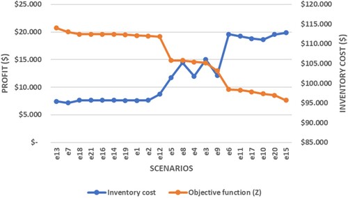
By considering the cost with the highest standard deviation in the scenarios under study, Figure 3 provides the results of the experiments in inventory cost and total profit terms for the medium-sized problem. The total profit results are grouped in descending order across the studied scenarios. This analysis shows that the BEST MIXED scenarios (e13, e7, e18 and e21), which provide the highest overall profits are the mixed scenarios, which have lower inventory costs. Thus our results support the approach of (Ganeshan 1999), which states that a mixed push–pull system generates better profits due to lower costs.

Figure 3. Relation between inventory cost and profits for the medium-sized problem.

A relation between inventory costs and total model profits is presented for each scenario of the performed experiments for the medium-sized problem.

In terms of the solver's solution optimisation, Table 5 illustrates the computational efficiency related to the three main scenarios of the proposed SC planning model: (a) MRP; (b) JIT; (c) the best MIXED. The computational efficiency for each model at the three tested size problems is also included. The data are related to the iterations that the solver uses to find the solution, number of constants, variables, integers, non-zero elements and the density of the constraint set to execute the model. These iteration values are the same for the medium and large sizes, which implies that the model needs more time to obtain an optimal solution due to the large amounts of data. So a time limit of 9 h is set in each run.

Table 5. Computational efficiency.

Size problems	Scenario code	Iterations	Constraints	Variables	Integers	Non-zeros	Density (%)
Small	e1	88317	238670	354192	71760	950706	11.00
	e6	5408987	276494	354192	71760	1108722	11.00
	e7	35299	237185	354195	71760	951525	11.00
Medium	e1	131338	237185	354195	71760	951525	11.00
	e6	6120129	276494	354192	71760	1108722	11.00
	e7	36270	238670	354192	71760	950706	11.00
Large	e1	98724	237185	354195	71760	951525	11.00
	e6	8981257	276494	354192	71760	1108722	11.00
	e7	38050	238670	354192	71760	950706	11.00

It is important to highlight the analysis of the bullwhip effect measure (BEM) according to the method proposed by Fransoo and Wouters (2000). In line with this, the BEM calculation is determined for the products and orders aggregated in the set of SC levels as the quotient of the coefficient of variation of demand generated by this set of levels $(C_{\mathrm{out}})$ and the coefficient of variation of demand received by this level $(C_{\mathrm{in}})$, using the expressions presented in Equations (69)–(71). Here the $C_{\mathrm{out}}$ calculation is made with the standard deviation (σ) of the demand going out to the next upstream level $D_{\mathrm{out}}$, and with the average (μ) of such demand during the time interval (t,t + T). In addition, $C_{\mathrm{in}}$ is calculated in a similar way, but with demand coming from the next downstream level. (69) $\begin{array}{rl}\text{BEM}& =\frac{C_{\mathrm{out}}}{C_{\mathrm{in}}}\end{array}$(69) (70) $\begin{array}{rl}{C}_{\mathrm{out}}& =\frac{\sigma (D_{\mathrm{out}}(t,t+T))}{\mu (D_{\mathrm{out}}(t,t+T))}\end{array}$(70) (71) $\begin{array}{rl}{C}_{\mathrm{in}}& =\frac{\sigma (D_{\mathrm{in}}(t,t+T))}{\mu (D_{\mathrm{in}}(t,t+T))}\end{array}$(71)

Table 6 shows the BEM at each SC level for the three main scenarios experienced in the medium-sized problem. So for the second-level suppliers, there is no demand variability due to the availability of the inventory from scheduled receipts at the SC’s downstream level. For the first-level suppliers, the BEM is lower in the JIT (e6) optimisation model, but variability of demand is slightly amplified from 1.64 with MRP (e1) to 1.66 in the MIXED (e7) approach, which implies that the inventory at this SC level increases due to scheduled receipts. Thus in warehouses, the BEM increases from 1.54–1.64 due to safety inventories. With finished goods in production plants, the BEM is lower in the JIT approach (e6) with a value of 1.64. Retailers decrease demand variability slightly from 1.42 in MRP (e1) to 1.33 in JIT(e6), but this rises to 1.35 in MIXED (e7) due to increased safety inventories in warehouses. It is important to highlight that the BEM remains constant at 1.66 at the production plant and first-level supplier levels in the MIXED (e7) scenario, which implies that inventory levels do not have marked variation because the supply of materials from suppliers is appropriate and final products are moved immediately to warehouses. Additionally, when profit is higher in MRP (scenario e16), the BEM remains the same, but slightly lowers at suppliers level 1. Finally, the JIT strategy cannot be improved in any other scenario in BEM terms.

Table 6. Bullwhip effect measures.

Scenario code	Suppliers level 2 (X)	Suppliers level 1 (L + N)	Plants (M)	Warehouses (W)	Retailers (J)
e1 (MRP)	1.00	1.64	1.65	1.54	1.42
e6 (JIT)	1.00	1.58	1.64	1.63	1.33
e7 (BEST MIXED)	1.00	1.66	1.66	1.64	1.35
e16 (MRP^†)	1.00	1.63	1.65	1.54	1.42

Note: ^†values of scenario e1 (MRP) when considering null backorders during the last time period for firm orders.

In particular, we demonstrate that the BEM is lower to a greater extent at the SC levels corresponding to the first-level suppliers, production plants and retailers in the models that use JIT production versus traditional MRP. However, the further upstream at the SC levels, the higher the BEM is.

Based on the highest total profit from Table 4, Figure 4 shows the amplification of the net inventory value at three levels of the downstream SC under study for scenario e7 addressed in Table 6. As expected, the amplification of inventory variations of finished goods is progressive from retailers to warehouses and to plants. These results also illustrate JIT production system behaviour, which is performed as close to production orders as possible. Thus inventories are generated during the latter time periods of each scenario because null backorders during the last time period are constrained.

Figure 4. Supply chain net inventory amplification in scenario e7.

Representation of the amplification of net inventory propagating through three SC levels from retailer to manufacturer in scenario e7.

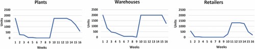
Finally, after replicating this BEM analysis to the other three main experienced scenarios (e1, e6 and e16), the amplification of the net inventory value is also similar at each SC level (see Table 6).

Regarding the managerial implications for BUF, the presented SCP model demonstrates that by combining the push and pull strategies to manage inventories, costs can be reduced (scenarios e7 and e13), even with multiple demand sources of firm orders and forecasts, as well as sourcing from suppliers in disruptive situations. Managers should consider using MRP systems with JIT production to ensure operational performance improvements in terms of the total profit for all the involved problem sizes compared to using a traditional MRP strategy (see Tables 3 and 4).

7. Conclusions

The first research objective of this paper is the design and formulation of a new tactical and operational mathematical model, LSCP 4.0 for PPC in a traditional multilevel SC context (Section 5). Then by experimenting with LSCP 4.0, which is the second research objective (Section 6), we demonstrate that using mixed MRP and JIT planning systems can serve as a proactive measure of resilience to possible demand variability disruptions in SCs. In particular, into MILP we integrate the orders from firm orders with pull demand and the forecasts with push demand in a five-level SC. Other resilient practices are also applied to select the first-level backup suppliers in a profit maximisation problem. In sustainability terms, the model incorporates costs related to carbon emissions in the first-level suppliers’ production processes. The novelty of the applied case studies, which is the third research objective (Subsection 6.2), lies in demonstrating that applying lean practices, such as JIT production, can improve the performance of a traditional footwear SC in terms of decreased inventory costs and the bullwhip effect.

7.1. Implications to theory and practice

The main results from this study are summarised as follows:

• Providing a novel multilevel model for SC planning that considers a combination of push and pull strategies for inventory control, which integrates lean, resilient and sustainable aspects. Here the computational results show that inventory costs tend to be lower when using MRP systems at higher SC levels, while JIT production systems applied at lower SC levels stabilises inventory levels and improves overall performance costs.

• The LSCP 4.0 model obtains feasible expected profit solutions for a real case study in the footwear industry with three different problem sizes based on irregular demand datasets: small, medium and large. The outcomes indicated that as problem size grows, inventory levels tend to stabilise in the MRP and JIT scenarios. Consequently, when comparing both strategies, the mixed approach is recommended for LSCP because it offers lower backorder and penalty costs for the possible need of slack for JIT production for all the problem sizes.

• The measurements of the bullwhip effect in the best mixed SC scenario under study reflect a fluctuation of orders caused by upstream demand amplification, which amounts to 18.6% at the fourth SC level (suppliers level 1). These values improve the SC’s performance compared to the theoretical foundations that present 35% in, for example, the textile industry (Towill and McCullen 1999).

7.2. Key lessons learnt

LM can be applied to a traditional five-level SC with positive effects on performance. Nevertheless, researchers and practitioners should implement combined JIT and MRP operations strategies to achieve better SC performance in terms of reducing production, inventory, backorders, transportation and environmental costs. Consequently, the knowledge acquired from this study can be used to foster the experimentation and validation of SC operations strategies at the three decision levels, i.e. strategic, tactical and operational, by mathematical programming models, which support the decision-making processes effectively in real-world problems that target other industry types.

7.3. Limitations and future research

Regarding the limitations and further research of our proposal, firstly the data about all the footwear company’s demands are limited to operational decisions. This implies that more information can be experimented with in a tactical and strategic environment. The model has also been designed with a single objective, that of profit maximisation. So the next stage can be extended to multiple objectives of the LSCP 4.0 model by, for instance, considering the social aspect of the sustainability in the objective function. Additionally, future work aims to extend experimentation to other types of SC structures, such as lean, e-procurement-based, electronic point of sales and vendor management inventory. In line with this, we encourage other researchers to apply the model presented herein to case studies from other industrial sectors by using other LM tools, for example Kanban. Moreover, future research could consider using other I4.0 technologies, such as big data analytics and trace and tracking systems, to address the problem of information exchange between supply network nodes. Future work could also incorporate decision making under uncertainty for supplier selection in the event of disruptions through robust, stochastic or fuzzy optimisation. Last but not least, other potential research would be related to approach a decentralised and collaborative SC, in which factories perform the BOMs explosion to first-level and second-level suppliers to diminish the bullwhip effect along the upstream SC. Finally, a forthcoming work aims to generate a Python code using Pyomo and Gurobi to provide our model with more flexibility and computational efficiency during operational processes through the C2NET manufacturing platform.

Acknowledgements

The research that has led to the present results has received funding from: the European Union H2020 Programme with grant agreement No. 958205 ‘Industrial Data Services for Quality Control in Smart Manufacturing (i4Q)’; the MCIN/AEI/10.13039/501100011033 and by European Union Next Genera-tionEU/PRTR with grant agreement PDC2022-133957-I00; the Regional Department of Innovation, Universities, Science and Digital Society of the Generalitat Valenciana entitled ‘Industrial Production and Logistics Optimization in Industry 4.0’ (i4OPT) (Ref. PROMETEO/2021/065); ‘Resilient, Sustainable and People-Oriented Supply Chain 5.0 Optimization Using Hybrid Intelligence’ (RESPECT) (Ref. CIGE/2021/159); and a PhD grant from the Universidad Técnica de Ambato.

Disclosure statement

No potential conflict of interest was reported by the author(s).

Data availability statement

The authors confirm that the data supporting the findings of this study are available in the article and in Appendix.

Additional information

Funding

This work was supported by Generalitat Valenciana [grant numbers: PROMETEO/2021/065 and CIGE/2021/159]; Horizon 2020 Framework Programme [grant number 958205]; the MCIN/AEI/10.13039/501100011033 and by European Union Next GenerationEU/PRTR [grant number PDC2022-133957-I00]; and Universidad Técnica de Ambato.

Notes on contributors

John Reyes

John Reyes is Aggregate Professor in the Universidad Técnica de Ambato (UTA), Ecuador. He is Master of Industrial Engineering, graduated from the University of Santiago de Chile. He has worked as an Industrial Engineer in the area of consulting for mining companies and the footwear sector, where he has been involved in logistical, operational and management processes, as well as in the area of risk analysis. He is currently pursuing a PhD programme in engineering and industrial production at the Universitat Politècnica de València (UPV), Spain. His research interests include information technologies, industrial engineering, supply chain management, operations research, lean manufacturing tools, business process management, and modelling and simulation.

Josefa Mula

Josefa Mula is Professor in the Department of Business Management of the Universitat Politècnica de València (UPV), Spain. She is a member of the Research Centre on Production Management and Engineering (CIGIP) of the UPV. Her teaching and principal research interests concern industrial engineering, production research, operations research and supply chain simulation. She is editor in chief of the International Journal of Production Management and Engineering. She regularly acts as associate editor, guest editor, member of scientific committees of international journals and conferences, and as reviewer of scientific journals. She is co-author of more than 130 articles published in international books and high-quality journals. Currently, she is principal investigator of the Valencian regional project ‘Industrial Production and Logistics Optimization in Industry 4.0 (i4OPT)’ (PROMETEO/2021/065), and the Spanish national project ‘Validation of transferable results of optimisation of zero-defect enabling production technologies for supply chain 4.0 (CADS4.0-II)’ (PDC2022-133957-I00); and UPV coordinator of the European project ‘Social and hUman ceNtered XR (SUN XR)’ (101092612).

Manuel Diaz-Madroñero

Manuel Diaz-Madroñero is Associate Professor in the Department of Business Management of the Universitat Politècnica de València (UPV), Spain. He teaches subjects related to Information Systems, Operational Research and Operations Management and Logistics. He is member of the Research Centre on Production Management and Engineering (CIGIP) of the UPV. He has participated in different research projects funded by the European Commission, the Spanish Government, the Valencian Regional Goverment and the UPV. As a result, he has published (in collaboration) more than forty articles in different indexed journals and international conferences. He is member of several scientific committees of international journals and conferences, and participates as reviewer of scientific journals. His research areas include production planning and transportation, fuzzy mathematical programming and robust optimisation, multicriteria decision making and sustainable operations management.

References

- Alavidoost, M. H., A. Jafarnejad, and H. Babazadeh. 2021. “A Novel Fuzzy Mathematical Model for an Integrated Supply Chain Planning Using Multi-Objective Evolutionary Algorithm.” Soft Computing 25: 1777–1801. https://doi.org/10.1007/s00500-020-05251-6.
- Andres, Beatriz, Raul Poler, and Raquel Sanchis. 2021. “A Data Model for Collaborative Manufacturing Environments.” Computers in Industry 126: 103398. https://doi.org/10.1016/j.compind.2021.103398.
- Becerra, P., J. Mula, and R. Sanchis. 2021. “Green Supply Chain Quantitative Models for Sustainable Inventory Management: A Review.” Journal of Cleaner Production 328: 129544. https://doi.org/10.1016/j.jclepro.2021.129544.
- Biswas, P., and B. Sarker. 2020. “Operational Planning of Supply Chains in a Production and Distribution Center with Just-in-Time Delivery.” Journal of Industrial Engineering and Management 13 (2): 332–351. https://doi.org/10.3926/JIEM.3046.
- Bortolotti, T., P. Danese, and P. Romano. 2013. “Assessing the Impact of Just-in-Time on Operational Performance at Varying Degrees of Repetitiveness.” International Journal of Production Research 51 (4): 1117–1130. https://doi.org/10.1080/00207543.2012.678403.
- Boutsioli, Zoe. 2010. “Demand Variability, Demand Uncertainty and Hospital Costs: A Selective Survey of the Empirical Literature.” Global Journal of Health Science 2 (1): 138–149. https://doi.org/10.5539/gjhs.v2n1p138.
- Brunaud, B., J. M. Laínez-Aguirre, J. M. Pinto, and I. E. Grossmann. 2019. “Inventory Policies and Safety Stock Optimization for Supply Chain Planning.” AIChE Journal 65 (1): 99–112. https://doi.org/10.1002/aic.16421.
- Cameron, Ian T, and Katalin Hangos. 2001. Process Modelling and Model Analysis. Fourth. San Diego: Academic Press.
- Cheah, Lynette, Natalia Duque Ciceri, Elsa Olivetti, Seiko Matsumura, Dai Forterre, Richard Roth, and Randolph Kirchain. 2013. “Manufacturing-Focused Emissions Reductions in Footwear Production.” Journal of Cleaner Production 44: 18–29. https://doi.org/10.1016/j.jclepro.2012.11.037.
- Chen, F., Z. Drezner, J. K. Ryan, and D. Simchi-Levi. 2000. “Quantifying the Bullwhip Effect in a Simple Supply Chain: The Impact of Forecasting, Lead Times, and Information.” Management Science 46 (3): 436–443. https://doi.org/10.1287/mnsc.46.3.436.12069.
- Chen, Z., and J. S. Shang. 2008. “Manufacturing Planning and Control Technology Versus Operational Performance: An Empirical Study of MRP and JIT in China.” International Journal of Manufacturing Technology and Management 13 (1): 4–29. https://doi.org/10.1504/IJMTM.2008.015971.
- Coronado Mondragon, Adrian E, and Andrew C Lyons. 2008. “Investigating the Implications of Extending Synchronized Sequencing in Automotive Supply Chains: The Case of Suppliers in the European Automotive Sector.” International Journal of Production Research 46 (11): 2867–2888. https://doi.org/10.1080/00207540601055466.
- Danese, P., V. Manfè, and P. Romano. 2018. “A Systematic Literature Review on Recent Lean Research: State-of-the-art and Future Directions.” International Journal of Management Reviews 20 (2): 579–605. https://doi.org/10.1111/ijmr.12156.
- Das, Kanchan. 2018. “Integrating Lean Systems in the Design of a Sustainable Supply Chain Model.” International Journal of Production Economics 198 (November 2017): 177–190. https://doi.org/10.1016/j.ijpe.2018.01.003.
- Das, Kanchan. 2019. “Integrating Lean, Green, and Resilience Criteria in a Sustainable Food Supply Chain Planning Model.” International Journal of Mathematical, Engineering and Management Sciences 4 (2): 259–275. https://doi.org/10.33889/ijmems.2019.4.2-022.
- Díaz-Madroñero, Manuel, Josefa Mula, and David Peidro. 2014. “A Review of Discrete-Time Optimization Models for Tactical Production Planning.” International Journal of Production Research 52 (17): 5171–5205. https://doi.org/10.1080/00207543.2014.899721.
- Díaz-Madroñero, Manuel, David Peidro, and Josefa Mula. 2015. “A Review of Tactical Optimization Models for Integrated Production and Transport Routing Planning Decisions.” Computers and Industrial Engineering 88: 518–535. https://doi.org/10.1016/j.cie.2015.06.010.
- Dunke, Fabian, Iris Heckmann, Stefan Nickel, and Francisco Saldanha-da-Gama. 2018. “Time Traps in Supply Chains: Is Optimal Still Good Enough?” European Journal of Operational Research 264 (3): 813–829. https://doi.org/10.1016/j.ejor.2016.07.016.
- Fahimnia, B., H. Davarzani, and A. Eshragh. 2018. “Planning of Complex Supply Chains: A Performance Comparison of Three Meta-Heuristic Algorithms.” Computers and Operations Research 89: 241–252. https://doi.org/10.1016/j.cor.2015.10.008.
- Fahimnia, B., J. Sarkis, and A. Eshragh. 2015. “A Tradeoff Model for Green Supply Chain Planning: A Leanness-versus-Greenness Analysis.” Omega-International Journal of Management Science 54: 173–190. https://doi.org/10.1016/j.omega.2015.01.014.
- Farahani, R. Z., and M. Elahipanah. 2008. “A Genetic Algorithm to Optimize the Total Cost and Service Level for Just-in-Time Distribution in a Supply Chain.” International Journal of Production Economics 111 (2): 229–243. https://doi.org/10.1016/j.ijpe.2006.11.028.
- Fransoo, J. C., and M. J. F. Wouters. 2000. “Measuring the Bullwhip Effect in the Supply Chain.” Supply Chain Management: An International Journal 5 (2): 78–89. https://doi.org/10.1108/13598540010319993.
- Ganeshan, Ram. 1999. “Managing Supply Chain Inventories: A Multiple Retailer, One Warehouse, Multiple Supplier Model.” International Journal of Production Economics 59 (1-3): 341–354. https://doi.org/10.1016/S0925-5273(98)00115-7.
- Ghahremani-Nahr, Javid, and Abdolsalam Ghaderi. 2022. “Robust-Fuzzy Optimization Approach in Design of Sustainable Lean Supply Chain Network Under Uncertainty.” Computational & Applied Mathematics 41: 255. https://doi.org/10.1007/s40314-022-01936-w.
- Gholami-Zanjani, S. M., M. S. Jabalameli, and M. S. Pishvaee. 2021. “A Resilient-Green Model for Multi-Echelon Meat Supply Chain Planning.” Computers and Industrial Engineering 152: 107018. https://doi.org/10.1016/j.cie.2020.107018.
- Govindan, K., and T. C. E. Cheng. 2018. “Advances in Stochastic Programming and Robust Optimization for Supply Chain Planning.” Computers and Operations Research 100: 262–269. https://doi.org/10.1016/j.cor.2018.07.027.
- Green, K. W., R. A. Inman, V. E. Sower, and P. J. Zelbst. 2019. “Impact of JIT, TQM and Green Supply Chain Practices on Environmental Sustainability.” Journal of Manufacturing Technology Management 30 (1): 26–47. https://doi.org/10.1108/JMTM-01-2018-0015.
- Guzman, E., B. Andres, and R. Poler. 2022. “Models and Algorithms for Production Planning, Scheduling and Sequencing Problems: A Holistic Framework and a Systematic Review.” Journal of Industrial Information Integration 27: 100287. https://doi.org/10.1016/j.jii.2021.100287.
- Hein, F., and C. Almeder. 2016. “Quantitative Insights into the Integrated Supply Vehicle Routing and Production Planning Problem.” International Journal of Production Economics 177: 66–76. https://doi.org/10.1016/j.ijpe.2016.04.014.
- Ivanov, D., and A. Dolgui. 2021. “OR-Methods for Coping with the Ripple Effect in Supply Chains During COVID-19 Pandemic: Managerial Insights and Research Implications.” International Journal of Production Economics 232: 107921. https://doi.org/10.1016/j.ijpe.2020.107921.
- Ivanov, D., A. Dolgui, and B. Sokolov. 2019. “The Impact of Digital Technology and Industry 4.0 on the Ripple Effect and Supply Chain Risk Analytics.” International Journal of Production Research 57 (3): 829–846. https://doi.org/10.1080/00207543.2018.1488086.
- Karakutuk, S Serhat, and M Arslan Ornek. 2023. “A Goal Programming Approach to Lean Production System Implementation.” Journal of the Operational Research Society 74 (1): 403–416. https://doi.org/10.1080/01605682.2022.2046518.
- Kaur, H., S. P. Singh, J. A. Garza-Reyes, and N. Mishra. 2020. “Sustainable Stochastic Production and Procurement Problem for Resilient Supply Chain.” Computers and Industrial Engineering 139: 105560. https://doi.org/10.1016/j.cie.2018.12.007.
- Lahrichi, Youssef, David Damand, and Marc Barth. 2022. “A First MILP Model for the Parameterization of Demand-Driven MRP.” Computers and Industrial Engineering 174: 108769. https://doi.org/10.1016/j.cie.2022.108769.
- Lander, E., and J. K. Liker. 2007. “The Toyota Production System and Art: Making Highly Customized and Creative Products the Toyota Way.” International Journal of Production Research 45 (16): 3681–3698. https://doi.org/10.1080/00207540701223519.
- Lee, Hau L., V. Padmanabhan, and Seungjin Whang. 1997. “Information Distortion in a Supply Chain: The Bullwhip Effect.” Management Science 43 (4): 546–558. https://doi.org/10.1287/mnsc.43.4.546.
- Lejarza, Fernando, Morgan T Kelley, and Michael Baldea. 2022. “Feedback-Based Deterministic Optimization is a Robust Approach for Supply Chain Management Under Demand Uncertainty.” Industrial and Engineering Chemistry Research 61 (33): 12153–12168. https://doi.org/10.1021/acs.iecr.2c00099.
- Llaguno, A., J. Mula, and F. Campuzano-Bolarin. 2022. “State of the Art, Conceptual Framework and Simulation Analysis of the Ripple Effect on Supply Chains.” International Journal of Production Research 60 (6): 2044–2066. https://doi.org/10.1080/00207543.2021.1877842.
- Lobo Mesquita, L., F. L. Lizarelli, S. Duarte, and P. C. Oprime. 2021. “Exploring Relationships for Integrating Lean, Environmental Sustainability and Industry 4.0.” International Journal of Lean Six Sigma 13 (4): 863–896. https://doi.org/10.1108/IJLSS-09-2020-0145.
- Malmir, Behnam, and Christopher W. Zobel. 2021. “An Applied Approach to Multi-Criteria Humanitarian Supply Chain Planning for Pandemic Response.” Journal of Humanitarian Logistics and Supply Chain Management 11 (2): 320–346. https://doi.org/10.1108/JHLSCM-08-2020-0064.
- Mehrjerdi, Y. Z., and M. Shafiee. 2021. “A Resilient and Sustainable Closed-Loop Supply Chain Using Multiple Sourcing and Information Sharing Strategies.” Journal of Cleaner Production 289: 125141. https://doi.org/10.1016/j.jclepro.2020.125141.
- Mula, J., A. C. Lyons, J. E. Hernández, and R. Poler. 2014. “An Integer Linear Programming Model to Support Customer-Driven Material Planning in Synchronised, Multi-Tier Supply Chains.” International Journal of Production Research 52 (14): 4267–4278. https://doi.org/10.1080/00207543.2013.878055.
- Mula, J., R. Poler, and J. P. Garcia. 2006. “MRP with Flexible Constraints: A Fuzzy Mathematical Programming Approach.” Fuzzy Sets and Systems 157 (1): 74–97. https://doi.org/10.1016/j.fss.2005.05.045.
- Oh, J., and B. Jeong. 2019. “Tactical Supply Planning in Smart Manufacturing Supply Chain.” Robotics and Computer-Integrated Manufacturing 55: 217–233. https://doi.org/10.1016/j.rcim.2018.04.003.
- Orlicky, J. 1975. Material Requirements Planning. London: McGraw Hill.
- Pahl, Julia, and Stefan Voß. 2014. “Integrating Deterioration and Lifetime Constraints in Production and Supply Chain Planning: A Survey.” European Journal of Operational Research 238 (3): 654–674. https://doi.org/10.1016/j.ejor.2014.01.060.
- Panwar, A., B. P. Nepal, R. Jain, and A. P. S. Rathore. 2015. “On the Adoption of Lean Manufacturing Principles in Process Industries.” Production Planning and Control 26 (7): 564–587. https://doi.org/10.1080/09537287.2014.936532.
- Pearce, A., and D. Pons. 2019. “Advancing Lean Management: The Missing Quantitative Approach.” Operations Research Perspectives 6: 100114. https://doi.org/10.1016/j.orp.2019.100114.
- Psomas, E. 2021. “Future Research Methodologies of Lean Manufacturing: A Systematic Literature Review.” International Journal of Lean Six Sigma 12 (6): 1146–1183. https://doi.org/10.1108/IJLSS-06-2020-0082.
- Rabbani, M., S. Aghamohamadi-Bosjin, and N. Manavizadeh. 2021. “Leagile Supply Chain Network Design through a Dynamic Two-Phase Optimization in View of Order Penetration Point.” RAIRO - Operations Research 55: S1369–S1394. https://doi.org/10.1051/ro/2020041.
- Reyes, John, Josefa Mula, and Manuel Díaz-Madroñero.2023a. “Optimisation Modeling for Lean, Resilient, Flexible and Sustainable Supply Chain Planning, edited by IoT and Data Science in Engineering Management. CIO 2022.. Lecture Notes on Data Engineering and Communications Technologies, Vol. 60, edited by F. P. García-Márquez, I. Segovia-Ramírez, P. J. Bernalte-Sánchez, and A. Muñoz-del-Río, 341–345. Cham: Springer. https://doi.org/10.1007/978-3-031-27915-7_60.
- Reyes, John, Josefa Mula, and Manuel Díaz-Madroñero. 2023b. “Development of a Conceptual Model for Lean Supply Chain Planning in Industry 4.0: Multidimensional Analysis for Operations Management.” Production Planning & Control 34 (12): 1209–1224. https://doi.org/10.1080/09537287.2021.1993373.
- Reyes, John, Josefa Mula, Manuel Díaz-Madroñero, and Beatriz Andrez. 2024. “Normalised Data Model for Cloud Collaborative Manufacturing: Applied to the Footwear Industry.” In CIO 2023. Lecture Notes on Data Engineering and Communications Technologies, In Press.
- Rota, K., C. Thierry, and G. Bel. 1997. “Capacity-Constrained MRP System: A Mathematical Programming Model Integrating Firm Orders, Forecasts and Suppliers.” Université Toulouse II Le Mirail.
- Roy, R. N. 2020. “Implementing Just-in-Time-Based Supply Chain for the Bulk Items in an Integrated Steel Plant.” International Journal of Intelligent Enterprise 7 (4): 405–421. https://doi.org/10.1504/ijie.2020.110762.
- Shafiee, M., Y. Zare Mehrjerdi, and M. Keshavarz. 2021. “Integrating Lean, Resilient, and Sustainable Practices in Supply Chain Network: Mathematical Modelling and the AUGMECON2 Approach.” International Journal of Systems Science: Operations and Logistics 9 (4): 451–471. https://doi.org/10.1080/23302674.2021.1921878.
- Shapiro, Jeremy F. 2004. “Challenges of Strategic Supply Chain Planning and Modeling.” Computers & Chemical Engineering 28 (6-7): 855–861. https://doi.org/10.1016/j.compchemeng.2003.09.013.
- Sugimori, Y., K. Kusunoki, F. Cho, and S. Uchikawa. 1977. “Toyota Production System and Kanban System Materialization of Just-in-Time and Respect-for-Human System.” International Journal of Production Research 15 (6): 553–564. https://doi.org/10.1080/00207547708943149.
- Tirkolaee, E. B., A. Mardani, Z. Dashtian, M. Soltani, and G.-W. Weber. 2020. “A Novel Hybrid Method Using Fuzzy Decision Making and Multi-Objective Programming for Sustainable-Reliable Supplier Selection in Two-Echelon Supply Chain Design.” Journal of Cleaner Production 250: 119517. https://doi.org/10.1016/j.jclepro.2019.119517.
- Towill, Denis R., and Peter McCullen. 1999. “The Impact of Agile Manufacturing on Supply Chain Dynamics.” The International Journal of Logistics Management 10 (1): 83–96. https://doi.org/10.1108/09574099910805879.
- Vafaeenezhad, T., R. Tavakkoli-Moghaddam, and N. Cheikhrouhou. 2019. “Multi-Objective Mathematical Modeling for Sustainable Supply Chain Management in the Paper Industry.” Computers and Industrial Engineering 135: 1092–1102. https://doi.org/10.1016/j.cie.2019.05.027.
- Vidal, Germán Herrera. 2023. “Deterministic and Stochastic İnventory Models in Production Systems: A Review of the Literature.” Process Integration and Optimization for Sustainability 7 (1-2): 29–50. https://doi.org/10.1007/s41660-022-00299-3.
- Wang, W., R. Y. K. Fung, and Y. Chai. 2004. “Approach of Just-in-Time Distribution Requirements Planning for Supply Chain Management.” International Journal of Production Economics 91 (2): 101–107. https://doi.org/10.1016/S0925-5273(03)00212-3.
- Wang, S., and B. R. Sarker. 2006. “Optimal Models for a Multi-Stage Supply Chain System Controlled by Kanban Under Just-in-Time Philosophy.” European Journal of Operational Research 172 (1): 179–200. https://doi.org/10.1016/j.ejor.2004.10.001.
- Williams, H. P. 2013. Model Building in Mathematical Programming. 5th ed. Chichester, West Sussex: John Wiley & Sons.
- Winston, Wayne L. 2004. Operations Research: Applications and Algorithms. 4th ed. Belmont, CA: Thomson Learning.
- Yang, J., H. Xie, G. Yu, and M. Liu. 2021. “Achieving a Just–in–Time Supply Chain: The Role of Supply Chain Intelligence.” International Journal of Production Economics 231: 107878. https://doi.org/10.1016/j.ijpe.2020.107878.
- Zamanian, M. R., E. Sadeh, Z. Amini Sabegh, and R. Ehtesham Rasi. 2020. “A Multi-Objective Optimization Model for the Resilience and Sustainable Supply Chain: A Case Study.” International Journal of Supply and Operations Management 7 (1): 51–75. https://doi.org/10.22034/IJSOM.2020.1.4.
- Zekhnini, K., A. Cherrafi, I. Bouhaddou, A Chaouni Benabdellah, and S. Bag. 2021. “A Model Integrating Lean and Green Practices for Viable, Sustainable, and Digital Supply Chain Performance.” International Journal of Production Research 60 (21): 6529–6555. https://doi.org/10.1080/00207543.2021.1994164.